ACTIVA: realistic single-cell RNA-seq generation with automatic cell-type identification using introspective variational autoencoders

Abstract

Motivation

Single-cell RNA sequencing (scRNAseq) technologies allow for measurements of gene expression at a single-cell resolution. This provides researchers with a tremendous advantage for detecting heterogeneity, delineating cellular maps or identifying rare subpopulations. However, a critical complication remains: the low number of single-cell observations due to limitations by rarity of subpopulation, tissue degradation or cost. This absence of sufficient data may cause inaccuracy or irreproducibility of downstream analysis. In this work, we present Automated Cell-Type-informed Introspective Variational Autoencoder (ACTIVA): a novel framework for generating realistic synthetic data using a single-stream adversarial variational autoencoder conditioned with cell-type information. Within a single framework, ACTIVA can enlarge existing datasets and generate specific subpopulations on demand, as opposed to two separate models [such as single-cell GAN (scGAN) and conditional scGAN (cscGAN)]. Data generation and augmentation with ACTIVA can enhance scRNAseq pipelines and analysis, such as benchmarking new algorithms, studying the accuracy of classifiers and detecting marker genes. ACTIVA will facilitate analysis of smaller datasets, potentially reducing the number of patients and animals necessary in initial studies.

Results

We train and evaluate models on multiple public scRNAseq datasets. In comparison to GAN-based models (scGAN and cscGAN), we demonstrate that ACTIVA generates cells that are more realistic and harder for classifiers to identify as synthetic which also have better pair-wise correlation between genes. Data augmentation with ACTIVA significantly improves classification of rare subtypes (more than 45% improvement compared with not augmenting and 4% better than cscGAN) all while reducing run-time by an order of magnitude in comparison to both models.

Availability and implementation

The codes and datasets are hosted on Zenodo (https://doi.org/10.5281/zenodo.5879639). Tutorials are available at https://github.com/SindiLab/ACTIVA.

Supplementary information

Supplementary data are available at Bioinformatics online.

1 Introduction

Traditional sequencing methods are limited to measuring the average signal in a group of cells, which potentially mask heterogeneity and rare populations (Tang et al., 2019). Single-cell RNA sequencing (scRNAseq) technologies allow for the amplification and extraction of small RNA quantities, which enable sequencing at a single-cell level (Tang et al., 2009). The single-cell resolution thus enhances our understanding of complex biological systems. For example, in the immune system scRNAseq has been used to discover new immune cell populations, targets and relationships, which have been used to propose new treatments (Tang et al., 2019).

While the number of tools for analyzing scRNAseq data increases, one limiting factor remains: low number of cells, potentially related to financial, ethical, or patient availability (Marouf et al., 2020). Large well-funded projects have generated the Human Cell Atlas (Regev et al., 2017) and the Mouse Cell Atlas (Han et al., 2018) which characterized cell populations in organs and tissues in their respective species. Although a tremendous amount of scRNAseq data is available from such projects, they are limited to a broad overview of the cell populations in these tissues and organs. The Atlases overlook sub-populations of cells which tend to be smaller, rarer and important players in normal and dysregulated states. As Button et al. (2013) note, small numbers of observations reduce the reproducibility and robustness of experimental results. This is especially important for benchmarking new tools for scRNAseq data, as the number of features (genes) in each cell often exceeds the number of samples.

Given limitations on scRNAseq data availability and the importance of adequate sample sizes, in silico data generation and augmentation offers a fast, reliable and cheap solution. Synthetic data augmentation is a standard practice in fields of machine learning such as text and image classification (Shorten and Khoshgoftaar, 2019). Traditional data augmentation techniques, geometric transformations or noise injection, are being replaced by more recently developed generative models, variational autoencoder (VAE) (Kingma and Welling, 2013) and Generative Adversarial Networks (GANs) (Goodfellow et al., 2014), for augmenting complex biological datasets. However, GANs and VAEs remain less explored for data augmentation in genomics and transcriptomics. We provide a brief overview of GANs and VAEs in Section 2 and in Supplementary Material.

There are many statistical frameworks for generating in-silico scRNAseq data (Assefa et al., 2020; Benidt and Nettleton, 2015; Frazee et al., 2015; Gerard, 2020; Zhang et al., 2019), but recently Marouf et al. (2020) introduced the first deep generative models (GAN-based) for scRNAseq data generation and augmentation [called single-cell GAN (scGAN) and conditional scGAN (cscGAN)], and demonstrated that they outperform other state-of-the-art models. While scGAN augments the entire population by creating ‘holistic’ cells, cscGAN is conditioned to generate cells from specific subpopulations.

In this work, we extend and generalize their approach using an introspective VAE for data augmentation. The motivation and application of our generative model is closely related to Marouf et al.’s, with a focus on improving training time, stability and generation quality using only one framework. We compare our proposed model, Automated Cell-Type-informed Introspective Variational Autoencoder (ACTIVA), with scGAN and cscGAN and show how it can be leveraged to augment rare populations, improving classification and downstream analysis. In contrast to these previously published GANs, our novel cell-type conditioned introspective VAE model allows us to generate either ‘holistic’ or specific cellular subpopulations in a single framework.

In Section 2, we provide an overview of GANs (both generally and in the context of scRNAseq data) and VAEs. In Section 3, we detail ACTIVA, our proposed conditional introspective VAE. In Section 4, we describe our training data and associated processing steps. In Section 5, we compare ACTIVA with competing methods—scGAN and cscGAN. We demonstrate that augmenting rare cell populations with ACTIVA improves classification over GANs while providing a more computationally tractable framework, mirroring both scGAN and cscGAN, in a single model. In comparison with scGAN and cscGAN, ACTIVA generates cells that are harder for classifiers to identify as synthetic [i.e. having Areas Under the Curve (AUC) closer to 0.5], with better pair-wise correlation between genes. ACTIVA generated cells allow for improved classification of rare subtypes (more than 4% improvement over cscGAN) all while reducing run-time by an order of magnitude in comparison to both models. Finally, in Section 6, we review our approach, findings and limitations.

2 Background

2.1 Generative adversarial networks

GANs (Goodfellow et al., 2014) are capable of generating realistic synthetic data, and have been successfully applied to a wide range of machine learning tasks (Dziugaite et al., 2015) and bioinformatics (Liu et al., 2019). GANs consist of a generator network (G) and a discriminator network (D) that train adversarially, which enables them to produce high-quality fake samples. During training, D learns the difference between real and synthetic samples, while G produces fake data to ‘fool’ D. More specifically, G produces a distribution of generated samples P_g, given an input $z\sim P_z$, with P_z being a random noise distribution. The objective of GANs is to learn P_g, ideally finding a close approximation to the real data distribution P_r, so that $P_g\approx P_r$. To learn the approximation to P_g, GANs play a ‘min-max game’ of ${\min }_G{\max }_D{\mathbb{E}}_{x\sim P_r}\hspace{0.17em}\text{log}[D(x)]+{\mathbb{E}}_{z\sim P_z}\hspace{0.17em}\text{log}[1-D(G(z))],$ where both players (G and D) attempt to maximize their own payoff. This adversarial training is critical in GANs’ ability to generate realistic samples. Compared with other generative models, GANs’ main advantages are (i) the ability to produce any type of probability density, (ii) no prior assumptions for training the generator network, and (iii) no restrictions on the size of the latent space.

Despite these advantages, GANs are notoriously hard to train since it is highly non-trivial for G and D to achieve Nash equilibrium (Wang et al., 2019). Another disadvantage of GANs are vanishing gradients where an optimal D cannot provide enough information for G to learn and make progress, as shown by Arjovsky and Bottou (2017). Another issue with GANs is ‘mode collapse’, that is, when G has learned to map several noise vectors z to the same output that D classifies as real data. In this scenario, G is over-optimized, and the generated samples lack diversity. Although some variations of GANs have been proposed to alleviate vanishing gradients and mode collapse [e.g. Wasserstein-GANs (WGANs) (Arjovsky et al., 2017) and Unrolled-GANs (Metz et al., 2016)], the convergence of GANs still remains a major problem.

2.2 Single-cell GANs

scGAN and cscGAN are the state-of-the-art deep learning models for generating and augmenting scRNAseq data. Marouf et al. (2020) train scGAN to generate single-cell data from all populations and cscGAN to produce cluster-specific samples, with the underlying model in both being a WGAN. For scGAN, the objective is to minimize Wasserstein distance between real cells distribution, P_r , and generated data, P_g:

$$W(P_r,P_g)=\underset{\gamma \in \Pi (P_r,P_g)}{\inf }{\mathbb{E}}_{(\mathbf{x},\mathbf{y})\sim \gamma }\left|\right|\mathbf{x}-\mathbf{y}\left|\right|,$$ (1)

where x and y denote random variables, $\Pi (P_r,P_g)$ is the set of all joint probability distributions $\gamma (\mathbf{x},\mathbf{y})$ with marginals P_r and P_g. Intuitively, Wasserstein distance is the cost of optimally transporting ‘masses’ from x to y such that P_r is transformed to P_g (Arjovsky et al., 2017). However, since the infimum in Equation (1) is highly intractable, Arjovsky et al. (2017) use Kantorovich–Rubinstein duality to find an equivalent formulation of Wasserstein distance with better properties:

$$W(P_r,P_g)=\underset{\left|\right|f|{|}_L\le 1}{\sup }{\mathbb{E}}_{\mathbf{x}\sim P_r}\mathbf{f}(\mathbf{x})-{\mathbb{E}}_{\mathbf{x}\sim P_g}\mathbf{f}(\mathbf{x}),$$

where the set of 1-Lipschitz functions is denoted by $\left|\right|f|{|}_L\le 1$, with the solution being a universal approximator (potentially a fully connected neural network) to approximate f. This function is approximated by D, which we denote as f_d. Similarly, f_g denotes the function approximated by the generator. Using these notations, we arrive at the adversarial objective function of WGANs (used in scGAN):

$$\underset{f_g}{\min }\underset{\left|\right|f_d|{|}_L\le 1}{\max }{\mathbb{E}}_{\mathbf{x}\sim P_r}{\mathbf{f}}_{\mathbf{d}}(\mathbf{x})-{\mathbb{E}}_{\mathbf{x}\sim f_g(P_n)}{\mathbf{f}}_{\mathbf{d}}(\mathbf{x}),$$

where P_n denotes a multivariate noise distribution.

Although WGANs can alleviate the vanishing gradient issue, the majority of GANs’ training instabilities can still occur, making WGANs less flexible and transferable between different datasets or domain-specific tasks. CscGAN uses a projection-based conditioning (Miyato and Koyama, 2018) which adds an inner product of class labels (cell types) at the discriminator’s output. Based on instruction given by the authors in the implementation, scGAN and cscGAN must be trained separately; however, our model learns to generate specific cell populations (cell-types) or collective cell clusters with one training.

2.3 Variational autoencoders

VAEs (Kingma and Welling, 2013) are generative models that jointly learn deep latent-variable and inference models. Specifically, VAEs are autoencoders that use variational inference to reconstruct the original data, having the ability to generate new data that is ‘similar’ to those already in a dataset x. VAEs assume that observed data and latent representation are jointly distributed as $P_{\theta }(x,z)=P_{\theta }(x|z)P(z)$. In deep learning, the log-likelihood $P_{\theta }(x|z)$ is modeled through non-linear transformations, thus making the posterior probability distribution, $P_{\theta }(z|x)=\frac{P_{\theta }(x|z)P_{\theta }(z)}{P_{\theta }(x)}$, intractable. Due to the intractability of maximizing the expected log-likelihood of observed data over θ, ${\mathbb{E}}_{p(x)}\left[\text{log}\hspace{0.17em}\int P_{\theta }(x,z)dz\right]$, the goal is to instead maximize the evidence lower bound (ELBO):

$$\underset{\text{ELBO}(\theta ,\gamma )}{\underbrace{{\mathbb{E}}_{Q_{\gamma (x)}(z)}\left[\text{log}\hspace{0.17em}\left(\frac{P_{\theta }(x|z)P(z)}{Q_{\gamma (x)}(z)}\right)\right]}}\le \text{log}\hspace{0.17em}{P}_{\theta }(x),$$

where $Q_{\gamma (x)}(z)$ is an auxiliary variational distribution (with parameters $\gamma (x)$) that tries to approximate the true posterior $P_{\theta }(z|x)$.

The main issue with VAEs arises when the training procedure falls into the trivial local optimum of the ELBO objective; that is, when the variational posterior and the true posterior closely match the prior (or collapse to the prior). This phenomenon often causes issues with data generation since the generative model ignores a subset of latent variables that may have meaningful latent features for inputs (He et al., 2019). In our experiments, we did not encounter posterior collapse. However, in our package, we provide an option for modifying objective function weights adaptively using SoftAdapt (Heydari et al., 2019). VAEs have also been criticized for generating samples that adhere to an average of the data points, as opposed to sharp samples that GANs produce because of adversarial training. This issue has often been addressed by defining an adversarial training between the encoder and the decoder, as done in introspective VAEs (IntroVAEs) (Huang et al., 2018) which we use in our framework [Here, we follow Huang et al. (2018) and categorize IntroVAEs as a type of VAE.]. IntroVAEs have been used mostly in computer vision, which have performed comparably to their GAN counterparts, in applications such as synthetic image generation (Huang et al., 2018) and single-image super-resolution (Heydari and Mehmood, 2020). We describe the formulations of IntroVAEs in Section 3.

VAEs’ natural ability to produce both a generative and an inference model presents them as an ideal candidate for generation and augmentation of omics data. In this work, we demonstrate the ability of our deep VAE-based model for producing realistic in silico scRNAseq data. Our model, ACTIVA, performs comparably to the state-of-the-art GAN models, scGAN and cscGAN, and trains significantly faster and maintains stability. Moreover, ACTIVA learns to generate specific cell-types and holistic population data in one training (unlike scGAN and cscGAN that train separately). On the same datasets and in the same environment, our model trains at least six times faster than scGAN. Moreover, ACTIVA can produce 100K samples in less than 2 s on a single NVIDIA Tesla V100, and 87 s on a common research laptop. ACTIVA provides researchers with a fast, flexible and reliable deep learning model for augmenting and enlarging existing datasets, improving downstream analyses robustness and reproducibility.

3 Methods and approach

Our proposed model, ACTIVA, consists of three main networks, with a self-evaluating VAE as its core and a cell-type classifier as its conditioner. In this section, we formulate the objective functions of our model and describe the training procedure.

3.1 Encoder network

The ACTIVA encoder network, Enc, serves two purposes: (i) mapping (encoding) scRNAseq data into an approximate posterior to match the assumed prior, and (ii) acting as a discriminator, judging the quality of the generated samples against training data. Therefore, Enc’s objective function is designed to train as an adversary of the generator network, resulting in realistic data generation. To approximate the prior distribution, KL divergence is used as a regularization term (denoted as L_REG) which regularizes the encoder by forcing the approximate posterior, $Q_{\varphi }(z|x)$, to match the prior, P(z) (following notation from Section 1). We assume a center isotropic multivariate Gaussian prior, since it can be reparameterized in a differentiable way into arbitrary multivariate Gaussian random variables, thus simplifying the inference process (Lopez et al., 2018). Although $P_{\theta }(x|z)$ can be parameterized in many ways, we choose an isotropic multivariate Gaussian for simplicity. However, choosing a scRNAseq-specific counts distribution as the conditional likelihood (e.g. zero-inflated binomials) may lead to some improvements in the generation process (Lopez et al., 2018).

The posterior probability is $Q_{\varphi }(z|x)=\mathcal{N}(z;\mu ,{\sigma }^2)$, where μ and σ are the mean and standard deviation, respectively, computed from the outputs of Enc. As in traditional VAEs, z is sampled from $\mathcal{N}(0,I)$ which will be used as an input to the generator network (decoder in VAEs). Due to the stochasticity of z, gradient-based backpropagation becomes difficult, but using the reparameterization trick in Kingma and Welling (2013) makes this operation tractable. That is, define $z=\mu +\sigma \odot ϵ$ with $ϵ\sim \mathcal{N}(0,I)$ which passes the stochasticity of z onto ϵ. Now given N cells and a latent vector in a D-dimensional space (i.e. $z\in {\mathbb{R}}^D$), we can compute the KL regularization:

$$L_{\mathit{REG}}=\frac{1}{2}\sum _{i=1}^N\sum _{j=1}^D\left(1+\text{log}({\sigma }_{ij}^2)+{\mu }_{ij}^2-{\sigma }_{ij}^2\right).$$ (2)

Similar to traditional VAEs, the encoder network aims at minimizing the difference between reconstructed and training cells (real data). We denote the expected negative reconstruction error as L_AE, defined as:

$$L_{AE}={\mathbb{E}}_{Q(z|x)}\left[\text{log}\hspace{0.17em}{P}_{\theta }(x|z)\right].$$ (3)

Following Huang et al. (2018), we choose the reconstruction loss L_AE to be the mean squared error between the training cells and reconstructed cells (more details in Supplementary Material SA.3).

As the last part of the network, we introduce a cell-type loss component that encourages x_r to have the same cell type as x. That is, given a classifying network C, we want to ensure that the identified type of reconstructed sample $C(x_r)=t_r$ is the same as real cell C(x) = t; we denote this as L_CT shown in Equation (6). The explicit formulation and the classifying network are described in Section 3.3. During the development of ACTIVA, Zheng et al. (2020) introduced a similar conditioning of IntroVAE framework for image synthesis, which provided significant improvements in generating new images. Given our model’s objectives, the loss function for Enc, ${\mathcal{L}}_{\mathit{Enc}}$, must encode training data and self-evaluate newly generated cells from the generator network Gen:

$$\begin{array}{c}{\mathcal{L}}_{\mathit{Enc}}=L_{\mathit{REG}}(z)+{\alpha }_1\sum _{s=r,g}{\left[m-L_{\mathit{REG}}(z_s)\right]}^{+}\hfill \\ +{\alpha }_2\left(L_{AE}(x,x_r)+L_{CT}(t,t_r)\right),\hfill \end{array}$$ (4)

where subscripts r and g denote reconstructed and generated cells from Gen, respectively. Note that, reconstructed cells x_r correspond directly to training data x, but generated cells x_g are newly produced cells. In Equation (4), ${[·]}^{+}=\max (0,·)$, and $m\in {\mathbb{R}}^{+}$ determines our network’s adversarial training, as described in Section 3.4.

3.2 Generator network

Generator network, Gen, aims at learning two tasks. First, Gen must learn a mapping of encoded training data, $z\in {\mathbb{R}}^D$, from the posterior, $Q_{\varphi }(z|x)$, back to the original feature space, ${\mathbb{R}}^M$. In the ideal mapping, reconstructed samples x_r would match training data x perfectly. To encourage learning of this objective, we minimize the mean squared error between x and x_r, as shown in Equation (3), and force cell-types of reconstructed samples to match with original cells, as shown in Equation (6). The second task of Gen is to generate realistic new samples from a random noise vector $z_n\in {\mathbb{R}}^D\sim P(z)$ (sampled from the prior P(z)) that ‘fool’ the encoder network Enc. That is, after producing new synthetic samples x_g, we calculate $\mathit{Enc}(x_g)=z_g$ to judge the quality of generated cells. Given these two objectives, the generator’s objective function is defined as

$${\mathcal{L}}_{\mathit{Gen}}={\alpha }_1\sum _{s=r,g}{L}_{\mathit{REG}}\left(\mathit{Enc}(x_s)\right)+{\alpha }_2(L_{AE}(x,x_r)+L_{CT}(t,t_r)).$$ (5)

3.3 Automated cell-type conditioning

Minimizing L_AE alone does not enforce our model to generate more cells from the rare populations, and for this reason, we introduce a cell-type matching objective. The goal of this objective is to encourage the generator to generate cells that are classified as the same type as the input data. More explicitly, the loss component L_CT will penalize the network if reconstructed cell-types are different from the training data. Given a trained classifier $C(·)$, we can express this objective as

$$L_{CT}=\frac{1}{2}\sum _{i=1}^N{\Vert t-t_r\Vert }_F^2=\frac{1}{2}\sum _{i=1}^N{\Vert C(x)-C(x_r)\Vert }_F^2.$$ (6)

For ACTIVA’s conditioning, we use an automated cell-type identification introduced by Ma and Pellegrini (2020). This network, called ACTINN, uses all genes to capture features, and focuses on the signals associated with cell variance. We chose ACTINN because of its accurate classification and efficiency in training compared to other existing models (Abdelaal et al., 2019); we provide an overview of ACTINN in Supplementary Material SH.1. Our model is also flexible to use any classifier as a conditioner, as long as an explicit loss could be computed between the predicted labels and the true labels (This is true for most classifiers.). With ACTINN as the classifier, t and t_r are logits (output layer) for x and x_r , respectively. Our implementation of ACTINN is available as a stand-alone package at https://github.com/SindiLab/ACTINN-PyTorch.

3.4 Adversarial training

The generator produces two types of synthetic cells: reconstructed cells x_r from x and newly generated cells x_g from a noise vector. While both the Enc and Gen attempt to minimize L_AE and L_CT, the encoder tries to minimize $L_{\mathit{REG}}(z)$ and maximize $L_{\mathit{REG}}(z_{r,g})$ to be greater than or equal to m. However, the generator tries to minimize $L_{\mathit{REG}}(z_{r,g})$ to minimize its objective function. This is the min-max game played by Enc and Gen. Note that, choosing m is an important step for the network’s adversarial training; we describe the strategies for the choice of m in Supplementary Material SG.

4 Datasets and preprocessing

We use the pipeline provided by Marouf et al. (2020) to pre-process the data. First, we removed genes that were expressed in less than 3 cells and cells that expressed less than 10 genes. Next, cells were normalized by total unique molecular identifiers (UMI) counts and scaled to 20 000 reads per cell. Then, we selected a ‘test set’ (approximately 10% of each dataset). Testing samples were randomly chosen considering cell ratios in each cluster (‘balanced split’). Links to raw and pre-processed datasets are available via the link provided in abstract. We describe the post-processing steps in Supplementary Material SB. Similar to Marouf et al. (2020), we use the following datasets:

68K PBMC: To compare our results with the current state-of-the-art deep learning model, scGAN/cscGAN, we trained and evaluated our model on a dataset containing 68 579 peripheral blood mononuclear cells (PBMCs) from a healthy donor (68K PBMC) (Zheng et al., 2017). 68K PBMC is an ideal dataset for evaluating generative models due to the distinct cell populations, data complexity and size (Marouf et al., 2020). After pre-processing, the data contained 17 789 genes. We then performed a balanced split on this data, which resulted in 6991 testing and 61 588 training cells.

Brain Small: This dataset contains 20,000 random samples (out of approximately 1.3 million cells) from the cortex, hippocampus and the subventricular zone of two embryonic day 18 mice. Compared to 68K PBMC, this dataset has fewer cells, and it varies in complexity and organism. After pre-processing, the data contained 17 970 genes, which we then balanced split to 1997 test cells and 18 003 training cells.

NeuroCOVID: This dataset (Heming et al., 2021) contains scRNAseq data of immune cells from the cerebrospinal fluid (CSF) of Neuro-COVID patients and patients with non-inflammatory and autoimmune neurological diseases or with viral encephalitis. Our pre-processing resulted in data of dimensions 85 414 cells × 22 824 genes, which we split to testing and training subsets as mentioned above.

5 Results

Assessing generative model quality is notoriously difficult and still remains an open research area (Lucic et al., 2018; Theis et al., 2016). Here, we apply some qualitative and quantitative metrics for evaluating synthetic scRNAseq, as used in Marouf et al. (2020). For qualitative metrics, we compare the manifold of generated and real cells using UMAP. For quantitative metrics, we train a classifier to distinguish between real and synthetic cells. To study ACTIVA’s performance, we compare our results to Marouf et al. alone since their models outperform other state-of-the-art generative models such as Splatter (Zappia et al., 2017) and SUGAR (Lindenbaum et al., 2018). Training and inference time comparisons are shown in Supplementary Material. As we show, ACTIVA generates cells that better resemble the real data, and it outperforms competing methods on improving classification of rare cell populations with data augmentation. ACTIVA is one model that can be served as an alternative to both scGAN and cscGAN, and it trains much faster than both GAN-based models (and it only needs one training).

5.1 ACTIVA trains faster than GAN-based models

To measure the efficiency of ACTIVA in comparison to the state-of-the-art GAN-based models (scGAN and cscGAN), we trained all three models in the exact same computational environment on a single GPU for each dataset (we describe the hardware used in Supplementary Material SC). Note that since scGAN and cscGAN train separately, we repeated this process five times to account for any variability, and then computed the average training time and standard deviation. As shown in Table 1, ACTIVA trains orders of magnitude faster for both datasets (approximately 17 times faster on Brain Small and 6 times faster on 68K PBMC and NeuroCOVID) and only needs one training to produce cells from all populations (scGAN’s aim) and specific cell populations (cscGAN’s purpose) (Fig. 1).

Table 1.

Average training time with sample SD (in seconds), of five iterations for the generative models

	Brain small			68K PBMC
	ACTIVA	scGAN	cscGAN	ACTIVA	scGAN	cscGAN
Average	$8074.91\pm 135.9$ ($\approx$ 2.2 h)	142 238.10 ± 705.18 ($\approx$ 39.5 h)	145 855.98 ± 335.71 ($\approx$ 40.5 h)	26 025.95 ± 127.68 ($\approx$ 7.2 h)	164 839.14 ± 503.73 ($\approx$ 45.7 h)	176 014.49 ± 192.82 ($\approx$ 48.9 h)

Note: ACTIVA (which has the capabilities of scGAN and cscGAN combined) trains much faster than both scGAN and cscGAN. Individual run-times for each iteration are provided in Supplementary Material SD.

Fig. 1.

Overview of our deep generative model, ACTIVA and its training flow. Our model consists of three networks: (i) an encoder that also acts as a discriminator (denoted by Enc), (ii) a decoder which is used as the generative network for producing new synthetic data (denoted by Gen), and (iii) an automated cell-type classification network [denoted by ACTINN as in Ma and Pellegrini (2020)]. ACTIVA is a single-stream adversarial (Introspective) Conditional VAE without the need for a training schedule (unlike most GANs). Due to this, our model has the training stability and efficiency of VAEs while producing realistic samples comparable to GANs. We describe each component of our model and the objective functions in Section 3.

5.2 ACTIVA generates realistic cells

To qualitatively evaluate the generated cells, we analyzed the 2D UMAP representation of the test set (real data) and in silico generated cells (same size as the test set). We found that the distribution and clusters match closely between ACTIVA generated cells and real cells (Fig. 3A and B and Supplementary Fig. S13). We also analyzed t-SNE embeddings of the real cells and synthetic cells generated by ACTIVA, which showed similar results. These qualitative assessments demonstrated that ACTIVA learns the underlying manifold of real data, the main goal of generative models. A key feature of ACTIVA is the cell-type conditioning which encourages the network to produce cells from all clusters. This means that generating cells with ACTIVA results in gaining cells within clusters rather than losing clusters. Due to this design choice, ACTIVA can generate more cells from the rare populations than scGAN, as shown in Figure 3A and B. ACTIVA’s flexible framework allows for adjusting the strength of the cell-type conditioning (which is a parameter in our model) for the cases where the exact data representation is more desirable.

Fig. 3.

ACTIVA generates high-quality cells that resemble both the cluster and gene expressions present in the training data. Top row: UMAP plot of ACTIVA generated cells compared with test set and scGAN generated cells, colored by clusters for 68K PBMC (A) and Brain Small (B). Bottom row: same UMAP plots as top row, colored by selected marker gene expressions. (C) corresponds the log expression for CD79A marker gene (for 68K PBMC) and (D) illustrates the same for Hmgb2 (for Brain Small). ACTIVA’s cell-type conditioning encourages to generate more cells per cluster rather than lose clusters, meaning that ACTIVA will generate more cells from the rare populations (e.g. cluster 7 of PBMC and cluster 6 of Brain Small).

Next, we quantitatively assessed the quality of the generated cells by training a random forest (RF) classifier [same as in Marouf et al. (2020)] to distinguish between real and generated cells. The goal here is to determine how ‘realistic’ ACTIVA generated cells are compared with real cells. Ideally, the classifier will not differentiate between the synthetic and real cells, thus resulting in a receiver operating characteristic (ROC) curve that is the same as randomly guessing (0.5 AUC). The RF classifier consists of 1000 trees with the Gini impurity criterion and the square root of the number of genes as the maximum number of features used. Maximum depth is set to either all leaves containing less than two samples or until all leaves are pure. We generated cells using ACTIVA and scGAN and performed a fivefold cross-validation on synthetic and real cells (test). ACTIVA performs better than scGAN with AUC scores closer to 0.5 for both datasets (Fig. 2). For Brain Small test set, the mean ACTIVA AUC is 0.62 ± 0.02 compared with scGAN’s 0.74 ± 0.01. For 68K PBMC, the mean AUC is 0.68 ± 0.01 for ACTIVA and 0.73 ± 0.01 for scGAN.

Fig. 2.

Classifying synthetic data (ACTIVA and scGAN) from real data (test set) for Brain Small (left plot) and 68K PBMC (right plot). The metrics are reported using a random forest classifier (detailed in Section 5.2) with fivefold cross-validation (marked by pastel colors in each plot). An area under the curve (AUC) of 0.5 (chance) is the ideal scenario (red dash line), and an AUC closer to this value is better.

5.3 ACTIVA generates similar gene expression profiles

To generate cells that represent all clusters, the marker gene distribution in the generated data should roughly match the gene distribution in real cells. We used UMAP representations of ACTIVA, scGAN and the test set, and colored them based on the expression levels of marker genes. Figure 3C and D shows examples of log-gene expression for marker genes from each datasets (additional examples in Supplementary Material SJ). In our qualitative assessment, ACTIVA generated cells following the real gene expression closely. For a quantitative assessment, we calculated the Pearson correlation of top five differentially expressed genes from each cluster for both ACTIVA generated cells and real data. As shown in Figure 4, the pairwise correlation of genes from the ACTIVA generated cells closely match those from the real data for both datasets. To quantify the overall gene–gene correlation for synthetic data, we define the following metric: given a correlation matrix of generated samples, G and a correlation matrix of the real data (test set), R, we compute the 1-norm of the difference in correlations to measure the discrepancy between the correlations.

$$CD(G,R)=\underset{1\le j\le n}{\max }\sum _{i=1}^n|G_{i,j}-R_{i,j}|.$$ (7)

Fig. 4.

Correlation of top five differentially expressed genes in each cluster for 68K PBMC (A) and Brain Small (B). Lower triangular of matrices indicate correlation of generated data, and upper triangular show correlation of real data (same in both plots in panels A and B). For 68K PBMC (A), we investigated pairwise correlation for a total of 55 genes and for Brain Small (B), we calculated the Pearson correlation for 40 genes. In the ideal case, the correlation plots should be symmetric, and the Correlation Discrepancy (CD), defined in Equation (7), should be zero. The gene correlations in ACTIVA match the real data more closely than scGAN, as shown in the figures and the CD score computed; ACTIVA has a CD score of 1.5816 and 4.6852 for 68K PBMC and Brain Small, respectively, compared with scGAN’s 2.2037 and 5.5937.

We refer to this metric as Correlation Discrepancy (CD) for simplicity. (In the ideal case, $CD(G,R)=0$, therefore values closer to zero indicate better performance.) Our calculations show that for 68K PBMC, ACTIVA has a CD score of 1.5816, as opposed to scGAN’s 2.2037, and for Brain Small ACTIVA outperforms scGAN with a CD score of 4.6852 compared with 5.5937. These values further quantify that generated cells from ACTIVA better preserve the gene–gene correlation present in the real data.

In addition, we plotted marker gene distribution in all cells against real cells. Supplementary Figure S12 illustrates the distribution of five marker genes from cluster 1 (LTB, LDHB, RPL11, RPL32, RPL13) and cluster 2 (CCL5, NKG7, GZMA, CST7, CTSW). We also investigated known marker genes for specific cell populations, such as for B-cells in PBMC data, finding that ACTIVA generated cells expressed these markers (CD79A, CD19 and MS4A1) in the appropriate clusters (Fig. 3C and other figures not shown here) similar to real data. Following Marouf et al., we calculated the maximum mean discrepancy (MMD) between the real data distribution and the generated ones using ACTIVA and scGAN. Simply stated, MMD is a distance metric based on embedding probabilities in a reproducing kernel Hilbert space (Gretton et al., 2012), and since MMD is a distance metric, a lower value of MMD between two distributions indicates the distribution are closer to one another. For consistency, we chose the same kernels as Marouf et al. and calculated MMD on the first 50 principal components. As shown in Table 2, ACTIVA had a lower MMD score than scGAN, demonstrating an improvement in the quality of the generated cells compared to scGAN.

Table 2.

MMD values for ACTIVA, scGAN and positive control (training set) compared with the test set

	Brain small			68K PBMC
	Training set	ACTIVA	scGAN	Training set	ACTIVA	scGAN
MMD	0.0619	0.7715	0.9686	0.0539	0.7952	0.9047

Note: ACTIVA outperforms the scGAN for both datasets, since it has a lower MMD score.

Based on qualitative and quantitative evaluations of our model, we conclude that ACTIVA has learned the underlying marker gene distribution of real data, as desired. However, we suspect that assuming a different prior in model formulation (e.g. Zero-Inflated Negative Binomial) could further improve our model’s learning of real data.

5.4 ACTIVA generates specific cell-types on demand

Since we minimize a cell-type identification loss in the training objective, ACTIVA is encouraged to produce cells that are classified correctly. Therefore, the accuracy of the generated cell-types depends on the classifier selected. In Supplementary Tables S6 and S7, we show that ACTIVA’s classifier accurately distinguishes rare cell-types, achieving an F1 score of 0.89 when trained with only 1% sub-population in the training cells. ACTIVA generates specific cell-types from the manifold it has learned, which then filters through the identifier network to produce specific sub-populations. To quantify the quality of the generated samples, we trained an RF classifier (as in Section 5.2) to distinguish between generated and real sub-populations in the data. Figure 5 illustrates ACTIVA’s performance against cscGAN for the Brain Small dataset, with ACTIVA achieving better AUC scores. Similar results were obtained for 68K PBMC sub-populations, although the AUC gap between cscGAN and ACTIVA were narrower.

Fig. 5.

RF classifier distinguishes two real sub-populations from synthetic data for Brain Small. ACTIVA outperforms cscGAN in producing realistic samples on this dataset, since the ROC curve is closer to chance (red dashed line).

5.5 ACTIVA improves classification of rare cells

A main goal of designing generative models is to augment sparse datasets with additional data that can improve downstream analyses. Given the performance of our model and conditioner, we hypothesized that classifying rare cells in a dataset can be improved through augmentation with ACTIVA, i.e. using synthetic rare cells alongside real data. We next directly compared against cscGAN to demonstrate the feasibility of augmenting rare population to improve classification. We utilized the data-augmentation experiment presented by Marouf et al. (2020). That is, we chose the cells in cluster 2 of 68K PBMC, and downsampled those cells to 10%, 5%, 1% and 0.5% of the actual cluster size, while keeping the populations fixed. The workflow of the downsampling and exact sizes is shown in Supplementary Figure S8. We then trained ACTIVA on the downsampled subsets, and generated 1500 synthetic cluster 2 cells to augment the data (Marouf et al. generated 5000 cells). After that, we used an RF classifier to identify cluster 2 cells versus all other cells. This classification was done on (i) downsampled cells without augmentation and (ii) downsampled cells with ACTIVA augmentation. F1 scores are measured on a held-out test set (10% of the total real cluster 2 cells), shown in Figure 6. The classifier is identical to the one described in Section 5.2 with the addition of accounting cluster-size imbalance, as it was done by Marouf et al., since RF classifiers are sensitive to unbalanced classes (Zadrozny et al., 2003). Most notably, our results show an improvement of 0.4526 in F1 score (from 0.4736 to 0.9262) when augmenting 0.5% of real cells, and an improvement of 0.2568 (from 0.6829 to 0.9397) on the 1% dataset. ACTIVA also outperforms augmentation with cscGAN for the rarest case, since cscGAN achieves an F1 score of 0.8774 as opposed to ACTIVA’s 0.9262. These results indicate a promising and powerful application of ACTIVA in rare cell-type identification and classification.

Fig. 6.

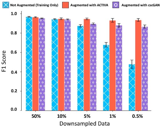
Augmentation with ACTIVA improves classification of rare populations. Mean F1 scores of RF classifier for training data (with no augmentation), shown in blue, and training data with augmentation, shown in red and purple. Error bars indicate the range for five different random seeds for sub-sampling cluster 2 cells.

6 Conclusions and discussion

In this manuscript, we propose a deep generative model for generating realistic scRNAseq data. Our model, ACTIVA, consists of an automatic cell-type identification network, coupled with IntroVAE that aims to learn the distribution of the original data and the existing sub-populations. Due to the architectural choices and single-stream training, ACTIVA trains orders of magnitude faster than the state-of-the-art GAN-based model, and produces samples that are comparably in quality. ACTIVA can be easily trained on different datasets to either enlarge the entire dataset (generate samples from all clusters) or augment specific rare populations.

ACTIVA can generate hundreds of thousands of cells in only a few seconds (on a GPU), which enables benchmarking of new scRNAseq tools’ accuracy and scalability. We showed that, for these datasets, using ACTIVA for augmenting rare populations improves downstream classification by more than 40% in the rarest case of real cells used (0.5% of the training samples). We believe that ACTIVA learns the underlying higher-dimensional manifold of the scRNAseq data, even where there are few cells available. The deliberate architectural choices of ACTIVA provide insights as to why this learning occurs. As Marouf et al. (2020) also noted, the fully connected layers of our three networks share information learned from all other populations. In fact, the only cluster-specific parameters are the ones learned in the batch normalization layer. This is also shown with the accuracy of the conditioner network when trained on rare populations. However, if the type-identifying network does not classify sub-populations accurately, this can directly affect the performance of the generator and inference model due to the conditioning. We keep this fact in mind and therefore allow for the flexibility of adding any classifier to our existing architecture. Given our architecture, we hypothesize that the conditioner network could be used directly as the encoder, or its learned parameters could be transferred to the encoder network, which we plan to explore in the future.

Lopez et al. (2018) demonstrate that the latent manifold of VAEs can also be useful for analyses such as clustering or denoising. Deep investigation of the learned manifold of ACTIVA can further improve the interpretability of our model, or yield new research questions to explore. We also hypothesize that assuming a different prior such as a Zero Inflated Negative Binomial or a Poisson distribution could further improve the quality of generated data. Our experiments show that ACTIVA learns to generate high-quality samples on complex datasets from different species. ACTIVA potentially reduces the need for human and animal sample sizes and sequencing depth in studies, saving costs and time, and improving robustness of scRNAseq research with smaller datasets. Furthermore, ACTIVA would benefit studies where large or diverse patient sample sizes are not available, such rare and emerging disease.

Funding

The authors were support from the National Institutes of Health [R15-HL146779 & R01-GM126548], National Science Foundation [DMS-1840265] and University of California Office of the President and University of California Merced COVID-19 Seed Grant.

Conflict of Interest: none declared.

References

- Abdelaal T. et al. (2019) A comparison of automatic cell identification methods for single-cell RNA sequencing data. Genome Biol., 20, 194. [DOI] [PMC free article] [PubMed] [Google Scholar]
- Arjovsky M., Bottou L. (2017) Towards principled methods for training generative adversarial networks. In: International Conference on Learning Representations, arXiv, 1701.04862. [Google Scholar]
- Arjovsky M. et al. (2017) Wasserstein generative adversarial networks. Proc. Mach. Learn. Res., 70, 214–223. [Google Scholar]
- Assefa A.T. et al. (2020) SPsimSeq: semi-parametric simulation of bulk and single-cell RNA-sequencing data. Bioinformatics, 36, 3276–3278. [CrossRef][10.1093/bioinformatics/btaa105] [DOI] [PMC free article] [PubMed] [Google Scholar]
- Benidt S., Nettleton D. (2015) SimSeq: a nonparametric approach to simulation of RNA-sequence datasets. Bioinformatics, 31, 2131–2140. [CrossRef][10.1093/bioinformatics/btv124] [DOI] [PMC free article] [PubMed] [Google Scholar]
- Button K.S. et al. (2013) Power failure: why small sample size undermines the reliability of neuroscience. Nat. Rev. Neurosci., 14, 365–376. [CrossRef][10.1038/nrn3475] [DOI] [PubMed] [Google Scholar]
- Dziugaite G.K. et al. (2015) Training generative neural networks via maximum mean discrepancy optimization. In: Proceedings of the Thirty-First Conference on Uncertainty in Artificial Intelligence, Amsterdam, Netherlands, AUAI Press, Arlington, Virginia, USA. Pp. 258–267. [Google Scholar]
- Frazee A.C. et al. (2015) Polyester: simulating RNA-seq datasets with differential transcript expression. Bioinformatics, 31, 2778–2784. [DOI] [PMC free article] [PubMed] [Google Scholar]
- Gerard D. (2020) Data-based RNA-seq simulations by binomial thinning. BMC Bioinformatics, 21, 206. [DOI] [PMC free article] [PubMed] [Google Scholar]
- Goodfellow I. et al. (2014) Generative adversarial nets. Adv. Neural Inf. Process. Syst., 27, 2672–2680. [Google Scholar]
- Gretton A. et al. (2012) A kernel two-sample test. J. Mach. Learn. Res., 13, 723–773. [Google Scholar]
- Han X. et al. (2018) Mapping the mouse cell atlas by Microwell-seq. Cell, 172, 1091–1107. [DOI] [PubMed] [Google Scholar]
- He J. et al. (2019) Lagging inference networks and posterior collapse in variational autoencoders. In: International Conference on Learning Representations.
- Heming M. et al. (2021) Neurological manifestations of COVID-19 feature T-cell exhaustion and dedifferentiated monocytes in cerebrospinal fluid. Immunity, 54, 164–175.e6. [DOI] [PMC free article] [PubMed] [Google Scholar]
- Heydari A.A. et al. (2019) SoftAdapt: techniques for adaptive loss weighting of neural networks with multi-part loss functions. CoRR, abs/1912.12355. [Google Scholar]
- Heydari A.A., Mehmood A. (2020) SRVAE: super resolution using variational autoencoders. In: Pattern Recognition and Tracking XXXI. International Society for Optics and Photonics.
- Huang H. et al. (2018) IntroVAE: introspective variational autoencoders for photographic image synthesis. In: Advances in Neural Information Processing Systems, 31. [Google Scholar]
- Kingma D.P., Welling M. (2013) Auto-encoding variational Bayes. In: International Conference on Learning Representations. [Google Scholar]
- Lindenbaum O. et al. (2018) Geometry based data generation. In: Bengio S. et al. (eds.) Advances in Neural Information Processing Systems, vol. 31. Curran Associates, Inc., pp. 1400–1411 [Google Scholar]
- Liu Q. et al. (2019) hicGAN infers super resolution Hi-C data with generative adversarial networks. Bioinformatics, 35, i99–i107. [DOI] [PMC free article] [PubMed] [Google Scholar]
- Lopez R. et al. (2018) Deep generative modeling for single-cell transcriptomics. Nat. Methods, 15, 1053–1058. [DOI] [PMC free article] [PubMed] [Google Scholar]
- Lucic M. et al. (2018) Are GANs created equal? A large-scale study. In: Proceedings of the 32nd International Conference on Neural Information Processing Systems, NIPS’18. Curran Associates Inc., Red Hook, NY, pp. 698–707. [Google Scholar]
- Ma F., Pellegrini M. (2020) ACTINN: automated identification of cell types in single cell RNA sequencing. Bioinformatics, 36, 533–538. [DOI] [PubMed] [Google Scholar]
- Marouf M. et al. (2020) Realistic in silico generation and augmentation of single-cell RNA-seq data using generative adversarial networks. Nat. Commun., 11, 166. [DOI] [PMC free article] [PubMed] [Google Scholar]
- Metz L. et al. (2016) Unrolled generative adversarial networks. In: 5th International Conference on Learning Representations, {ICLR} 2017, Toulon, France, April 24-26, 2017, Conference Track Proceedings, OpenReview.net. [Google Scholar]
- Miyato T., Koyama M. (2018) cGANs with projection discriminator. In: International Conference on Learning Representations.
- Regev A. et al. ; Human Cell Atlas Meeting Participants. (2017) The human cell atlas. Elife, 6, e27041. [DOI] [PMC free article] [PubMed] [Google Scholar]
- Shorten C., Khoshgoftaar T.M. (2019) A survey on image data augmentation for deep learning. J. Big Data, 6, 60. [DOI] [PMC free article] [PubMed] [Google Scholar]
- Tang F. et al. (2009) mRNA-seq whole-transcriptome analysis of a single cell. Nat. Methods, 6, 377–382. [DOI] [PubMed] [Google Scholar]
- Tang X. et al. (2019) The single-cell sequencing: new developments and medical applications. Cell Biosci., 9, 53. [DOI] [PMC free article] [PubMed] [Google Scholar]
- Theis L. et al. (2016) A note on the evaluation of generative models. In: International Conference on Learning Representations.
- Wang Z. et al. (2019) Generative adversarial networks in computer vision: a survey and taxonomy. In: Association for Computing Machinery, New York, NY, USA. https://doi.org/10.1145/3439723. [Google Scholar]
- Zadrozny B. et al. (2003) Cost-sensitive learning by cost-proportionate example weighting. In Third IEEE International Conference on Data Mining, pp. 435–442.
- Zappia L. et al. (2017) Splatter: simulation of single-cell RNA sequencing data. Genome Biol., 18, 174. [DOI] [PMC free article] [PubMed] [Google Scholar]
- Zhang X. et al. (2019) Simulating multiple faceted variability in single cell RNA sequencing. Nat. Commun., 10, 2611. [DOI] [PMC free article] [PubMed] [Google Scholar]
- Zheng G.X.Y. et al. (2017) Massively parallel digital transcriptional profiling of single cells. Nat. Commun., 8, 14049. [DOI] [PMC free article] [PubMed] [Google Scholar]
- Zheng K. et al. (2020) Conditional introspective variational autoencoder for image synthesis. IEEE Access, 8, 153905–153913. [Google Scholar]
Associated Data
This section collects any data citations, data availability statements, or supplementary materials included in this article.