Blind demixing methods for recovering dense neuronal morphology from barcode imaging data

Shuonan Chen; Jackson Loper; Pengcheng Zhou; Liam Paninski

doi:10.1371/journal.pcbi.1009991

. 2022 Apr 8;18(4):e1009991. doi: 10.1371/journal.pcbi.1009991

Blind demixing methods for recovering dense neuronal morphology from barcode imaging data

Shuonan Chen ^1,^2,^3,^4,^5,^6,^*, Jackson Loper ^1,^2,^3,^4,^5,⁷, Pengcheng Zhou ^8,⁹, Liam Paninski ^1,^2,^3,^4,^5,⁷

Editor: Hermann Cuntz¹⁰

PMCID: PMC9020678 PMID: 35395020

Abstract

Cellular barcoding methods offer the exciting possibility of ‘infinite-pseudocolor’ anatomical reconstruction—i.e., assigning each neuron its own random unique barcoded ‘pseudocolor,’ and then using these pseudocolors to trace the microanatomy of each neuron. Here we use simulations, based on densely-reconstructed electron microscopy microanatomy, with signal structure matched to real barcoding data, to quantify the feasibility of this procedure. We develop a new blind demixing approach to recover the barcodes that label each neuron, and validate this method on real data with known barcodes. We also develop a neural network which uses the recovered barcodes to reconstruct the neuronal morphology from the observed fluorescence imaging data, ‘connecting the dots’ between discontiguous barcode amplicon signals. We find that accurate recovery should be feasible, provided that the barcode signal density is sufficiently high. This study suggests the possibility of mapping the morphology and projection pattern of many individual neurons simultaneously, at high resolution and at large scale, via conventional light microscopy.

Author summary

In situ barcode sequencing allows us to simultaneously locate many neurons in intact brain tissues, albeit at modest spatial resolution. By increasing the barcode density, high-resolution neuronal morphology reconstruction from such data might be possible. Here we use simulations to study this possibility, while addressing the computational challenges in analyzing such data. We developed a novel blind demixing method that uses fluorescent images and identifies the unknown barcodes used to label the neurons with high accuracy. Further, we developed a neural network which can reconstruct the morphology for these labeled neurons from the observed ‘pointilistic’ imaging data. We show that under both high- and low-resolution optical settings, our methods can successfully extract the morphologies for many labeled neurons. The results from this theoretical study suggest that it may be feasible to map the morphology and projection pattern of many individual neurons simultaneously, at high resolution and at large scale, via conventional light microscopy.

1 Introduction

Neuroscientists have long dreamed of obtaining simultaneous maps of the morphology of every neuron in a mammalian brain [1, 2]. The ability to perform this very high-throughput neuron-tracing would enable better understanding of brain development, neural circuit structure, and the diversity of morphologically-defined cell types [3, 4]. In order to map the morphology at the scale of a mammalian brain, an ideal experiment would trace a large number of neurons simultaneously over a large brain region with high imaging resolution.

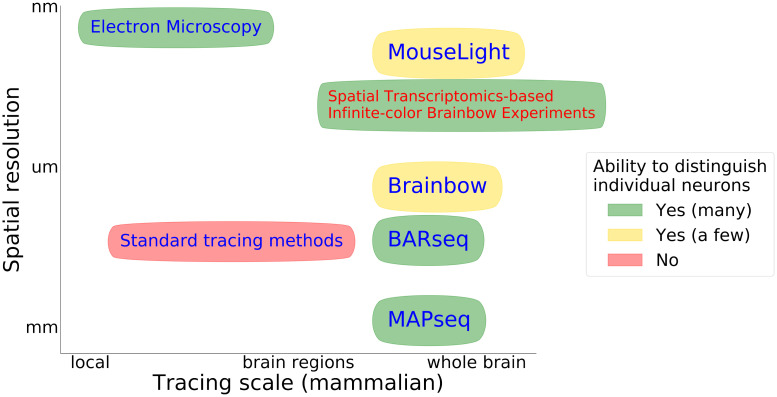
Current experimental methods for neuronal tracing can be placed along a spectrum spanning two disparate spatial scales. On the one hand, techniques based on Electron Microscopy (EM) obtain nanometer-level resolution within small regions. On the other hand, light microscopy and molecular techniques can map morphology over whole-brain scales, albeit with relatively low spatial resolution and/or limitations on the number of neurons that can be mapped simultaneously. Fig 1 sketches the current landscape, and highlights a gap in the state of the art: mapping many neurons simultaneously, with high resolution, over large fields of view (or potentially even the whole brain).

Fig 1 — Here we non-exhaustively summarize the landscape of existing neuronal tracing methods. The horizontal axis indicates the typical scale of these neuronal tracing methods, ranging from local tracing to mapping axonal projections across the whole brain; the vertical axis indicates optical resolution in the typical images obtained from these methods. The ellipse color represents the number of neurons that can be traced and distinguished; red indicates that the method cannot readily distinguish between spatially nearby neurons, yellow indicates that the method can be used to trace several individual neurons, and green indicates the possibility of simultaneously mapping thousands or millions of neurons. Here ‘standard tracing methods’ refer to approaches such as Golgi staining and viral tracers; cf. Section 2 for more details. Note that many of these methods rely on conventional optical microscopes, and their resolution can potentially be increased via expansion microscopy and/or super resolution microscopy, though this may incur additional experimental costs. In this paper we focus on the possibility of extending molecular barcoding methods by increasing the signal density to allow for more fine-grained morphological reconstructions; we call such experiments Spatial Transcriptomics-based Infinite-color Brainbow Experiments (STIBEs).

Molecular barcoding methods may be able to fill the gap [5, 6] with ‘infinite-color Brainbow’ experiments: each cell is labeled with a unique random barcode which can be visualized through conventional light microscopy. If we think of each barcode as providing a unique ‘pseudocolor’ for each cell, then conceptually this method ‘colors’ the brain with a potentially unbounded number of random colors, generalizing the original Brainbow approach [7], which can trace long-range neuronal morphology but was limited to a relatively small number of random colors (though see e.g. [8] for more recent developments).

Here we use simulations to investigate a class of methods we dub Spatial Transcriptomics-based Infinite-color Brainbow Experiments (STIBEs). Can such experiments obtain precise morphological reconstruction? Can we potentially obtain long-range tracing for many neurons simultaneously, if the experiment is done at a sufficienctly large scale? This class of experiments uses techniques from the spatial transcriptomics community to label cells with unique fluorescent barcodes, in-situ; the BAR-seq method is a representative example [5]. STIBEs work by creating a collection of transcripts containing barcode sequences; these transcripts are amplified into target molecules known as ‘amplicons,’ and the barcode associated with each amplicon can be identified over a series of rounds of imaging. In an ideal STIBE, all amplicons within a given cell carry the same barcode, no two cells carry amplicons with the same barcode, and amplicons are only present within cells. By identifying collections of amplicons which carry the same barcode, one can thus trace many neurons across the entire brain.

Previous experiments have already demonstrated that STIBEs can be used to recover the locations of somas and projection sites of many cells (at lower spatial resolution) [5, 9]. In contrast, here we focus on STIBEs that could achieve micron-resolution morphological reconstruction of many cells simultaneously, potentially across the whole brain. This would be a valuable advance for several reasons. First, cell morphology measured at this scale provides a great deal of information about cell type in different layers and regions of the brain [10, 11]. Second, although micron-level resolution does not permit exact connectome reconstruction, it does yield a matrix of potential connections between neurons (i.e., which cells might be connected to each other). Such matrices would be invaluable for downstream applications such as functional connectivity mapping (by providing constraints on possible connections) [12] or cell type inference [13–15].

To accurately simulate the imagestacks that would be generated by STIBEs, we use two sources of existing data. First, we use densely-reconstructed EM data to give us the shapes and spatial relationships between axons and dendrites in a small cortical volume. Second, we replicate the noise and signal structure we might expect, based on results from current cellular barcoding experiments [5, 6]. We investigate how varying parameters of STIBEs would affect the accuracy of neuronal tracing; for example, we consider various imaging resolutions and various densities of the amplicons present within cells. We find that selecting an appropriate density of amplicons is a balancing act: we cannot recover precise morphological reconstructions without sufficient density, but very high density can lead to incorrect amplicon identification along thin processes due to limited optical resolution.

Our main technical contribution here is to develop improved demixing algorithms that enable improved barcode recovery in the high-density regime, leading in turn to improved morphological recovery. These algorithms are based on the BarDensr model of spatial transcriptomics data [16] (see also [17], as well as [18, 19]), which was originally developed to detect barcode signals from spatial transcriptomics images when the barcode library is known. We have extended this method to a more challenging ‘blind demixing’ setting, where we iteratively learn the barcodes directly from the available image data, so that it is applicable to STIBEs where the barcode library is unknown or intractably large. We further developed a Convolutional Neural Network (CNN) model to reconstruct morphology for each demixed barcode, ‘connecting the dots’ between the discontiguous fluorescent signals produced by amplicons.

In what follows, we contextualize STIBEs among the family of other neuronal tracing methods, describe our methods for simulation and image analysis, and finally report our findings on the feasibility of STIBEs for the morphological reconstruction of neurons.

2 Related work

The history of neuronal tracing techniques is long and complex [20]; here we give a brief overview of some techniques most directly relevant to our approach. Fig 1 presents a visual overview.

At one extreme of the precision-scale spectrum, Electron Microscopy (EM) is the state-of-the-art tool for visualizing a small region of brain with very high precision [14, 15, 21–25]. However, it is not yet suitable for dense mapping of long-range neuronal projections: the imaging (and computational segmentation) process for these experiments is challenging, and it is not yet feasible to use EM to densely trace many neurons across the mammalian brain. It may be possible to refine EM techniques to overcome these challenges, but this is not our focus in this paper (cf. [2] for further discussion).

At the opposite extreme of the precision-scale spectrum, we have standard tracing approaches utilizing light microscopy. Despite significant effort [26], it remains infeasible to segment and trace thousands of densely-packed individual neurons visualized with a single tracing marker. The ‘MouseLight’ project [27] is a modern exemplar of this ‘classical’ approach. This is a recently developed platform for tracing the axonal arbor structure of individual neurons, built upon two-photon microscopy and viral labeling of a sparse set of neurons, allowing long-range neuronal tracing. Unfortunately, the number of neurons that can be traced at once is currently limited to a hundred per brain sample [28] (though more advanced microscopy technology, such as super-resolution microscopy [29–33], and/or Expansion Microscopy [34–37], could potentially be deployed to simultaneously trace more individual neurons with higher resolution).

‘Brainbow’ methods [7, 38] introduce random combinations of fluorescent markers to facilitate tracing of multiple cells. The number of neurons that can be uniquely labeled and identified by the original method was limited to several hundreds, because of limitations on the number of distinct colors that can be generated and distinguished. Recent studies have focused on reducing these bottlenecks [8, 39, 40], and developing improved computational methods [41, 42].

More recently, molecular barcoding methods have been developed to effectively remove this bottleneck on the number of distinct unique ‘color’ labels that can be assigned and read from different cells. Multiplexed Analysis of Projections by Sequencing (MAPseq) is one early example of this approach, developed to study long-range axonal projection patterns [9]; however, the spatial precision of this approach was not sufficient to capture neuronal morphology. More recently, “barcoded anatomy resolved by sequencing” (BARseq) [5, 6] combines MAPseq and in situ sequencing technology to obtain higher spatial resolution. Instead of micro-dissecting the brain tissue, this method uses fluorescent microscopy to detect the barcode signal from the intact tissue, similar to recent spatial transcriptomics methods [43, 44]. In theory, BARseq should be capable of satisfying all the desirable features of neuronal tracing: uniquely labelling large numbers of individual neurons, representing them with high spatial precision, and tracing them across long distances through the brain. Spatial transcriptomics technology is advancing quickly; for example, [45] recently achieved single-cell-resolution transcriptomic assays of an entire embryo. As this technology advances, techniques like BARseq can only become more effective. However, to date, this technology has only been used with a relatively small number of amplicons per cell, prohibiting accurate morphological reconstruction (c.f. Brainbow images, where signal within cells tends to be much more uniform and less ‘pointilistic,’ leading to a different class of segmentation problems). In theory, there is nothing preventing new experiments with higher density, to achieve higher-resolution morphology mapping; this paper will explore this idea systematically.

Finally, we note the related paper [46]; this previous simulation work focused on a different experimental context, specifically expansion microscopy and cell membrane staining with fluorescent markers. In the current work we are interested in exploring the frontier of morphology mapping using only molecular barcoding images and conventional light microscopy. Introducing expansion microscopy and additional fluorescent labels could potentially improve the resolution of the methods studied here, at the expense of additional experimental complexity.

3 Methods summary

We here summarize the three main procedures used in this work; full details can be found in S1A Appendix.

3.1 Data simulation

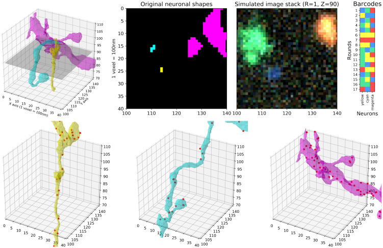
In order to investigate feasible experimental conditions for densely reconstructing neuronal morphology, we simulated a variety of STIBEs. The simulation process is illustrated in Fig 2. We started with densely segmented EM data [14, 15, 47]. Next we generated a random barcode library, assigning random barcodes to each cell in the field of view (FOV). We simulated amplicon locations according to a homogeneous Poisson process within the voxelized support of each cell. The final imagestack was generated by assigning a colored spot to each barcode location in each imaging frame, and then pushing the resulting high-resolution 3D ‘clean’ data through an imaging model that includes blurring with a point spread function, sampling with a lower-resolution voxelization, and adding imaging noise, to obtain the simulated observed imagestack.

Fig 2 — **Top left**: Three neuronal segments in a small region (40 × 40 × 40 voxels with 100 × 100 × 100 nm voxel size). The original EM data is much more densely packed than what is shown here; for illustration purposes, we only show three neurons among many. **Top middle**: A 2D slice with each neuronal segment uniquely colored (left) and the simulated imagestack at the same plane for the first sequencing round (right). The imagestack colors do not correspond to neural segment colors, but rather to the corresponding fluorescent barcodes (top right). A video corresponding to this plot, showing multiple z-planes, can be found at this link. **Bottom**: Amplicons are uniformly simulated within neuronal segment volumes; simulated amplicons are shown as red dots.

3.2 Barcode estimation

To use a STIBE for morphological reconstruction, one must estimate the barcodes present in a FOV (each barcode corresponding to one cell) and the locations of each amplicon corresponding to each barcode (these amplicon locations pointilistically trace the morphology of each cell). The barcode library used to infect the neurons is unknown in such data. In theory, one could sequence the viral library, but this may yield a set of barcodes which is too large to be useful [48]. For the purpose of morphology reconstruction—where only a small number of cellular barcodes exist in a region of interest—we must develop an approach to ‘learn’ the local barcode library from the images themselves. We found that there are effectively two distinct regimes for barcode and amplicon recovery. In the ‘sparse’ regime, where imaging resolution is high and the amplicon density is low, the signal in most imaging voxels is dominated by at most one amplicon. Thus we can estimate the barcode library simply by searching for bright, ‘clean’ imaging voxels displaying a single amplicon signal to estimate the amplicon locations using the resulting barcode library. In the ‘dense’ regime (with high amplicon density and/or low imaging resolution) it is harder to find voxels dominated by a single amplicon, and the simple approach described above breaks down. Instead, we have found that an iterative constrained non-negative matrix factorization approach is more effective: given an initial (incomplete) estimate of the barcode library, we estimate the corresponding amplicon locations, then subtract away the estimated signal corresponding to these amplicons. This sparsens the remaining image, making it easier to detect more barcodes that might have been obscured in previous iterations. After augmenting the barcode library with these previously undetected barcodes, we can re-estimate the amplicon locations and iterate between these two steps (updating the barcode library and estimating amplicon locations in alternating fashion) until a convergence criterion is satisfied. This approach takes full advantage of our knowledge of the special structure of this blind-demixing problem; classic blind-demixing approaches (e.g. regular non-negative matrix factorization) that do not exploit this problem structure do not perform well here.

3.3 Amplicon estimation and morphological reconstruction

Given an estimated barcode library, our primary goal is to reconstruct the morphology of each neuron labeled by a barcode in this library. Our starting point in this endeavor is the ‘evidence tensor’ (see S1 Appendix for a precise definition), which summarizes our confidence about the presence of each barcode at each voxel location. This evidence tensor is used as the input to two algorithms: alphashape [49] and Convolutional Neural Networks (CNNs), which are trained to estimate the shape of each neuron from the evidence tensor.

4 Results

Below we report our ability to recover barcodes and reconstruct morphology in two different simulation regimes: the ‘high-resolution, dense-expression’ regime, in which every neuron is labeled and imaged with sub-micron resolution; and the ‘low-resolution, sparse-expression’ regime, in which only about 1% of neurons are labeled and imaged with micron-resolution imaging. The first regime (‘high-resolution simulation’ for short) represents an ideal setting. For this regime, we also used real experimental data to test if the barcode recovery method works on real-world data with a known set of barcodes. Experiments in the second regime (‘low-resolution simulation’ for short) would be considerably cheaper to perform, with lower optical resolution facilitating faster image acquisition over large FOVs; however, the resolution in this simulation is low enough that many cellular barcodes may occupy a single voxel. To enable accurate recovery in this regime we must also assume that the cell capture efficiency is relatively low: i.e., only a fraction of neurons express a barcode.

4.1 High-resolution, dense-expression simulations

In our first set of simulations, we assume diffraction-limited imaging with an isotropic point spread function (PSF). We further assume that the viral infection has a perfect efficiency; in this extreme case, all the neurons captured by EM in this brain region are labeled with a unique barcode. The simulation process is illustrated in Fig 2. With these assumptions fixed, we investigated a range of experimental parameters, varying the amplicon density as a key parameter of interest. We denote this density by λ and measure it with units of amplicons per cubic micron of neuronal volume. We investigated densities from 1 amplicon per cubic micron (i.e., λ = 1) to 200 amplicons per cubic micron (i.e., λ = 200). For each density variant we investigated our ability to recover barcodes. The simulation results using three of these densities (1, 10 and 100 amplicons/μm³) are summarized in Fig 3. More details on the simulation process can be found in S1A.1 Appendix.

Fig 3 — **Left**: 2D slice of the original neuronal shapes; each neuron is visualized with a different random color. Partial overlapping due to point-spread blur can be seen from the mixing of the colors on the boundary of the neurons. **Right**: Corresponding slice of the simulated imagestack, considering several different density values. Note that the imagestack colors do not correspond to the neuronal visualization colors on the left; the imagestack colors arise from their corresponding barcodes. A video showing multiple z-planes can be found at this link.

4.1.1 Barcode estimation

To estimate the barcode library present in a STIBE, we take advantage of a special structure in the barcodes of typical spatial transcriptomics experiments: each fluorescent barcode is designed so that exactly one channel is active in each imaging round. This suggests a simple approach for recovering the barcode library: search for voxels where one channel is much brighter than all others in every round. This approach is successful in some cases. Barcode discovery using this simple approach is easiest with a medium density of amplicons. In the low-density case, with λ = 1 amplicon/μm³, we were able to find 847 out of 975 barcodes present in tissue using this naïve approach, representing a detection rate of 86.87%, with 0 false positives (however, as we discuss later, our ability to reconstruct neuronal morphology in this low-density case is quite limited). Increasing the density to 10 transcripts per cubic micron (λ = 10 amplicons/μm³), we are able to detect 945 barcodes (96.92% detection rate) with 2 false positives. Note that barcode recovery rates drop in the very low amplicon density regime, since some small cells in the FOV may not express enough amplicons for reliable detection. (Of course in practice a user may wish to adjust the detection threshold according to their own needs, since the relative cost of a false negative versus false positive will likely vary across different experimental conditions).

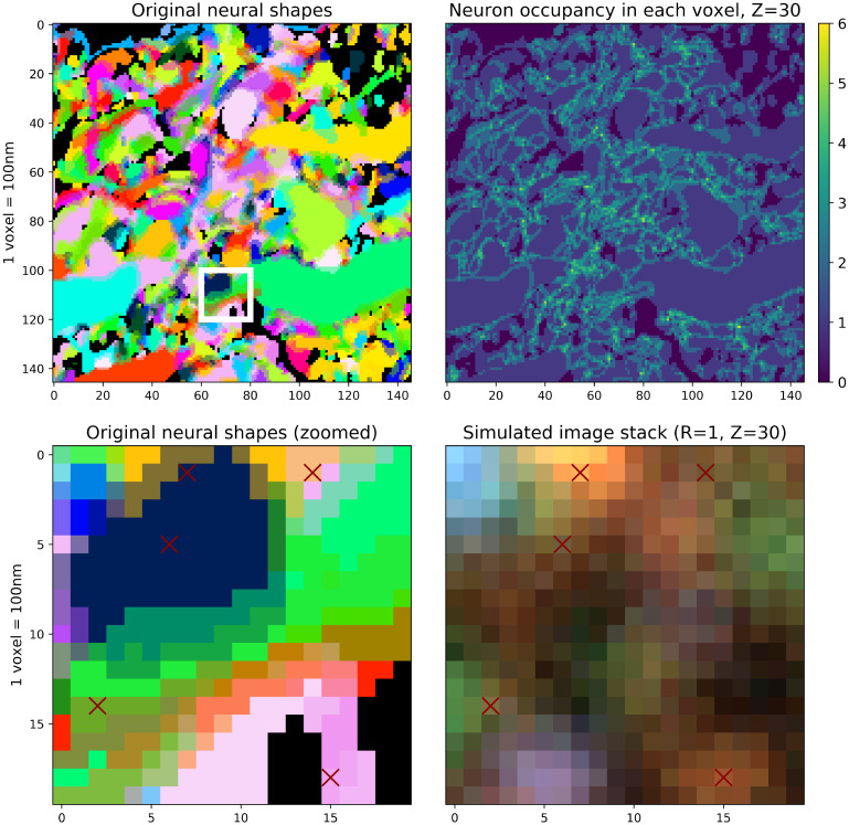
As shown in Fig 4, even with medium density the signal can be significantly mixed; that is, a single voxel can display signal from multiple cells, even under the assumption of high-resolution imaging system. When this occurs, correctly identifying the barcodes becomes challenging even manually. Increasing the density further to 100 transcripts per cubic micron (λ = 100 amplicons/μm³), this problem becomes severe: the naïve method can detect only 604 barcodes, representing a detection rate of 61.95%, with zero false positives.

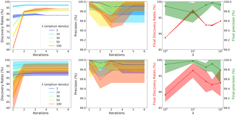
In short, we found the naïve barcode recovery method inadequate when the amplicon density is high, even under idealistic assumptions on optical resolution. In order to recover most of the barcodes, we need to demix the accumulated signal emitted by many barcodes contributing to a single voxel. We adopted a novel iterative approach based on non-negative matrix factorization, detailed in S1A.2.2 Appendix and Algorithm 3. The results of this iterative barcode discovery approach under different amplicon densities are shown in Fig 5. Here, we generated two types of datasets, shown on the top and the bottom panels respectively. The first type of dataset was simulated from a single EM volume, and the second type was simulated from different EM volumes. For the first type, we simulated five random datasets from a single EM volume, using a wide range of amplicon densities. In this case, the randomness applies to both codebook and spot locations within the cell region, but all the datasets share the same ground-truth neuronal regions. For the second type, five different EM subvolumes are used to generate five random datasets. In this case, each of these five datasets has a different ground-truth neuronal region. In all cases we chose the parameters to ensure at most five total false positives throughout the iterations, to maintain a high level of precision throughout. This was done by increasing the signal_control value (see S1A.2.1 Appendix) until the false positives stayed below five throughout all iterations; a high value of this parameter leads to a more conservative discoveries. We found that 2–3 iterations consistently improve performance, yielding 30% more detections when the amplicon density is very high (λ = 100 amplicons/μm³).

Fig 5 — **Top**: five datasets are randomly simulated from a single EM volume and performances are summarized here. The left panel shows barcode discovery rate, as a fraction of the 975 neurons present in the original EM volume. The middle panel shows the precision at each iteration, which is the proportion of True Positives among all the positive detections. These two panels show these metrics evaluated on STIBEs with various densities of amplicons (λ, colored lines) analyzed using different numbers of iterations. The shaded regions for each line indicate the standard deviation. We see that multiple iterations improve recovery accuracy when the density of amplicons is high. The right panel shows the final discovery rate (vertical axis on the left, red) as well as the final precision (vertical axis on the right, green) after six iterations, as a function of amplicon density (at log-scale, horizontal axis). Recovery accuracy peaks at λ values around 10 amplicons/μm³, where amplicons are neither too dense (where too much optical overlap leads to decreases in recovery accuracy) nor too sparse (where there is simply not enough information to recover some barcode identities). **Bottom**: five datasets are randomly simulated from five different EM volumes and the performances are summarized here. The plots are arranged in the same way as above. Here we see a very similar trends, albeit with larger variations across the replicates, confirming the results generalize across multiple FOVs. These plots further confirmed that 10 amplicons/μm³ is an optimal value for this iterative barcode discovery task, under these simulated imaging conditions.

In summary, in our high-resolution setting, we can accurately detect the barcode library using the naïve approach when the signal density is relatively low. On the other hand, when the signal density is high, we can still recover most of the barcodes correctly by using the iterative approach.

4.1.2 Real experimental data barcode estimation

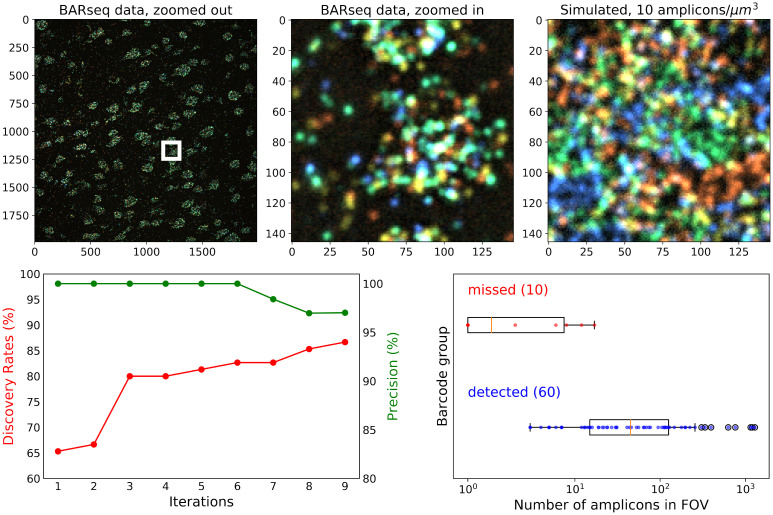
In order to test our method on real-world data, we used benchmarking data from a previous study [16], where the barcodes are used to identify genes rather than cells. In this experiment, the barcodes are known beforehand; we can use these barcodes as the ground-truth codebook, and attempt to recover this codebook. Note that because the barcodes correspond to genes instead of cells, we are not able to use this dataset to benchmark cellular morphology reconstruction results. Fig 6 (top panel) displays a comparison of this real experimental data against our simulated data; we see a reasonable correspondence between the simulated and real data here, in terms of both the expression density and image signal-to-noise ratio.

Fig 6 — **Top**: An example image from the first round of imaging is shown on the left panel. The middle panel is a zoomed-in view of the white rectangle on the left. On the right panel, we showed the simulated data with 10 amplicons/μm³ density to show that our simulation corresponds reasonably well to the real experimental data. **Bottom**: The result of iterative barcode discovery on the entire FOV shown on the left top panel. The discovery rate (red) and precision (green) over each iteration are shown on the left plot. We also investigated if there is an association between the barcode detection accuracy and the number of amplicons in the image that belong to that barcode. On the right panel, we show that all missed barcodes are associated with small numbers of amplicons; barcode detection can be achieved as long as we have a sufficiently large number of amplicons present in the FOV.

In this ground-truth codebook, we have 79 barcodes used to target mRNAs, and 70 of them had at least one amplicon in the images (the number of amplicons are estimated using BarDensr [16], which utilizes the known barcode library). As in the simulations above, we applied the naïve barcode discovery approach first. Using the naïve approach we could only detect 65.3% of all the barcodes with at least one amplicon. Using the iterative approach, the detection rate increased to 86.7%, as shown in Fig 6 bottom left. (For details on the barcodes estimated using real data, see S1 A.2.3 Appendix) The few missed barcodes here (i.e., False Negatives) tend to correspond to targets with relatively small numbers of amplicons in the FOV (Fig 6 bottom right). Two examples of missed barcodes are shown in S2 Fig. Note that this experiment was performed with only six imaging rounds (rather than 17 imaging rounds used in our simulation settings) and these shorter barcode sequences lead to higher error rates than seen in the simulated results.

4.1.3 Amplicon estimation and morphological reconstruction

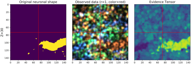
In order to estimate the morphology corresponding to each recovered barcode, we start by estimating the density of each barcode at each voxel; we refer to this estimate as the ‘evidence tensor’ (cf. S1A.3 Appendix). Note that this ‘evidence tensor’ is computed using barcodes recovered from the imagestack (rather than the ground-truth barcodes used for creating the simulations). Fig 7 compares the original neuronal shape and the corresponding evidence tensor; we see that the evidence tensor can roughly capture the shape of the original neuron.

Fig 7 — The ground-truth morphology at a selected z-plane for an example neuron is shown on the left; an imagestack from one round at the corresponding z-plane (λ = 10 amplicons/μm³) is shown in the middle; on the right, the corresponding z-plane of the evidence tensor for the barcode corresponding to the neuron on the left is shown. Note that the evidence tensor is bright around the locations of the underlying neuron, as desired. A video of this image (across z-planes) can be found at this link.

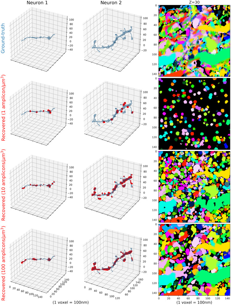
We also investigated neuronal tracing using the estimated evidence tensor with low, medium and high-density variations in Fig 8. The binarized evidence tensors computed from medium-density variation can capture the original morphology relatively well, by correctly identifying the amplicon locations (the third row). However, those learned from low-density variations cannot capture the original morphology as clearly (the second row). The rough path of the neuron can still be identified, but spines are generally missed from dendrites and sub-micron resolution is not achieved. The high-density variation results were similar to the medium-density variation, but with more continuous shape reconstruction (the bottom row). However, they tend to miss the detailed shapes, as well as a portion of the barcodes, due to overlaps of the simulated amplicons in such high-density images. Note here that the evidence tensors are not created to recover the individual amplicon locations but rather to aid in high fidelity reconstructions of the neuronal morphology. High values of this tensor indicates potential amplicon locations, but the set of locations where such high values are achieved is generally larger than the set of locations where amplicons reside (due to blurring induced in the imaging process).

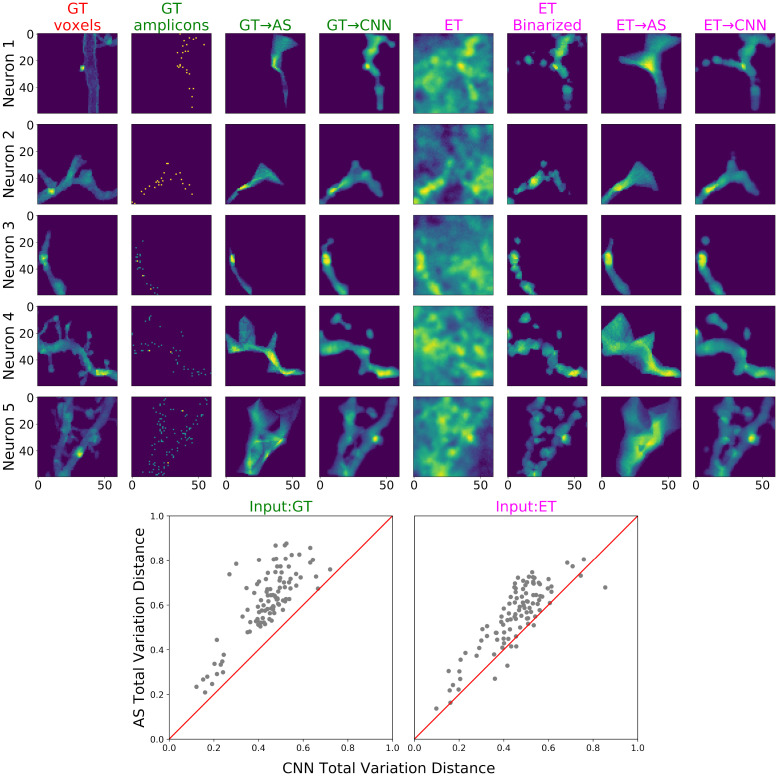
Next we want to estimate the morphology of each neuron from the evidence tensor. We experimented with two approaches here. The first approach applies the alphashape algorithm [49] to a thresholded version of the evidence tensor; this enables better reconstruction of thin portions of the neuron by incorporating our knowledge that neurons occupy contiguous regions in space. Alphashape is a classical method to reconstruct morphology from a point cloud, obtained by computing Delaunay simplices and removing simplices with large circumradii. Fig 9 demonstrates that alphashape is able to estimate the continuous shape of neurons by ‘connecting the dots’ in the evidence tensor. However, it tends to over-estimate the shape, perhaps because alphashapes can only construct linear connections between pairs of detected signals. The second approach uses Convolutional Neural Networks (CNNs) applied to the evidence tensor. This method outperforms alphashape, as shown in Fig 9.

Fig 9 — **Top**: Morphology prediction results for 5 examples. All the columns show the sum-projections across z-planes. The first column shows the ground-truth morphology. The next three columns show the prediction results using alphashape or CNN, when the ground-truth amplicons are used as input (indicated in green titles). The following four columns show the prediction results using alphashape or CNN, when the evidence tensors are used as input (indicated in magenta titles). Evidence tensors are first calculated using the correlation method described in S1A.3.1 Appendix, and before input into alphashape, they are binarized with threshold 0.7, as shown (again, see S1 Fig for details on the choice of this threshold). **Bottom**: Total variation distance (see S1A.3.2 Appendix) on 100 testing examples, including the five shown on the top panel, comparing the results from alphashape prediction on the input (y-axis) and CNN prediction on the input (x-axis). Each dot represents one testing example. The red lines indicate where the two methods have the same performance. Lower values are better; the CNN significantly outperforms the alphashape reconstructions here. A video of the reconstruction result (across z-planes) can be found at this link.

In summary, morphological tracing is difficult with low-density STIBEs, but with sufficient density it is feasible to achieve sub-micron resolution. A thresholded version of the evidence tensor creates a satisfactory summary of the morphology, but it takes the form of a collection of discontiguous regions. To incorporate our knowledge that neurons occupy contiguous regions in space, we can use alphashape (which incorporates this knowledge directly) or CNNs (which learn from data); CNNs yield the best estimates.

4.2 Low-resolution, sparse-expression simulations

Next we investigate whether data from lower-resolution optical systems can still be used to reconstruct neuronal morphology. Here, we assume the optical system is less sensitive: the resolution is lower and the PSF is larger. We also assume the viral infection rate is lower, infecting only 1% of all the axonal segments and discarding all dendritic segments (emulating barcode injection at one site and axonal tracing at another site). This lower infection rate more closely mimics the low labeling efficiency by the current viral barcoding technologies. We assume amplicons can be produced with a density that is roughly consistent with the current experimental technologies, namely 0.08 amplicons per micron length [5]. More details on the low-resolution simulation can be found in S1A.1 Appendix.

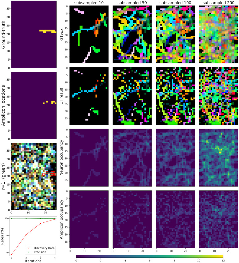
The left column of Fig 10 illustrates the difficulties in analyzing this kind of STIBE. The low optical resolution and high amplicon density often cause multiple amplicons belonging to different axons to occupy the same voxel. The original colors of the target barcodes blend with the other barcodes located nearby in the original physical space, making it difficult to accurately estimate the barcodes associated with cells in a given region of tissue. (Compare this figure with the high-resolution data shown in the middle panel of the top plot of Fig 8, where colors for individual axon targets can be clearly seen).

4.2.1 Barcode estimation

For this dataset, first we applied the same naïve barcode discovery approach that we used for the high-resolution simulations. This naïve method was able to find less than 40% of all the barcodes in the imagestack (assuming a maximum false discovery of 3 barcodes). Therefore, we adopted the iterative approach that was used in high-resolution high-density regime. As shown in the bottom plot of the left panel of Fig 10, four iterations of this approach were sufficient to find all the barcodes (412 in total) for this data, achieving 100% discovery rate with only 1 false positive. This result suggests that even in this more challenging low-resolution regime, an iterative approach can nonetheless recover the barcode library accurately.

4.2.2 Amplicon estimation and morphological reconstruction

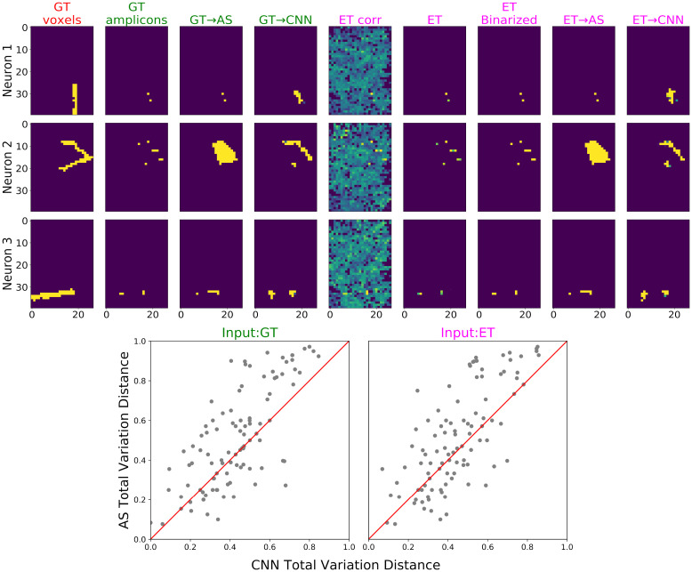
Neuronal tracing on this low-resolution simulation was performed using a similar approach to that taken on the high-resolution dataset. For this dataset, as shown in the top panel of Fig 11, the original evidence tensor already recovers the true amplicon locations quite accurately; a thresholded evidence tensor yields an adequate (though discontiguous) representation of the path of each neuron (see S1 Fig for details on the choice of this threshold). Alphashape or CNN methods can be used to further improve this result, giving reasonable estimates for the contiguous space occupied by each neuron (see Fig 11). All together we see that we are still able to detect the correct morphology of the captured neurons, even for this low-resolution STIBE.

Fig 11 — Similar to Fig 9 for high-resolution simulation, this figure compares morphology reconstructions from low-resolution data using alphashape (AS) and CNN, with ground-truth (GT) amplicons and evidence tensor (ET) as input. Overall, we see that micron-precise morphological reconstructions are possible, even from low-resolution STIBEs. **Top**: Morphology reconstruction results, using either ground-truth amplicons or the evidence tensor as the input to alphashape or CNN. As in Fig 9 the colors of column titles indicate the input categories; from left to right the columns are: the ground-truth morphology, ground-truth amplicons, alphashape and CNN prediction provided ground-truth amplicons as input, evidence tensors using correlation (‘corr’) methods, evidence tensors using amplicon density (described in S1A.3.1 Appendix; note that this is much more accurate than the simple correlation-based method here), thresholded evidence tensor (using amplicon density thresholded at 0.1, see S1 Fig for details on the choice of this threshold), and alphashape and CNN prediction given evidence tensor as input. For the alphashape input, the evidence tensor obtained from amplicon density was binarized with threshold 0.1. **Bottom**: Evaluating the morphology reconstruction using total variation distance loss (see S1A.3.2 Appendix). On the left we show performance using ground-truth amplicon locations (GT, left) and on the right we show performance using the evidence tensor (amplicon density) derived from the imagestack (ET, right); conventions as in Fig 9. CNNs outperform alphashape modestly here.

5 Conclusion

In this work we developed detailed simulations to test the feasibility of using Spatial Transcriptomics-based Infinite-color Brainbow Experiments (STIBEs) for morphological reconstruction of many neurons simultaneously. We developed a novel blind-demixing algorithm, followed by a neural network based reconstruction approach, which together achieve high barcode detection rates and accurate morphological reconstructions, even in relatively low-resolution settings.

There may be room to improve further on the methods proposed here, on at least two fronts. In the first stage, we use an iterative approach to detect barcodes: we model the presence of barcodes that are already in our library, and search the residual images for new barcodes to add to our library. We found that the proposed linear programming approach (building on previous work described in [16]) was effective for decomposing the observed signal into the sum of these two parts (i.e., the signal that can be explained by barcodes we already know and the left over residual), but in future work it may be possible to improve further, using e.g. neural networks trained to decompose images using a simulator similar to the one used here [50].

Second, given an estimated barcode library, we need methods for recovering the morphology corresponding to each barcode from the imagestack. One promising direction would be to use more sophisticated approaches for 3D neuronal recovery, adapting architectures and loss functions that have proven useful in the electron microscopy image processing literature [51, 52]. We hope to explore these directions in future work.

Finally, we should emphasize that this study focused on a small region from a mouse brain, densely reconstructed with electron microscopy. Extending these methods to a whole-brain scale seems feasible but will require significant effort, involving stitching and registering data across many spatial subvolumes analyzed in parallel. As experimental methods continue to march forward and expand in scale [36] we hope to tackle these computational scaling issues in parallel.

Supporting information

S1 Appendix. Detailed methods.

(PDF)

Click here for additional data file.^{(258.4KB, pdf)}

S1 Fig. Finding the threshold for the evidence tensor, for high (top) and low (bottom) resolution data.

In order to create input data for the morphology prediction in Figs 8–11, we needed to binarize the evidence tensors. Here we show the test cases (one row shows one example neuron) where we used various thresholds to binarize the evidence tensors (the third columns and the following) and compared the result with both original ground-truth voxels (first columns), as well as the original (continuous) evidence tensor (second columns). For the high resolution simulation, we used 0.7 as the threshold since the result was robust. This threshold was used to visualize Figs 8 and 9. For the low resolution simulation, we used BarDensr to estimate the evidence tensor and the results were much sparser than the high resolution case, and therefore the binarization was relatively robust to the choice of the threshold. Here we used 0.1 for the low resolution case. This threshold was used to visualize Figs 10 and 11.

(TIFF)

Click here for additional data file.^{(4.2MB, tiff)}

S2 Fig. Missed barcodes in the real data (Fig 6).

Here we show two examples of the amplicons that are from the barcodes that were not found in our amplicon detection process in Fig 6). For both panels, the red frames indicate where the correct barcode signals are expected. The left panel shows the missed barcode which had the most abundant amplicon. We see that the signal intensity varies significantly (e.g., round 2 has much higher signal compared to round 4 and 5). The right panel showed missed barcodes with the third most abundant amplicons. From round 2, 4 and 7 we see there is a relatively high phasing and/or color-mixing happening in the channel 1, which might have made the barcode discovery difficult.

(TIFF)

Click here for additional data file.^{(2.4MB, tiff)}

Acknowledgments

We thank Xiaoyin Chen for sharing the data and helping with the analysis. We thank Li Yuan, Tony Zador, and Abbas Rizvi for many helpful discussions.

Data Availability

The data underlying the results presented in the study is available from https://github.com/jacksonloper/bardensr.

Funding Statement

This work was supported by the National Institutes of Health (1U19NS107613 to L.P.), IARPA MICrONS (D16PC0003 to L.P.), and the Chan Zuckerberg Initiative (2018-183188 to L.P.). The funders had no role in study design, data collection and analysis, decision to publish, or preparation of the manuscript.

References

1.Ramón y Cajal S. Histologie du système nerveux de l’homme & des vertébrés: Cervelet, cerveau moyen, rétine, couche optique, corps strié, écorce cérébrale générale & régionale, grand sympathique. vol. 2. A. Maloine; 1911.
2. Abbott LF, Bock DD, Callaway EM, Denk W, Dulac C, Fairhall AL, et al. The Mind of a Mouse. Cell. 2020;182. doi: 10.1016/j.cell.2020.08.010 [DOI] [PubMed] [Google Scholar]
3. Zador AM, Dubnau J, Oyibo HK, Zhan H, Cao G, Peikon ID. Sequencing the connectome. PLoS Biol. 2012;10(10):e1001411. doi: 10.1371/journal.pbio.1001411 [DOI] [PMC free article] [PubMed] [Google Scholar]
4.Marblestone AH, Daugharthy ER, Kalhor R, Peikon ID, Kebschull JM, Shipman SL, et al. Rosetta brains: a strategy for molecularly-annotated connectomics. arXiv preprint arXiv:14045103. 2014.
5. Chen X, Sun YC, Zhan H, Kebschull JM, Fischer S, Matho K, et al. High-throughput mapping of long-range neuronal projection using in situ sequencing. Cell. 2019;179(3):772–786. doi: 10.1016/j.cell.2019.09.023 [DOI] [PMC free article] [PubMed] [Google Scholar]
6. Sun YC, Chen X, Fischer S, Lu S, Zhan H, Gillis J, et al. Integrating barcoded neuroanatomy with spatial transcriptional profiling enables identification of gene correlates of projections. Nature Publishing Group; 2021. [DOI] [PMC free article] [PubMed] [Google Scholar]
7. Livet J, Weissman TA, Kang H, Draft RW, Lu J, Bennis RA, et al. Transgenic strategies for combinatorial expression of fluorescent proteins in the nervous system. Nature. 2007;450(7166):56–62. doi: 10.1038/nature06293 [DOI] [PubMed] [Google Scholar]
8. Li Y, Walker LA, Zhao Y, Edwards EM, Michki NS, Cheng HPJ, et al. Bitbow: a digital format of Brainbow enables highly efficient neuronal lineage tracing and morphology reconstruction in single brains. bioRxiv. 2020. [DOI] [PMC free article] [PubMed] [Google Scholar]
9. Kebschull JM, da Silva PG, Reid AP, Peikon ID, Albeanu DF, Zador AM. High-throughput mapping of single-neuron projections by sequencing of barcoded RNA. Neuron. 2016;91(5):975–987. doi: 10.1016/j.neuron.2016.07.036 [DOI] [PMC free article] [PubMed] [Google Scholar]
10. Ascoli GA, Donohue DE, Halavi M. NeuroMorpho. Org: a central resource for neuronal morphologies. Journal of Neuroscience. 2007;27(35):9247–9251. doi: 10.1523/JNEUROSCI.2055-07.2007 [DOI] [PMC free article] [PubMed] [Google Scholar]
11. Tasic B, Yao Z, Graybuck LT, Smith KA, Nguyen TN, Bertagnolli D, et al. Shared and distinct transcriptomic cell types across neocortical areas. Nature. 2018;563(7729):72–78. doi: 10.1038/s41586-018-0654-5 [DOI] [PMC free article] [PubMed] [Google Scholar]
12. Stepanyants A, Hof PR, Chklovskii DB. Geometry and structural plasticity of synaptic connectivity. Neuron. 2002;34(2):275–288. doi: 10.1016/S0896-6273(02)00652-9 [DOI] [PubMed] [Google Scholar]
13. Jonas E, Kording K. Automatic discovery of cell types and microcircuitry from neural connectomics. Elife. 2015;4:e04250. doi: 10.7554/eLife.04250 [DOI] [PMC free article] [PubMed] [Google Scholar]
14. Dorkenwald S, Turner NL, Macrina T, Lee K, Lu R, Wu J, et al. Binary and analog variation of synapses between cortical pyramidal neurons. BioRxiv. 2019. [DOI] [PMC free article] [PubMed] [Google Scholar]
15. Schneider-Mizell CM, Bodor AL, Collman F, Brittain D, Bleckert AA, Dorkenwald S, et al. Chandelier cell anatomy and function reveal a variably distributed but common signal. bioRxiv. 2020. [Google Scholar]
16. Chen S, Loper J, Chen X, Vaughan A, Zador AM, Paninski L. Barcode demixing through non-negative spatial regression (bardensr). PLoS computational biology. 2021;17(3):e1008256. doi: 10.1371/journal.pcbi.1008256 [DOI] [PMC free article] [PubMed] [Google Scholar]
17. Andersson A, Diego F, Hamprecht FA, Wählby C. ISTDECO: In Situ Transcriptomics Decoding by Deconvolution. bioRxiv. 2021. [Google Scholar]
18.Bryan JP, Cleary B, Farhi SL, Eldar YC. Sparse Recovery Of Imaging Transcriptomics Data. In: 2021 IEEE 18th International Symposium on Biomedical Imaging (ISBI). IEEE; 2021. p. 802–806.
19. Cleary B, Simonton B, Bezney J, Murray E, Alam S, Sinha A, et al. Compressed sensing for imaging transcriptomics. bioRxiv. 2020; p. 743039. [DOI] [PMC free article] [PubMed] [Google Scholar]
20. Arenkiel BR. Neural Tracing Methods: Tracing Neurons and Their Connections. Neuromethods. Springer; New York; 2014. Available from: https://books.google.com/books?id=RJR1oAEACAAJ. [Google Scholar]
21. White JG, Southgate E, Thomson JN, Brenner S. The structure of the nervous system of the nematode Caenorhabditis elegans. Philos Trans R Soc Lond B Biol Sci. 1986;314(1165):1–340. doi: 10.1098/rstb.1986.0056 [DOI] [PubMed] [Google Scholar]
22. Varshney LR, Chen BL, Paniagua E, Hall DH, Chklovskii DB. Structural properties of the Caenorhabditis elegans neuronal network. PLoS Comput Biol. 2011;7(2):e1001066. doi: 10.1371/journal.pcbi.1001066 [DOI] [PMC free article] [PubMed] [Google Scholar]
23. Oh SW, Harris JA, Ng L, Winslow B, Cain N, Mihalas S, et al. A mesoscale connectome of the mouse brain. Nature. 2014;508(7495):207–214. doi: 10.1038/nature13186 [DOI] [PMC free article] [PubMed] [Google Scholar]
24. Kasthuri N, Hayworth KJ, Berger DR, Schalek RL, Conchello JA, Knowles-Barley S, et al. Saturated reconstruction of a volume of neocortex. Cell. 2015;162(3):648–661. doi: 10.1016/j.cell.2015.06.054 [DOI] [PubMed] [Google Scholar]
25.Turner NL, Lee K, Lu R, Wu J, Ih D, Seung HS. Synaptic partner assignment using attentional voxel association networks. In: 2020 IEEE 17th International Symposium on Biomedical Imaging (ISBI). IEEE; 2020. p. 1–5.
26. Magliaro C, Callara AL, Vanello N, Ahluwalia A. Gotta Trace ‘em All: A Mini-Review on Tools and Procedures for Segmenting Single Neurons Toward Deciphering the Structural Connectome. Frontiers in Bioengineering and Biotechnology. 2019;7:202. doi: 10.3389/fbioe.2019.00202 [DOI] [PMC free article] [PubMed] [Google Scholar]
27. Economo MN, Clack NG, Lavis LD, Gerfen CR, Svoboda K, Myers EW, et al. A platform for brain-wide imaging and reconstruction of individual neurons. Elife. 2016;5:e10566. doi: 10.7554/eLife.10566 [DOI] [PMC free article] [PubMed] [Google Scholar]
28. Winnubst J, Bas E, Ferreira TA, Wu Z, Economo MN, Edson P, et al. Reconstruction of 1,000 projection neurons reveals new cell types and organization of long-range connectivity in the mouse brain. Cell. 2019;179(1):268–281. doi: 10.1016/j.cell.2019.07.042 [DOI] [PMC free article] [PubMed] [Google Scholar]
29. Gustafsson MG. Nonlinear structured-illumination microscopy: wide-field fluorescence imaging with theoretically unlimited resolution. Proceedings of the National Academy of Sciences. 2005;102(37):13081–13086. doi: 10.1073/pnas.0406877102 [DOI] [PMC free article] [PubMed] [Google Scholar]
30. Hell SW, Wichmann J. Breaking the diffraction resolution limit by stimulated emission: stimulated-emission-depletion fluorescence microscopy. Optics letters. 1994;19(11):780–782. doi: 10.1364/OL.19.000780 [DOI] [PubMed] [Google Scholar]
31. Betzig E, Patterson GH, Sougrat R, Lindwasser OW, Olenych S, Bonifacino JS, et al. Imaging intracellular fluorescent proteins at nanometer resolution. Science. 2006;313(5793):1642–1645. doi: 10.1126/science.1127344 [DOI] [PubMed] [Google Scholar]
32. Rust MJ, Bates M, Zhuang X. Sub-diffraction-limit imaging by stochastic optical reconstruction microscopy (STORM). Nature methods. 2006;3(10):793–796. doi: 10.1038/nmeth929 [DOI] [PMC free article] [PubMed] [Google Scholar]
33. Huang B, Babcock H, Zhuang X. Breaking the diffraction barrier: super-resolution imaging of cells. Cell. 2010;143(7):1047–1058. doi: 10.1016/j.cell.2010.12.002 [DOI] [PMC free article] [PubMed] [Google Scholar]
34. Chen F, Tillberg PW, Boyden ES. Expansion microscopy. Science. 2015;347(6221):543–548. doi: 10.1126/science.1260088 [DOI] [PMC free article] [PubMed] [Google Scholar]
35. Gao R, Asano SM, Upadhyayula S, Pisarev I, Milkie DE, Liu TL, et al. Cortical column and whole-brain imaging with molecular contrast and nanoscale resolution. Science. 2019;363 (6424). doi: 10.1126/science.aau8302 [DOI] [PMC free article] [PubMed] [Google Scholar]
36. Wang Y, Eddison M, Fleishman G, Weigert M, Xu S, Wang T, et al. EASI-FISH for thick tissue defines lateral hypothalamus spatio-molecular organization. Cell. 2021;. doi: 10.1016/j.cell.2021.11.024 [DOI] [PubMed] [Google Scholar]
37. Sneve MA, Piatkevich KD. Towards a Comprehensive Optical Connectome at Single Synapse Resolution via Expansion Microscopy. Frontiers in Synaptic Neuroscience. 2021;13. doi: 10.3389/fnsyn.2021.754814 [DOI] [PMC free article] [PubMed] [Google Scholar]
38. Cai D, Cohen KB, Luo T, Lichtman JW, Sanes JR. Improved tools for the Brainbow toolbox. Nature methods. 2013;10(6):540–547. doi: 10.1038/nmeth.2450 [DOI] [PubMed] [Google Scholar]
39. Veling MW, Li Y, Veling MT, Litts C, Michki N, Liu H, et al. Identification of neuronal lineages in the drosophila peripheral nervous system with a “Digital” multi-spectral lineage tracing system. Cell reports. 2019;29(10):3303–3312. doi: 10.1016/j.celrep.2019.10.124 [DOI] [PMC free article] [PubMed] [Google Scholar]
40. Shen FY, Harrington MM, Walker LA, Cheng HPJ, Boyden ES, Cai D. Light microscopy based approach for mapping connectivity with molecular specificity. Nature communications. 2020;11(1):1–12. doi: 10.1038/s41467-020-18422-8 [DOI] [PMC free article] [PubMed] [Google Scholar]
41. Sümbül U, Roossien D, Cai D, Chen F, Barry N, Cunningham JP, et al. Automated scalable segmentation of neurons from multispectral images. Advances in neural information processing systems. 2016;29:1912–1920. [Google Scholar]
42. Duan B, Walker LA, Roossien DH, Shen FY, Cai D, Yan Y. Unsupervised Neural Tracing in Densely Labeled Multispectral Brainbow Images. bioRxiv. 2020. [Google Scholar]
43. Lubeck E, Coskun AF, Zhiyentayev T, Ahmad M, Cai L. Single-cell in situ RNA profiling by sequential hybridization. Nature methods. 2014;11(4):360. doi: 10.1038/nmeth.2892 [DOI] [PMC free article] [PubMed] [Google Scholar]
44. Chen KH, Boettiger AN, Moffitt JR, Wang S, Zhuang X. Spatially resolved, highly multiplexed RNA profiling in single cells. Science. 2015;348(6233):aaa6090. doi: 10.1126/science.aaa6090 [DOI] [PMC free article] [PubMed] [Google Scholar]
45. Srivatsan SR, Regier MC, Barkan E, Franks JM, Packer JS, Grosjean P, et al. Embryo-scale, single-cell spatial transcriptomics. Science. 2021;373(6550):111–117. doi: 10.1126/science.abb9536 [DOI] [PMC free article] [PubMed] [Google Scholar]
46. Yoon YG, Dai P, Wohlwend J, Chang JB, Marblestone AH, Boyden ES. Feasibility of 3D reconstruction of neural morphology using expansion microscopy and barcode-guided agglomeration. Frontiers in computational neuroscience. 2017;11:97. doi: 10.3389/fncom.2017.00097 [DOI] [PMC free article] [PubMed] [Google Scholar]
47. Zhou P, Reimer J, Zhou D, Pasarkar A, Kinsella IA, Froudarakis E, et al. EASE: EM-Assisted Source Extraction from calcium imaging data. bioRxiv. 2020. [Google Scholar]
48. Kebschull JM, Zador AM. Cellular barcoding: lineage tracing, screening and beyond. Nature methods. 2018;15(11):871–879. doi: 10.1038/s41592-018-0185-x [DOI] [PubMed] [Google Scholar]
49. Edelsbrunner H, Kirkpatrick D, Seidel R. On the shape of a set of points in the plane. IEEE Transactions on information theory. 1983;29(4):551–559. doi: 10.1109/TIT.1983.1056714 [DOI] [Google Scholar]
50. Moen E, Bannon D, Kudo T, Graf W, Covert M, Van Valen D. Deep learning for cellular image analysis. Nature methods. 2019;16(12):1233–1246. doi: 10.1038/s41592-019-0403-1 [DOI] [PMC free article] [PubMed] [Google Scholar]
51. Januszewski M, Kornfeld J, Li PH, Pope A, Blakely T, Lindsey L, et al. High-precision automated reconstruction of neurons with flood-filling networks. Nature methods. 2018;15(8):605–610. doi: 10.1038/s41592-018-0049-4 [DOI] [PubMed] [Google Scholar]
52. Sheridan A, Nguyen T, Deb D, Lee WCA, Saalfeld S, Turaga S, et al. Local Shape Descriptors for Neuron Segmentation. bioRxiv. 2021. [DOI] [PMC free article] [PubMed] [Google Scholar]

PLoS Comput Biol. doi: 10.1371/journal.pcbi.1009991.r001

Decision Letter 0

Hermann Cuntz, Daniele Marinazzo

2 Nov 2021

Dear Chen,

Thank you very much for submitting your manuscript "Improved blind demixing methods for recovering dense neuronal morphology from barcode imaging data" for consideration at PLOS Computational Biology.

As with all papers reviewed by the journal, your manuscript was reviewed by members of the editorial board and by several independent reviewers. In light of the reviews (below this email), we would like to invite the resubmission of a significantly-revised version that takes into account the reviewers' comments.

I am very sorry for the delay with this manuscript. Fortunately, two experts with excellent match for your manuscript have reviewed the work. They have given good recommendations to better present your work. Importantly, the reviewers both identified issues with testing the method and demonstrating that the method works that need to be addressed.

We cannot make any decision about publication until we have seen the revised manuscript and your response to the reviewers' comments. Your revised manuscript is also likely to be sent to reviewers for further evaluation.

When you are ready to resubmit, please upload the following:

[1] A letter containing a detailed list of your responses to the review comments and a description of the changes you have made in the manuscript. Please note while forming your response, if your article is accepted, you may have the opportunity to make the peer review history publicly available. The record will include editor decision letters (with reviews) and your responses to reviewer comments. If eligible, we will contact you to opt in or out.

[2] Two versions of the revised manuscript: one with either highlights or tracked changes denoting where the text has been changed; the other a clean version (uploaded as the manuscript file).

Important additional instructions are given below your reviewer comments.

Please prepare and submit your revised manuscript within 60 days. If you anticipate any delay, please let us know the expected resubmission date by replying to this email. Please note that revised manuscripts received after the 60-day due date may require evaluation and peer review similar to newly submitted manuscripts.

Thank you again for your submission. We hope that our editorial process has been constructive so far, and we welcome your feedback at any time. Please don't hesitate to contact us if you have any questions or comments.

Sincerely,

Hermann Cuntz

Associate Editor

PLOS Computational Biology

Daniele Marinazzo

Deputy Editor

PLOS Computational Biology

***********************

Reviewer's Responses to Questions

Comments to the Authors:

Please note here if the review is uploaded as an attachment.

Reviewer #1: Barcoding methods attempt to assign unique genetic barcodes to each cell. Neurons express multiple copies of those unique barcodes throughout their arbors. In-situ single-cell sequencing, which can sequence the barcodes without dissociating the tissue, may reveal outlines of multiple neuronal morphologies and the characteristics of their apposition. The present paper studies the feasibility of such experiments via computer simulations (based on existing electron microscopy-based dense segmentations) and presents a new algorithm to automate the reconstruction.

The paper is most closely related to the authors’ previous contribution Ref. [16]. This paper extends and applies Ref. [16] to reconstruction of multiple neuronal arbors in barcoded tissues, which is an important problem. While the paper offers a new computational perspective, and I’d support its publication in principle, I think multiple aspects need major revisions before it can be considered suitable for publication:

- I find the statements on the spatial extent (projection pattern in the abstract, etc) a bit overreaching. The authors actually use a careful language (e.g., “suggest the possibility”). However, the paper does not at all concern itself with scaling in space. Why should we think that this algorithm would work when the volume is millions of times larger, which is what’s needed for those claims? If the approach is to divide-and-conquer, how could we merge the subvolumes? (e.g., gluing the interface may not be straightforward.) I find the lack of at least a careful discussion of questions like these an important omission.

- The results feel somewhat anecdotal and appear to be based on a single simulation. Could the authors characterize the uncertainty by reporting e.g., mean & st dev values over a few simulation runs? Easiest could be to use the same EM volume while simulating the barcode assignments from scratch. Also, using more than one EM volume might not be hard because multiple such volumes were published in the past few years.

- I don’t think the paper's TV loss implementation is a common choice for similar computer vision tasks. Please better explain this choice and/or provide references.

- “In all cases we chose thresholds to ensure at most 3 false positives.” I find the y-axes being absolute counts somewhat inappropriate for the claims of this paper. Could you please present them as false positive rates? (e.g., count/volume, count/neuron) Also, I couldn’t understand if this rate is supposed to be representative or minimal - please explain how you chose 3. Lastly, the definition of the threshold is not clear at this point in the main text.

- The main text seems to target biologists and defers all technical details to the Methods section. This style is somewhat justified in the presence of Ref. [16]. However, as a stand-alone paper, it does not adequately communicate the technical context for a comp. bio. paper: (a) The main idea behind the algorithm of Ref. [16] could be described in more detail in the main text. (b) The differences (add-ons) of the present paper with the algorithm of Ref. [16] should be stated in the main text. (c) How does this paper relate to/compare with the group’s previous approach on a similar subject; Sumbul, …, Paninski, “Automated scalable segmentation of neurons from multispectral images”, 2016?

- Similar to the previous comment, a central claim is the “novel blind-demixing algorithm”, but this is barely explained in the main text. Again, while I somewhat understand the authors’ intention, I think the main text could do more in this direction. (e.g., what’s novel about it? what’s better about it? what makes it suitable for the problem?)

- Fig. 8 & Fig. 10: GT and CNN recons. differ quite a bit. Why is the presented accuracy good enough? Would they look much more similar if a slab (a few slices) were projected? As is, I do not get the sense that whole neuronal morphologies can be recovered faithfully. Since this is a central claim, presentation and interpretation of the results should be much more careful.

- Including a few representative BARseq slices or referring to specific figures in other papers could make it easier to visually assess the level of realism of the simulations.

- Fig. 3, right, appears saturated.

- line 238: As shown in the *bottomn* …

- line 378: \\tilde{B}’ --> \\tilde{B} (Please check the prime.)

Reviewer #2: In their manuscript "Improved blind demixing methods for recovering dense neuronal morphology from barcode imaging data", the authors describe simulation experiments to test the performance of their method to reconstruct dense neural morphologies from low- and medium-resolution barcode imaging data acquired with standard light microscopy.

The reconstruction method uses Spatial Transcriptomics-based Infinite-color Brainbow Experiments (STIBE). In this setup, cells express unique random barcode sequences consisting of a small vocabulary of letters (C = 4 here) that are imaged as colors. The barcodes clump in amplicons that occur at random locations and tunable frequency in each cell and are consistent across the cell. The barcode can be recovered by sequential imaging and, if the sequence is sufficiently long (R = 17 here), the chance of accidential collisions is near zero.

Reconstructing neural morphology in dense neural tissue is complicated because neurons are thinner than the resolution of light microscopy such that many voxels are occupied by many neurons, and higher resolution methods like electron microscopy (EM) are slow, expensive, and generate very large datasets for small volumes.

This paper addresses two issues:

1. Many voxels are occupied by more than one neuron, so barcodes mix and must be unmixed.

2. Dense neural morphologies must be recovered from sparse amplicon reconstructions.

The authors simulate data to test reconstruction performance under two resolution regimes, high-resolution (100nm/voxel isotropic) and low-resolution (5x5x80um/voxel) from dense neuron morphologies reconstructed from EM. In the high-resolution experiment, all neurons are labeled, and 8 amplicon densities (1-200 per um^3) are explored. In the low-resolution experiment, only sparse susbsets of axons are labeled at a fix amplicon frequency of 0.08 per um length. Image data is simulated with some ad-hoc noise and smoothing applied to the labels coming from amplicon locations.

The authors propose a simple and elegant solution to overcome that the library of barcodes present in an images is unknown. They focus on voxels that are occupied by only a single neuron first. Since the barcodes consists of only a one label in each round, voxels that have one clear label in all rounds are occupied by just one neuron. Those barcodes are added to the library, then their signal contribution is removed from the image, leaving only barcodes that have not yet been added to the library. This demixing procedure iteratively removes barcodes from the image and makes it sparser such that the remaining barcodes can be discovered and subsequently removed. The authors report discovery rates and false positive counts under various density regimes.

For shape recovery, the authors compare alphashape against a CNN trained on sparsely subsampled neuron morphologies from their example volumes. For high-resolution experiments they used a 3D network, for the low resolution experiment, they used a 2D network. The CNN recovers morphologies better than alphashape in the high-resolution experiment. In the low-resolution experiment, the difference is not as clear.

Summary:

This is a well written paper, describing a simple and elegant solution to recover neural morphologies from densely labeled barcode images at low resolution (compared to the morphology). The performance of this solution is studied on appropriate simulated data that captures a number of real world properties of expected real experiments. Transfer into real world settings will require additional work but this is not subject of this manuscript. The work presented in this manuscript is important for ongoing studies to recover connectivity from complete brains of large animals. Connectivity reconstruction as such is not addressed, but morphology reconstruction is a first and important step towards this goal. MIT licensed open source code is available at https://github.com/jacksonloper/bardensr.

While the paper is well written and easy to understand, I suggest some work on the edges to make it more valuable for readers before publication.

I have only one major request:

If I understand correctly (the description is a bit short), the CNNs for shape recovery have been trained on the same data that was used for the experiments. That means that it could have learned the shapes of the neurons that it later aims to recover. If that is true, this experiment should be repeated with training on data that is not used for the demixing experiment, either from a different part of the volume or from neurons that are then removed from the dataset.

Minor:

11-12 Either or makes no sense here, low resolution limits the number more rather than less

47 I don't understand why high density in the high-resolution regime makes reconstruction harder. Can you explain? In the low-resolution it is obvious, because all voxels have arbitrarily mixed signals, so the iterative unmixing cannot start anywhere, and fine processes would remain mixed after many iterations.

Figure 4 (and others) the GT neuron morphologies are rendered as if each voxel were occupied by only one neuron. You make the point that this is not the case which makes sense because neurons have thin processes and the reconstruction comes from high resolution EM. Can you render them by mixing the colors according to voxel coverage? You could do that by voxelizing them at e.g. 4x the target resolution, then downsample with are aaveraging. That would make the isseu more obvious.

Figure 4 The amplicon locations in the bottom panels are consistently between voxels instead of in voxel centers. The Gaussian amplicon spots look as if they are centered at voxels, not between voxels. I do not understand what that means and also do not understand how that leads to color mixing of up to 6 neurons. Can you please make this more clear?

Figure 5 Please use non-stacked mulit-histogram plots for the first two plots. This will make the hidden results in the second plot visible and the iterations axis is not continuous anyways.

Figure 7 Why are the recovered amplicons so big? Wouldn't it be better to detect their center points? Or are they actually that big and so they can fit only where the neuron has a caliber of about 1um? Cna you discuss this briefly?

Figure 8 May be 3D renderings of the shapes could be more informative but not sure. Slices are often misleading about the true nature of differences because 3D context is missing. But again, you may have tried this and it was worse? Also, again, why did you choose to threshold the fuzzy amplicon images instead of localizing them? Does it work better?

234--241 The entire section 4.2.1 is written as if the paper before didn't really exist and is confusing, can you please revisit this? May be giving the naive approach and the iterative approach a name, and not call the same iterative method "an iterative approach" but "the iterative approach"?

264 "like improved methods" is probably a typo

Figure 9 Like in Figure 4, it would be much clearer to see how neurons partially occupy individual voxels. Probably more important here than in the high-resolution experiment. Can you voxelize at a higher resolution and then resize with averaging?

Figure 9 The red boxes in the simulated image are practically invisible, may be put a thicker frame around them?

Figure 10 How did you decide that the evidence tensor should be thresholded at 0.1 (low-resolution) and 0.7 (high-resolution), respectively?

Algorithm 1 4 The indices r,c are not used inthe foreach loop and can be removed.

7, 8 none of the indices are used and so they can be removed

Algorithm 2 index j is not used and can be removed

A.1.1 and A.1.2 As in Figures 4 and Figure 9 I suggest to voxelize at much higher resolution, then downsample with area averaging to mix colors (or mix colors maively)?

Algorithm 3 each iteration is affected by noise and I would expect that noise to accumulate with more iterations. Is that a valid concern? May be not important with low iteration counts as in these experiments.

**********

Have the authors made all data and (if applicable) computational code underlying the findings in their manuscript fully available?

The PLOS Data policy requires authors to make all data and code underlying the findings described in their manuscript fully available without restriction, with rare exception (please refer to the Data Availability Statement in the manuscript PDF file). The data and code should be provided as part of the manuscript or its supporting information, or deposited to a public repository. For example, in addition to summary statistics, the data points behind means, medians and variance measures should be available. If there are restrictions on publicly sharing data or code —e.g. participant privacy or use of data from a third party—those must be specified.

Reviewer #1: Yes

Reviewer #2: No: MIT licensed open source code is available at https://github.com/jacksonloper/bardensr but I have not found any data (e.g. the voxalized volumes or the meshes)

**********

PLOS authors have the option to publish the peer review history of their article (what does this mean?). If published, this will include your full peer review and any attached files.

If you choose “no”, your identity will remain anonymous but your review may still be made public.

Do you want your identity to be public for this peer review? For information about this choice, including consent withdrawal, please see our Privacy Policy.

Reviewer #1: No

Reviewer #2: Yes: Stephan Saalfeld

Figure Files:

While revising your submission, please upload your figure files to the Preflight Analysis and Conversion Engine (PACE) digital diagnostic tool, https://pacev2.apexcovantage.com. PACE helps ensure that figures meet PLOS requirements. To use PACE, you must first register as a user. Then, login and navigate to the UPLOAD tab, where you will find detailed instructions on how to use the tool. If you encounter any issues or have any questions when using PACE, please email us at figures@plos.org.

Data Requirements:

Please note that, as a condition of publication, PLOS' data policy requires that you make available all data used to draw the conclusions outlined in your manuscript. Data must be deposited in an appropriate repository, included within the body of the manuscript, or uploaded as supporting information. This includes all numerical values that were used to generate graphs, histograms etc.. For an example in PLOS Biology see here: http://www.plosbiology.org/article/info%3Adoi%2F10.1371%2Fjournal.pbio.1001908#s5.

Reproducibility:

To enhance the reproducibility of your results, we recommend that you deposit your laboratory protocols in protocols.io, where a protocol can be assigned its own identifier (DOI) such that it can be cited independently in the future. Additionally, PLOS ONE offers an option to publish peer-reviewed clinical study protocols. Read more information on sharing protocols at https://plos.org/protocols?utm_medium=editorial-email&utm_source=authorletters&utm_campaign=protocols

PLoS Comput Biol. 2022 Apr 8;18(4):e1009991. doi: 10.1371/journal.pcbi.1009991.r002

Author response to Decision Letter 0

15 Feb 2022

Attachment

Submitted filename: coverletter_revision.pdf

Click here for additional data file.^{(71.3KB, pdf)}

PLoS Comput Biol. doi: 10.1371/journal.pcbi.1009991.r003

Decision Letter 1

Hermann Cuntz, Daniele Marinazzo

7 Mar 2022

Dear Chen,

We are pleased to inform you that your manuscript 'Blind demixing methods for recovering dense neuronal morphology from barcode imaging data' has been provisionally accepted for publication in PLOS Computational Biology.

Before your manuscript can be formally accepted you will need to complete some formatting changes, which you will receive in a follow up email. A member of our team will be in touch with a set of requests.

Please note that your manuscript will not be scheduled for publication until you have made the required changes, so a swift response is appreciated.

IMPORTANT: The editorial review process is now complete. PLOS will only permit corrections to spelling, formatting or significant scientific errors from this point onwards. Requests for major changes, or any which affect the scientific understanding of your work, will cause delays to the publication date of your manuscript.

Should you, your institution's press office or the journal office choose to press release your paper, you will automatically be opted out of early publication. We ask that you notify us now if you or your institution is planning to press release the article. All press must be co-ordinated with PLOS.

Thank you again for supporting Open Access publishing; we are looking forward to publishing your work in PLOS Computational Biology.

Best regards,

Hermann Cuntz

Associate Editor

PLOS Computational Biology

Daniele Marinazzo

Deputy Editor

PLOS Computational Biology

***********************************************************

Please consider the suggestions by Reviewer #2 to improve the final versions of the figures.

Reviewer's Responses to Questions

Comments to the Authors:

Please note here if the review is uploaded as an attachment.

Reviewer #1: The authors have adequately addressed my concerns.

Reviewer #2: I find the paper improved. Please consider the below suggestions:

Figure 3 Color mixing helps, but I find the way the colors mix surprising and unexpected. What color model do you use to mix? Your background is black, so RGB additive should be fine and give the desired result (moving the figure away from your eyes will make it disappear). Anything more fancy, in this context, is just confusing (even with good intentions). In understand that you do not want to mix with background to indicate that there is only one neuron present, however, it may make sense to treat this the same because it isn't a complete pixel. Your choice.

The right panel (100 amplicons/um^3) is essentially noise free. Compression artifact or intended?

Figure 4 The colors in overlapping pixels in the left two panels are still not mixed and therefore inconsistent with the partial overlap map on the right. I do not understand why this is handled differently than the other figures. The pixels in the left bottom panel are offset by 0.5 pixels which does not correspond with the pixels in the right panel and therefore the cross markings of amplicon locations in the plane are, again, at pixel corners.

Figure 5 This is better. Fonts are too small though and additional spacing between plots is required to help associate the axis labels with the corresponding axes. PLease zoom in the middle panel y-axis to [99:100]%.

**********

Have the authors made all data and (if applicable) computational code underlying the findings in their manuscript fully available?

Reviewer #1: Yes

Reviewer #2: No: I was not able to find the experimental data in the repository https://github.com/jacksonloper/bardensr

**********

PLOS authors have the option to publish the peer review history of their article (what does this mean?). If published, this will include your full peer review and any attached files.

If you choose “no”, your identity will remain anonymous but your review may still be made public.

Do you want your identity to be public for this peer review? For information about this choice, including consent withdrawal, please see our Privacy Policy.

Reviewer #1: No

Reviewer #2: Yes: Stephan Saalfeld

PLoS Comput Biol. doi: 10.1371/journal.pcbi.1009991.r004

Acceptance letter

Hermann Cuntz, Daniele Marinazzo

31 Mar 2022

PCOMPBIOL-D-21-01522R1

Blind demixing methods for recovering dense neuronal morphology from barcode imaging data

Dear Dr Chen,

I am pleased to inform you that your manuscript has been formally accepted for publication in PLOS Computational Biology. Your manuscript is now with our production department and you will be notified of the publication date in due course.

The corresponding author will soon be receiving a typeset proof for review, to ensure errors have not been introduced during production. Please review the PDF proof of your manuscript carefully, as this is the last chance to correct any errors. Please note that major changes, or those which affect the scientific understanding of the work, will likely cause delays to the publication date of your manuscript.

Soon after your final files are uploaded, unless you have opted out, the early version of your manuscript will be published online. The date of the early version will be your article's publication date. The final article will be published to the same URL, and all versions of the paper will be accessible to readers.

Thank you again for supporting PLOS Computational Biology and open-access publishing. We are looking forward to publishing your work!

With kind regards,

Olena Szabo

Associated Data

This section collects any data citations, data availability statements, or supplementary materials included in this article.

Supplementary Materials

S1 Appendix. Detailed methods.

(PDF)

Click here for additional data file.^{(258.4KB, pdf)}

S1 Fig. Finding the threshold for the evidence tensor, for high (top) and low (bottom) resolution data.

(TIFF)

Click here for additional data file.^{(4.2MB, tiff)}

S2 Fig. Missed barcodes in the real data (Fig 6).

(TIFF)

Click here for additional data file.^{(2.4MB, tiff)}

Attachment

Submitted filename: coverletter_revision.pdf

Click here for additional data file.^{(71.3KB, pdf)}

Data Availability Statement

The data underlying the results presented in the study is available from https://github.com/jacksonloper/bardensr.

[pcbi.1009991.ref001] 1.Ramón y Cajal S. Histologie du système nerveux de l’homme & des vertébrés: Cervelet, cerveau moyen, rétine, couche optique, corps strié, écorce cérébrale générale & régionale, grand sympathique. vol. 2. A. Maloine; 1911.

[pcbi.1009991.ref002] 2. Abbott LF, Bock DD, Callaway EM, Denk W, Dulac C, Fairhall AL, et al. The Mind of a Mouse. Cell. 2020;182. doi: 10.1016/j.cell.2020.08.010 [DOI] [PubMed] [Google Scholar]

[pcbi.1009991.ref003] 3. Zador AM, Dubnau J, Oyibo HK, Zhan H, Cao G, Peikon ID. Sequencing the connectome. PLoS Biol. 2012;10(10):e1001411. doi: 10.1371/journal.pbio.1001411 [DOI] [PMC free article] [PubMed] [Google Scholar]

[pcbi.1009991.ref004] 4.Marblestone AH, Daugharthy ER, Kalhor R, Peikon ID, Kebschull JM, Shipman SL, et al. Rosetta brains: a strategy for molecularly-annotated connectomics. arXiv preprint arXiv:14045103. 2014.

[pcbi.1009991.ref005] 5. Chen X, Sun YC, Zhan H, Kebschull JM, Fischer S, Matho K, et al. High-throughput mapping of long-range neuronal projection using in situ sequencing. Cell. 2019;179(3):772–786. doi: 10.1016/j.cell.2019.09.023 [DOI] [PMC free article] [PubMed] [Google Scholar]

[pcbi.1009991.ref006] 6. Sun YC, Chen X, Fischer S, Lu S, Zhan H, Gillis J, et al. Integrating barcoded neuroanatomy with spatial transcriptional profiling enables identification of gene correlates of projections. Nature Publishing Group; 2021. [DOI] [PMC free article] [PubMed] [Google Scholar]

[pcbi.1009991.ref007] 7. Livet J, Weissman TA, Kang H, Draft RW, Lu J, Bennis RA, et al. Transgenic strategies for combinatorial expression of fluorescent proteins in the nervous system. Nature. 2007;450(7166):56–62. doi: 10.1038/nature06293 [DOI] [PubMed] [Google Scholar]

[pcbi.1009991.ref008] 8. Li Y, Walker LA, Zhao Y, Edwards EM, Michki NS, Cheng HPJ, et al. Bitbow: a digital format of Brainbow enables highly efficient neuronal lineage tracing and morphology reconstruction in single brains. bioRxiv. 2020. [DOI] [PMC free article] [PubMed] [Google Scholar]

[pcbi.1009991.ref009] 9. Kebschull JM, da Silva PG, Reid AP, Peikon ID, Albeanu DF, Zador AM. High-throughput mapping of single-neuron projections by sequencing of barcoded RNA. Neuron. 2016;91(5):975–987. doi: 10.1016/j.neuron.2016.07.036 [DOI] [PMC free article] [PubMed] [Google Scholar]

[pcbi.1009991.ref010] 10. Ascoli GA, Donohue DE, Halavi M. NeuroMorpho. Org: a central resource for neuronal morphologies. Journal of Neuroscience. 2007;27(35):9247–9251. doi: 10.1523/JNEUROSCI.2055-07.2007 [DOI] [PMC free article] [PubMed] [Google Scholar]

[pcbi.1009991.ref011] 11. Tasic B, Yao Z, Graybuck LT, Smith KA, Nguyen TN, Bertagnolli D, et al. Shared and distinct transcriptomic cell types across neocortical areas. Nature. 2018;563(7729):72–78. doi: 10.1038/s41586-018-0654-5 [DOI] [PMC free article] [PubMed] [Google Scholar]

[pcbi.1009991.ref012] 12. Stepanyants A, Hof PR, Chklovskii DB. Geometry and structural plasticity of synaptic connectivity. Neuron. 2002;34(2):275–288. doi: 10.1016/S0896-6273(02)00652-9 [DOI] [PubMed] [Google Scholar]

[pcbi.1009991.ref013] 13. Jonas E, Kording K. Automatic discovery of cell types and microcircuitry from neural connectomics. Elife. 2015;4:e04250. doi: 10.7554/eLife.04250 [DOI] [PMC free article] [PubMed] [Google Scholar]

[pcbi.1009991.ref014] 14. Dorkenwald S, Turner NL, Macrina T, Lee K, Lu R, Wu J, et al. Binary and analog variation of synapses between cortical pyramidal neurons. BioRxiv. 2019. [DOI] [PMC free article] [PubMed] [Google Scholar]

[pcbi.1009991.ref015] 15. Schneider-Mizell CM, Bodor AL, Collman F, Brittain D, Bleckert AA, Dorkenwald S, et al. Chandelier cell anatomy and function reveal a variably distributed but common signal. bioRxiv. 2020. [Google Scholar]

[pcbi.1009991.ref016] 16. Chen S, Loper J, Chen X, Vaughan A, Zador AM, Paninski L. Barcode demixing through non-negative spatial regression (bardensr). PLoS computational biology. 2021;17(3):e1008256. doi: 10.1371/journal.pcbi.1008256 [DOI] [PMC free article] [PubMed] [Google Scholar]

[pcbi.1009991.ref017] 17. Andersson A, Diego F, Hamprecht FA, Wählby C. ISTDECO: In Situ Transcriptomics Decoding by Deconvolution. bioRxiv. 2021. [Google Scholar]

[pcbi.1009991.ref018] 18.Bryan JP, Cleary B, Farhi SL, Eldar YC. Sparse Recovery Of Imaging Transcriptomics Data. In: 2021 IEEE 18th International Symposium on Biomedical Imaging (ISBI). IEEE; 2021. p. 802–806.

[pcbi.1009991.ref019] 19. Cleary B, Simonton B, Bezney J, Murray E, Alam S, Sinha A, et al. Compressed sensing for imaging transcriptomics. bioRxiv. 2020; p. 743039. [DOI] [PMC free article] [PubMed] [Google Scholar]

[pcbi.1009991.ref020] 20. Arenkiel BR. Neural Tracing Methods: Tracing Neurons and Their Connections. Neuromethods. Springer; New York; 2014. Available from: https://books.google.com/books?id=RJR1oAEACAAJ. [Google Scholar]

[pcbi.1009991.ref021] 21. White JG, Southgate E, Thomson JN, Brenner S. The structure of the nervous system of the nematode Caenorhabditis elegans. Philos Trans R Soc Lond B Biol Sci. 1986;314(1165):1–340. doi: 10.1098/rstb.1986.0056 [DOI] [PubMed] [Google Scholar]

[pcbi.1009991.ref022] 22. Varshney LR, Chen BL, Paniagua E, Hall DH, Chklovskii DB. Structural properties of the Caenorhabditis elegans neuronal network. PLoS Comput Biol. 2011;7(2):e1001066. doi: 10.1371/journal.pcbi.1001066 [DOI] [PMC free article] [PubMed] [Google Scholar]

[pcbi.1009991.ref023] 23. Oh SW, Harris JA, Ng L, Winslow B, Cain N, Mihalas S, et al. A mesoscale connectome of the mouse brain. Nature. 2014;508(7495):207–214. doi: 10.1038/nature13186 [DOI] [PMC free article] [PubMed] [Google Scholar]

[pcbi.1009991.ref024] 24. Kasthuri N, Hayworth KJ, Berger DR, Schalek RL, Conchello JA, Knowles-Barley S, et al. Saturated reconstruction of a volume of neocortex. Cell. 2015;162(3):648–661. doi: 10.1016/j.cell.2015.06.054 [DOI] [PubMed] [Google Scholar]

[pcbi.1009991.ref025] 25.Turner NL, Lee K, Lu R, Wu J, Ih D, Seung HS. Synaptic partner assignment using attentional voxel association networks. In: 2020 IEEE 17th International Symposium on Biomedical Imaging (ISBI). IEEE; 2020. p. 1–5.

[pcbi.1009991.ref026] 26. Magliaro C, Callara AL, Vanello N, Ahluwalia A. Gotta Trace ‘em All: A Mini-Review on Tools and Procedures for Segmenting Single Neurons Toward Deciphering the Structural Connectome. Frontiers in Bioengineering and Biotechnology. 2019;7:202. doi: 10.3389/fbioe.2019.00202 [DOI] [PMC free article] [PubMed] [Google Scholar]

[pcbi.1009991.ref027] 27. Economo MN, Clack NG, Lavis LD, Gerfen CR, Svoboda K, Myers EW, et al. A platform for brain-wide imaging and reconstruction of individual neurons. Elife. 2016;5:e10566. doi: 10.7554/eLife.10566 [DOI] [PMC free article] [PubMed] [Google Scholar]

[pcbi.1009991.ref028] 28. Winnubst J, Bas E, Ferreira TA, Wu Z, Economo MN, Edson P, et al. Reconstruction of 1,000 projection neurons reveals new cell types and organization of long-range connectivity in the mouse brain. Cell. 2019;179(1):268–281. doi: 10.1016/j.cell.2019.07.042 [DOI] [PMC free article] [PubMed] [Google Scholar]

[pcbi.1009991.ref029] 29. Gustafsson MG. Nonlinear structured-illumination microscopy: wide-field fluorescence imaging with theoretically unlimited resolution. Proceedings of the National Academy of Sciences. 2005;102(37):13081–13086. doi: 10.1073/pnas.0406877102 [DOI] [PMC free article] [PubMed] [Google Scholar]

[pcbi.1009991.ref030] 30. Hell SW, Wichmann J. Breaking the diffraction resolution limit by stimulated emission: stimulated-emission-depletion fluorescence microscopy. Optics letters. 1994;19(11):780–782. doi: 10.1364/OL.19.000780 [DOI] [PubMed] [Google Scholar]

[pcbi.1009991.ref031] 31. Betzig E, Patterson GH, Sougrat R, Lindwasser OW, Olenych S, Bonifacino JS, et al. Imaging intracellular fluorescent proteins at nanometer resolution. Science. 2006;313(5793):1642–1645. doi: 10.1126/science.1127344 [DOI] [PubMed] [Google Scholar]

[pcbi.1009991.ref032] 32. Rust MJ, Bates M, Zhuang X. Sub-diffraction-limit imaging by stochastic optical reconstruction microscopy (STORM). Nature methods. 2006;3(10):793–796. doi: 10.1038/nmeth929 [DOI] [PMC free article] [PubMed] [Google Scholar]

[pcbi.1009991.ref033] 33. Huang B, Babcock H, Zhuang X. Breaking the diffraction barrier: super-resolution imaging of cells. Cell. 2010;143(7):1047–1058. doi: 10.1016/j.cell.2010.12.002 [DOI] [PMC free article] [PubMed] [Google Scholar]

[pcbi.1009991.ref034] 34. Chen F, Tillberg PW, Boyden ES. Expansion microscopy. Science. 2015;347(6221):543–548. doi: 10.1126/science.1260088 [DOI] [PMC free article] [PubMed] [Google Scholar]

[pcbi.1009991.ref035] 35. Gao R, Asano SM, Upadhyayula S, Pisarev I, Milkie DE, Liu TL, et al. Cortical column and whole-brain imaging with molecular contrast and nanoscale resolution. Science. 2019;363 (6424). doi: 10.1126/science.aau8302 [DOI] [PMC free article] [PubMed] [Google Scholar]

[pcbi.1009991.ref036] 36. Wang Y, Eddison M, Fleishman G, Weigert M, Xu S, Wang T, et al. EASI-FISH for thick tissue defines lateral hypothalamus spatio-molecular organization. Cell. 2021;. doi: 10.1016/j.cell.2021.11.024 [DOI] [PubMed] [Google Scholar]

[pcbi.1009991.ref037] 37. Sneve MA, Piatkevich KD. Towards a Comprehensive Optical Connectome at Single Synapse Resolution via Expansion Microscopy. Frontiers in Synaptic Neuroscience. 2021;13. doi: 10.3389/fnsyn.2021.754814 [DOI] [PMC free article] [PubMed] [Google Scholar]

[pcbi.1009991.ref038] 38. Cai D, Cohen KB, Luo T, Lichtman JW, Sanes JR. Improved tools for the Brainbow toolbox. Nature methods. 2013;10(6):540–547. doi: 10.1038/nmeth.2450 [DOI] [PubMed] [Google Scholar]

[pcbi.1009991.ref039] 39. Veling MW, Li Y, Veling MT, Litts C, Michki N, Liu H, et al. Identification of neuronal lineages in the drosophila peripheral nervous system with a “Digital” multi-spectral lineage tracing system. Cell reports. 2019;29(10):3303–3312. doi: 10.1016/j.celrep.2019.10.124 [DOI] [PMC free article] [PubMed] [Google Scholar]

[pcbi.1009991.ref040] 40. Shen FY, Harrington MM, Walker LA, Cheng HPJ, Boyden ES, Cai D. Light microscopy based approach for mapping connectivity with molecular specificity. Nature communications. 2020;11(1):1–12. doi: 10.1038/s41467-020-18422-8 [DOI] [PMC free article] [PubMed] [Google Scholar]

[pcbi.1009991.ref041] 41. Sümbül U, Roossien D, Cai D, Chen F, Barry N, Cunningham JP, et al. Automated scalable segmentation of neurons from multispectral images. Advances in neural information processing systems. 2016;29:1912–1920. [Google Scholar]

[pcbi.1009991.ref042] 42. Duan B, Walker LA, Roossien DH, Shen FY, Cai D, Yan Y. Unsupervised Neural Tracing in Densely Labeled Multispectral Brainbow Images. bioRxiv. 2020. [Google Scholar]

[pcbi.1009991.ref043] 43. Lubeck E, Coskun AF, Zhiyentayev T, Ahmad M, Cai L. Single-cell in situ RNA profiling by sequential hybridization. Nature methods. 2014;11(4):360. doi: 10.1038/nmeth.2892 [DOI] [PMC free article] [PubMed] [Google Scholar]

[pcbi.1009991.ref044] 44. Chen KH, Boettiger AN, Moffitt JR, Wang S, Zhuang X. Spatially resolved, highly multiplexed RNA profiling in single cells. Science. 2015;348(6233):aaa6090. doi: 10.1126/science.aaa6090 [DOI] [PMC free article] [PubMed] [Google Scholar]

[pcbi.1009991.ref045] 45. Srivatsan SR, Regier MC, Barkan E, Franks JM, Packer JS, Grosjean P, et al. Embryo-scale, single-cell spatial transcriptomics. Science. 2021;373(6550):111–117. doi: 10.1126/science.abb9536 [DOI] [PMC free article] [PubMed] [Google Scholar]

[pcbi.1009991.ref046] 46. Yoon YG, Dai P, Wohlwend J, Chang JB, Marblestone AH, Boyden ES. Feasibility of 3D reconstruction of neural morphology using expansion microscopy and barcode-guided agglomeration. Frontiers in computational neuroscience. 2017;11:97. doi: 10.3389/fncom.2017.00097 [DOI] [PMC free article] [PubMed] [Google Scholar]

[pcbi.1009991.ref047] 47. Zhou P, Reimer J, Zhou D, Pasarkar A, Kinsella IA, Froudarakis E, et al. EASE: EM-Assisted Source Extraction from calcium imaging data. bioRxiv. 2020. [Google Scholar]

[pcbi.1009991.ref048] 48. Kebschull JM, Zador AM. Cellular barcoding: lineage tracing, screening and beyond. Nature methods. 2018;15(11):871–879. doi: 10.1038/s41592-018-0185-x [DOI] [PubMed] [Google Scholar]

[pcbi.1009991.ref049] 49. Edelsbrunner H, Kirkpatrick D, Seidel R. On the shape of a set of points in the plane. IEEE Transactions on information theory. 1983;29(4):551–559. doi: 10.1109/TIT.1983.1056714 [DOI] [Google Scholar]

[pcbi.1009991.ref050] 50. Moen E, Bannon D, Kudo T, Graf W, Covert M, Van Valen D. Deep learning for cellular image analysis. Nature methods. 2019;16(12):1233–1246. doi: 10.1038/s41592-019-0403-1 [DOI] [PMC free article] [PubMed] [Google Scholar]

[pcbi.1009991.ref051] 51. Januszewski M, Kornfeld J, Li PH, Pope A, Blakely T, Lindsey L, et al. High-precision automated reconstruction of neurons with flood-filling networks. Nature methods. 2018;15(8):605–610. doi: 10.1038/s41592-018-0049-4 [DOI] [PubMed] [Google Scholar]

[pcbi.1009991.ref052] 52. Sheridan A, Nguyen T, Deb D, Lee WCA, Saalfeld S, Turaga S, et al. Local Shape Descriptors for Neuron Segmentation. bioRxiv. 2021. [DOI] [PMC free article] [PubMed] [Google Scholar]

PERMALINK

Blind demixing methods for recovering dense neuronal morphology from barcode imaging data

Shuonan Chen

Jackson Loper

Pengcheng Zhou

Liam Paninski

Roles

Abstract

Author summary

1 Introduction

Fig 1. Some existing methods for neuronal morphology mapping.

2 Related work

3 Methods summary

3.1 Data simulation

Fig 2. Simulation process illustration.

3.2 Barcode estimation

3.3 Amplicon estimation and morphological reconstruction

4 Results

4.1 High-resolution, dense-expression simulations

Fig 3. High-resolution, dense-expression simulation with varying amplicon densities.

4.1.1 Barcode estimation

Fig 4. Limited optical resolution leads to signal mixing between neighboring neurons even in the high-resolution setting.

Fig 5. An iterative non-negative matrix factorization approach enables barcode discovery in the high-amplicon-density regime for high-resolution, dense-expression simulations.

4.1.2 Real experimental data barcode estimation

Fig 6. Barcode iterative discovery for real experimental data [16].

4.1.3 Amplicon estimation and morphological reconstruction

Fig 7. The evidence tensor is used to match barcodes to voxels.

Fig 8. Estimated amplicon locations (binarized evidence tensor) from high-resolution, dense-expression simulations, with 1, 10 and 100 amplicons per cubic micron.

Fig 9. Comparing the morphology reconstruction for high-resolution, dense-expression simulations, using alphashape (AS) and CNN, with either ground-truth (GT) amplicons or evidence tensor (ET) as input.

4.2 Low-resolution, sparse-expression simulations

Fig 10. Limited optical resolution in low-resolution simulations yields signal mixing between neighboring neurons, but barcode discovery is still possible through an iterative process.

4.2.1 Barcode estimation

4.2.2 Amplicon estimation and morphological reconstruction

Fig 11. Morphology reconstruction results from CNN on low-resolution, sparse-expression simulations.

5 Conclusion

Supporting information

Acknowledgments

Data Availability

Funding Statement

References

Decision Letter 0

Hermann Cuntz

Daniele Marinazzo

Roles

Author response to Decision Letter 0

Decision Letter 1

Hermann Cuntz

Daniele Marinazzo

Roles

Acceptance letter

Hermann Cuntz

Daniele Marinazzo

Roles

Associated Data

Supplementary Materials

Data Availability Statement

ACTIONS

PERMALINK

RESOURCES

Similar articles

Cited by other articles

Links to NCBI Databases