A deep manifold-regularized learning model for improving phenotype prediction from multi-modal data

Abstract

The phenotypes of complex biological systems are fundamentally driven by various multi-scale mechanisms. Multi-modal data, such as single cell multi-omics data, enables a deeper understanding of underlying complex mechanisms across scales for phenotypes. We developed an interpretable regularized learning model, deepManReg, to predict phenotypes from multi-modal data. First, deepManReg employs deep neural networks to learn cross-modal manifolds and then to align multi-modal features onto a common latent space. Second, deepManReg uses cross-modal manifolds as a feature graph to regularize the classifiers for improving phenotype predictions and also for prioritizing the multi-modal features and cross-modal interactions for the phenotypes. We applied deepManReg to (1) an image dataset of handwritten digits with multi-features and (2) single cell multi-modal data (Patch-seq data) including transcriptomics and electrophysiology for neuronal cells in the mouse brain. We show that deepManReg improved phenotype prediction in both datasets, and also prioritized genes and electrophysiological features for the phenotypes of neuronal cells.

1. Introduction

Recent large-scale multi-modal data such as various next generation sequencing data allows a deeper understanding of cellular and molecular mechanisms from genotype to phenotype in complex biological systems. Also, many of those data have been used to predict phenotypes, transforming the bioinformatics research from descriptive to predictive [1]. However, it is still challenging to integrate and analyze those multi-modal data which are typically high-dimensional and heterogeneous across modalities. In particular, cross-modal features likely have the nonlinear relationships that many computational methods may miss in phenotype prediction [2]. For example, feature extraction and selection are widely used to reduce the dimensionality for prediction. However, the unselected features may also have useful relationships (likely nonlinear) which potentially are able to contribute to prediction [3]. Therefore, systematic identification of nonlinear features and feature relationships across modalities is key to improve phenotype prediction from multi-modal data. To this end, manifold alignment has been widely used to simultaneously reduce the dimensions of multiple data types and preserve the geometric nonlinear local structures in and between data types (which is also known as multiview nonlinear dimensionality reduction [4, 5, 6]). However, such methods suffer from a trade-off, being either non-parametric–and thus incapable of generalizing to new data without re-training the whole model from the beginning–or linear–that leads to inaccuracy alignment.

Besides, for improving phenotype prediction, feature selection and/or extraction (unsupervised learning) are widely used as a preprocessing step prior to supervised learning. However, since the preprocessing step is separated from the prediction step, highly predictive features may be missed, potentially affecting the prediction performance. For instance, many disease genes are actually not differentially expressed between disease and control [7]. To address this, regularization is used as complementary approaches. Basically, regularization imposes prior information to the supervised learning models for prediction. For example, previous methods impose the L1 regularization for implicitly selecting features [8]. Other methods apply the Laplacian regularization for imposing feature networks such as gene regulatory networks and protein-protein interactions [9]. Instead of penalizing each network edge equally as in Laplacian regularization, another method penalizes each network feature equally [10]. However, these regularizations are driven from general biological knowledge, rather than from the data. Those prior knowledge might be noisy and biased towards to the input multi-modal data and target phenotypes. Thus, using such prior knowledge highly likely misses the predictive cross-modal feature relationships from the input data, resulting in only incremental improvements of phenotype prediction.

To address above issues, we developed a data-driven, interpretable regularized learning model, deep-ManReg to predict phenotypes from multi-modal data (Figure 1). In particular, deepManReg simultaneously (I) identifies nonlinear multi-modal relationships and (II) predicts phenotypes from multi-modal features and relationships. In particular, it first learns coupled deep neural networks to align multi-modal features via cross-modal manifolds onto a common latent space. This step aims to preserve both global consistency and local smoothness across modalities and reveal higher-order nonlinear cross-modal relationships and, especially, solving the trade-off between nonlinear and parametric manifold alignments. Second, deepManReg uses cross-modal manifolds as a feature graph [10] to regularize the learning model for improving phenotype predictions (i.e., improving classification accuracy for classifiers or reducing the regression error for regressions) and also prioritizing the features and cross-modal interactions for the phenotypes. To solve this learning problem, we further developed an optimization algorithm to back-propagate the Riemannian gradients on a Stiefel manifold. As demo, we applied deepManReg primarily to (1) the image data of handwritten digits with multi-features [11] and (2) recent single cell mutli-modal data such as transcriptomics and electrophysiology for neuronal cells in the mouse visual cortex [12]. We found that deepManReg significantly improves predicting the phenotypes in both datasets and also prioritizes genes and electrophysiological features for the cellular phenotypes.

Figure 1: deepManReg: a deep manifold-regularized learning model for improving phenotype prediction from multi-modal data.

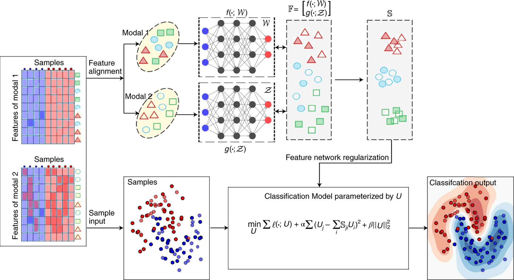
deepManReg inputs multi-modal datasets, e.g., Modal 1 (left top) and Modal 2 (left bottom), across the same set of samples. In Phase 1 (top flow), deepManReg aligns all features (the rows) across modalities by deep manifold alignment. In particular, it uses coupled deep neural networks $f\left(\cdot ;\mathcal{W}\right)$ and $g\left(\cdot ;\mathcal{Z}\right)$, parameterized with $\mathcal{W}$ and $\mathcal{Z}$ to project the features onto a common latent manifold space $\mathbb{F}$. The similarity matrix $\mathbb{S}$ of features on the latent space is then calculated, encoding the similarity of nonlinear manifolds among all pairs of both cross-modal and within-modal features. In Phase 2 (bottom flow), deepManReg inputs all the samples (the columns of the input data) into a regularized classification model, parameterized by U. The similarity matrix of features on the latent manifold space $\mathbb{S}$ in Phase 1 is used to regularize this classification model (i.e., via feature graph regularization), imposing similar features to have similar weights, when training. Finally, deepManReg outputs a regularized classification (i.e., deep manifold-regularized) for improving phenotype prediction and prioritizing cross-modal features for the phenotypes.

2. Results

Using our recent theoretic framework for multiview learning [6], deepManReg inputs multi-modal data of samples, aligns multi-modal features and predicts the samples’ phenotypes. There are two major phases in deepManReg: (Phase 1) aligning multi-modal features by deep-neural-network based manifold alignment (deep manifold alignment) for identifying nonlinear, cross-modal feature relationships on a common latent space, and (Phase 2) predicting the phenotypes of the samples from both modalities using the classification regularized by cross-modal feature relationships. Figure 1 illustrates these two phases of deepManReg workflow.

2.1. Classifying digits from multiple-features dataset

We first tested deepManReg by a multiple features (mfeat) dataset [11], which contains 2000 images of the handwritten digits 0–9 (i.e., 10 classes). In our experiment, two types of features, 216 profile correlations and 76 Fourier coefficients, which are considered as two modalities, are used to represent images. We applied deepManReg and compared with three other alignment methods, linear manifold alignment (LMA) [13], canonical correlation analysis (CCA) [14], and MATCHER [15], to the mfeat data.

Basically, CCA is a way of projecting the two data views on a common space that maximizes the correlation between them; linear manifold alignment is a manifold alignment method using linear operators for projection instead of using neural nets as in deepManReg for non-linear projection; MATCHER is a method for integrative analysis of single-cell measurements, aligning 1D pseudotime trajectories across different modalities (i.e., scRNA-seq and single-cell methylome in case of the original paper). The core of MATCHER is also manifold alignment, but not parameterized and thus not able to be generalized for new instances as in deepManReg.

In Phase 1, we did two separate experiments. The first one was for visualizing alignment performances only, in which the features from two modalities are projected onto a 2-dimensional (2D) space. Specifically, we defined two deep neural networks (DNNs) for cross-modal feature alignment in deepManReg with the same architecture with 2 hidden layers (500/100 hidden units) and 2 output-units. As shown in Figure 2, deepManReg outperforms CCA and LMA to align cross-modal features: the sums of pairwise distances on the latent space are 86.0, 165.8, and 56.9 for CCA, LMA, and deepManReg, respectively. We defined the partial correspondence between the two modalities as an all-ones matrix with size 76×216. As such, we obtained a similarity matrix with size 292×292.

Figure 2: Multi-modal feature alignment of handwritten digits.

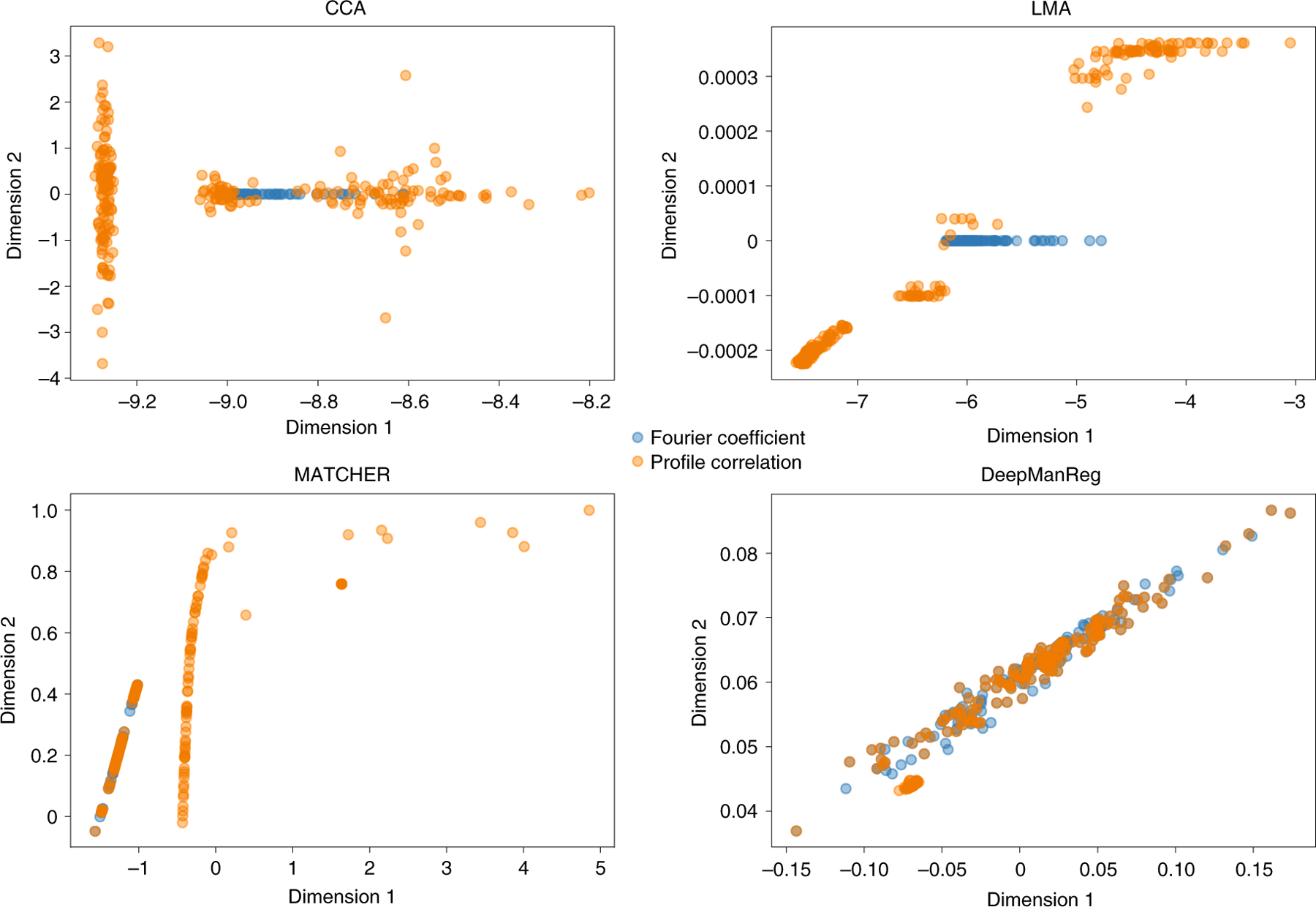
Two modalities, Fourier coefficient (Blue) and profile correlation (Orange), are aligned on a 2D common space. Each dot is a digit represented by either Fourier coefficient or profile correlation. The total sum of pairwise Euclidean distances between the features of two modalities on the latent space are 86.0, 165.8, 226 and 56.9 for CCA, Linear Manifold Alignment (LMA), MATCHER and deepManReg respectively.

In Phase 2, we also used a deep neural network model for classification with two hidden layers (200/50 hidden units) and regularize the model with the similarity matrix found in Phase 1, i.e., feature graph regularization. We did a multiple train-test splits, randomly splitting all samples into the training/testing sets with a stratified ratio of 80/20 10 times. As above, we also used other alignment methods to find the cross-modal feature graphs and regularize the classifications. Further, we directly input the raw data to the classification to get the result without using feature graph regularization. Figures 3A, 3B and Supplementary Figure 1 show that deepManReg outperforms the other methods by using cross-modal feature graph from its aligned latent space to regularize classification. To compare the classification accuracy across different methods, we used one-sided Kolmogorov-Smirnov test (k.s. test) to see if deepManReg’s accuracy is significantly higher than other methods. The null hypothesis in the one-sided k.s. test is that the accuracy distributions of deepManReg and another method are not different with the alternative hypothesis that they are different (deepManReg is higher). The k.s. test p-values are adjusted by Bonferroni correction. We found that the accuracy of deepManReg for the testing sets to classify digits is significantly higher than LMA (Kolmogorov–Smirnov (k.s.) test statistic = 0.7, p< 1e-2), MATCHER (k.s. test = 1.0 p< 2e-3), CCA (k.s. test = 0.7, p< 2e-3), and the classification without any regularization (k.s. test = 1.0, p< 1.08e-05). Also, its average accuracy, 80.3% is higher than the random guess baseline of 10% (ten labels), LMA (75.3% mean accuracy), CCA (72.8% mean accuracy), MATCHER (74.3% mean accuracy) and the average accuracy of the classification without regularization (10.0% mean accuracy). Moreover, as shown in Figure 3C, deepManReg also achieves relatively high Area under the ROC Curve (AUC) values (i.e, above 0.9) for classifying ten digits 0–9.

Figure 3: Regularized classification results for the mfeat digits dataset.

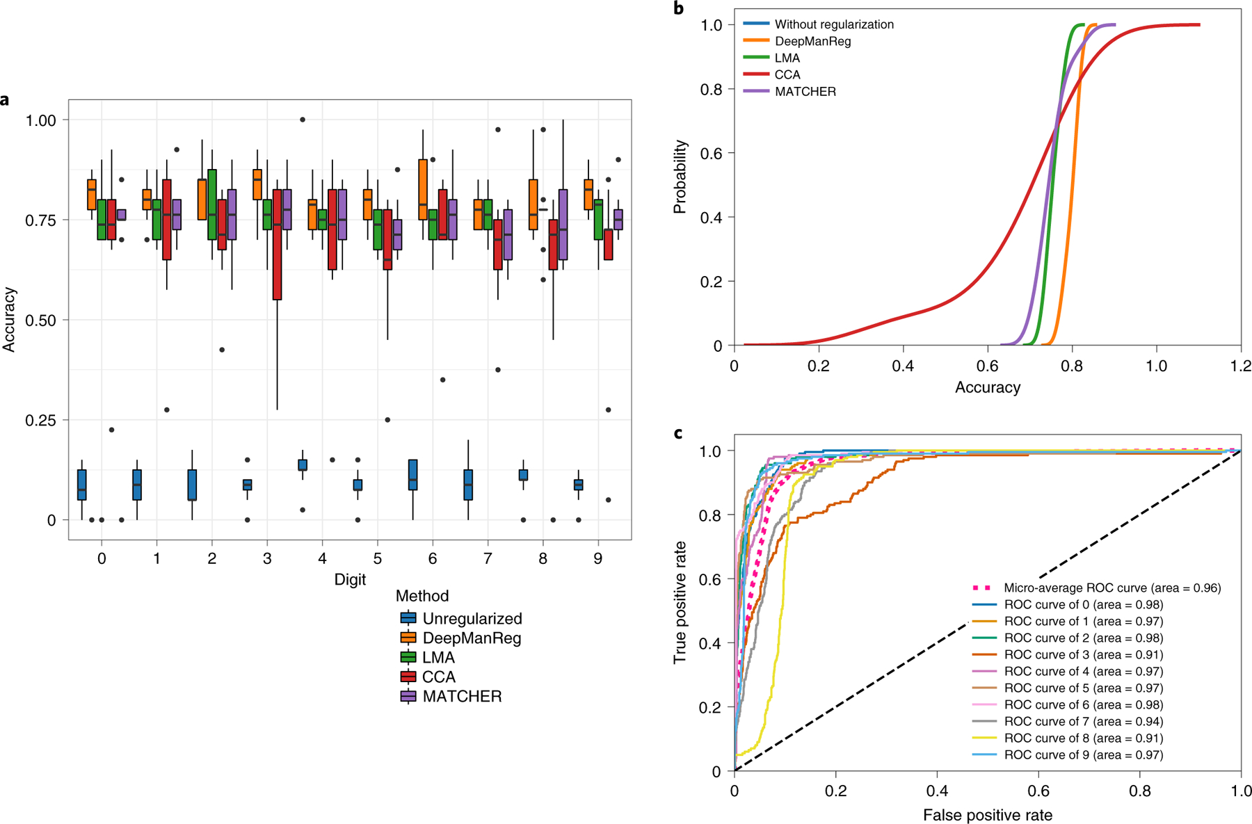
(A) Boxplot and (B) Cumulative distributions of testing accuracies for classifying digits by deepManReg (Orange) vs. the neural network classification without any regularization (Blue), by Linear Manifold Alignment (Green), CCA (Red), and MATCHER (Purple). The box extends from the lower to upper quartile values of the data (i.e., test accuracies of 10 experiments), with a line at the median. (C) Receiver operating characteristic (ROC) curves for classifying digits by deepManReg. x-axis: False Positive Rate, y-axis: True Positive Rate.

2.2. Reconstructing gene regulatory networks by simulation data

We also applied deepManReg on simulated multi-omics data [16] to show that the aligned feature graph by deepManReg can reconstruct gene regulatory networks. The simulated data is generated by dyngen [16], a multimodal simulator. It first defines a model gene regulatory network and then generates multi-omics data of genes by a set of reactions on the network, such as various molecular abundances (i.e., pre-mRNA, mRNA, protein) at multiple time points. We tested deepManReg and other alignment methods (e.g., CCA, LMA, MATCHER) using two modalities—namely, mRNA and protein abundances—driven by the example model data of dyngen consisting of 5 genes and their corresponding products in a closed-loop controlling feedback. We used the same hyperparameters from our two other applications (mfeat and Patch-set data), e.g., two hidden layers (500/100 hidden units) for deepManReg and default parameters for other methods. Specifically, we aligned two modalities, mRNA and protein abundances, of the network model, consisting of 5 genes (i.e., A, B, C, D, E) and their (activate or repress) relationships. After alignment (i.e., projecting two modalities onto the common manifold), we used kNN graphs (k=2) to reconstruct the network from projected data. As shown in Supplementary Figure 2, the evaluation results show that deepManReg outperforms other methods for reconstructing the model gene regulatory network that generates simulation data. To evaluate the differences between original network and reconstructed networks, we used the following score (which is similar to the manifold alignment formula) as evaluation metric: S = |X′ − Original| + |Y′ − Original| + |X′ − Y′ |, where X′ and Y′are the adjacency matrices of networks reconstructed by mRNA abundance and protein abundance (i.e., Modalities 1 and 2) respectively, and Original is the original model network adjacency matrix. The two first terms show the degree of matching between the reconstructed networks (from two modalities) and the original network, and the third term evaluates the alignment of reconstructed networks by two modalities. Thus, the lower score, the better reconstruction. We found that deepManReg has a lower score (i.e., 16) than all other methods. This suggests that the capability of deepManReg for reconstructing gene regulatory networks via its aligning multi-omits features.

2.3. Classifying cellular phenotypes from multi-modal data

Recent Patch-seq technique measures multi-modal characteristics of single cells such as transcriptomics, electrophysiology and morphology [17]. For example, the Brain Initiative project has generated multimodal data of neuronal cells in the human and mouse brains [12]. Using those single-cell multi-modal data, ones have identified many cell types corresponding to various cellular phenotypes. Here, we applied deepManReg to recent Patch-seq data for the mouse visual cortex from Allen Brain Atlas for predicting neuronal phenotypes, including cell layers and transcriptomic types. Specifically, this dataset includes the transcriptomic, and electrophysiological data of 4435 neuronal cells (GABAergic cortical neurons) in the mouse visual cortex [12]. For cellular phenotypes for our prediction, we included six transcriptomically defined neuronal cell types (t-types), based on primarily expressed genes: Vip-type, Sst-type, Sncg-type, Serpinf1-type, Pvalb-type, and Lamp5-type, and five cell layers revealing the locations of cells on the visual cortex: L1, L2/3, L4, L5, and L6.

2.3.1. Single cell multi-modal dataset and data processing

The electrophysiological data includes the responses of three stimuli: short (3 ms) current pulses, long (1 s) current steps, and slow (25 pA/s) current ramp current injections. We extracted 47 electrophysiological features (e-features) on stimuli and responses, identified by Allen Software Development Kit (Allen SDK) and IPFX Python package [18]. We then filtered the e-features with many missing values, extracted the cells from t-types and layers as above, and finally selected 41 e-features for 3654 neuronal cells. The transcriptomic data quantifies gene expression levels of the neuronal cells on the genome wide. We extracted the 1000 genes that have the highest expression variations among the 3654 cells. Then, we input the log-transformed gene expression and e-features of those cells as input multi-modal data into deepManReg for predicting cellular phenotypes, i.e., X is 1000 genes by 3654 cells and Y is 41 e-features by 3654 cells. As shown in Figure 4, the latent space from deep manifold alignment (Phase 1) reveals that many genes and e-features have strong nonlinear relationships (via aligned cross-modal manifolds) (Supplementary Figure 3).

Figure 4: The network showing the relationships across two modalities—genes and electrophysiology.

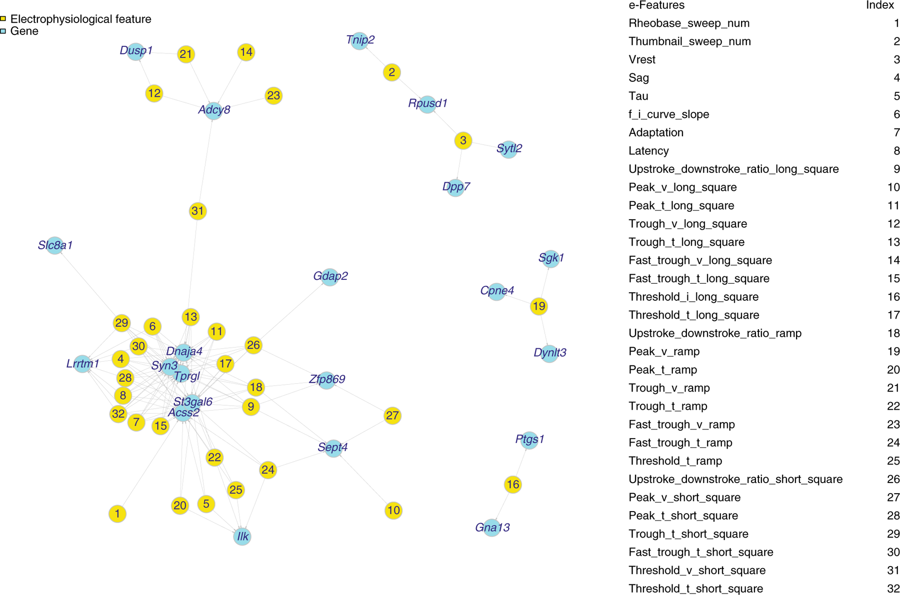
The genes and electrophysiological features (e-features) of neuronal cells in the mouse visual cortex having small Euclidean distances on the aligned latent space by deepManReg Phase 1, i.e., deep manifold alignment. Cyan: genes. Yellow: e-features. Nodes are connected by Similarity = 1/(1+Euclidean distance) > 0.997 on 3D aligned space.

2.3.2. Aligning genes with electrophysiology for classification

We first applied the deep manifold alignment from deepManReg (Phase 1) into the multi-modal feature set of the mouse visual cortex (1041 in total). To find the common latent space, we constructed two deep neural networks with the same architecture of 2 hidden layers (512/64 hidden units) and reproduced a 3-dimensional latent space for similarity measurement. The partial correspondence matrix W is a 1041×1041 matrix defined by a combination of correlation matrix between two feature modalities (1000×41 on the top left, 41×1000 on the bottom right) and the kNN (k = 5) graph within each modality (1000×1000 in the top right, 41×41 on the bottom left). As a comparison, we applied linear manifold alignment (LMA), canonical-correlation analysis (CCA) with the correspondence matrix constructed the same way, and MATCHER [15] to get three other latent spaces, and then constructed a similarity matrix in the latent space for regularization in Phase 2. We also directly applied the raw data of the features to the classification, i.e., without regularization. In addition, deepManReg ran faster than other methods for alignment, e.g., with the running times by a laptop with CPU i5–8250U: CCA (725.96 seconds), Manifold Alignment (663.43 seconds), MATCHER (150.94 seconds), and deepManReg (90.10 seconds). If GPU GTX 1060Ti was used for deep learning, deepManReg alignment took 57.90 seconds.

After multi-modal feature alignment, we applied deepManReg to use the distances of genes and e-features on the latent space as a ”feature graph” to regularize another deep neural network model to classify the cellular phenotypes such as cortical layers of cells in the brain, which is achieved by adding a regularization term into the neural network model (Methods). In particular, the regularization matrix is a 1000×41 matrix by assigning the observations over 50% percentile in matrix 1/(1+distance) to be 1 and others to be 0. The neural network for classification has the input layer consisting of 1041 nodes (1000 genes + 41 e-features), two hidden layers (100/50 hidden units) and the final output layer with the same number of units as phenotypes along with a Softmax operation. For instance, for classifying cell layers, the five output units represent L1, L2/3, L4, L5, and L6. We randomly split all cells into the training/testing sets with a stratified ratio of 80/20 and obtained 500 sets. For each training set, we oversampled the cells from each label to be 941 cells and thus balance sample sizes across labels (e.g., L1: 262 cells; L2/3 1097 cells; L4: 385 cells; L5: 1176 cells; L6:734 cells) [19]. As shown in Figures 5A, 5B, and Supplementary Figure 4, the prediction accuracy of deepManReg for the testing sets to classify cell layers is significantly higher than other methods (k.s. test p-values < Bonferroni corrected cutoff 0.05/6=0.0083): LMA (k.s. test statistic = 0.95, p< 2.8003221e-50), CCA (k.s. test statistic = 0.80, p< 1.7820141e-32), MATCHER (k.s. test statistic = 0.72, p< 1.3383191e-25), and the classification without any regularization (k.s. test statistic = 0.89, p< 4.2826771e-42). Besides, deepManReg outperforms the neural network classifications using single modality only, i.e., e-features only (k.s. test statistic = 0.89, p < 4.2826771e-42) and gene expression only (k.s. test statistic = 0.98, p < 2.1977161e-55). Also, its average accuracy, 51.4% (with a 95% confidence interval [47.9%, 54.8%]) is higher than the random guess baseline of 20% (five labels), LMA (43.0% mean accuracy, [32.2%, 49.6%] confidence interval), CCA (46.2% mean accuracy, [40.1%, 51.3%] confidence interval), MATCHER (46.5% mean accuracy, [40.9%, 52.8%] confidence interval), e-features only (30.1% mean accuracy, [7.1%, 51.8%] confidence interval), gene expression only (44.0% mean accuracy, [40.4%, 47.4%] confidence interval), and the average accuracy of the classification without regularization (30.6% mean accuracy, [7.1%, 51.6%] confidence interval). Moreover, as shown in Figure 5C, deepManReg also achieves relatively high AUC values of 0.96, 0.86, 0.84, 0.79, and 0.91 for the five layers L1, L2/3, L4, L5, and L6, respectively. In addition to predicting cell types, we also found that deepManReg outperforms other methods for predicting t-types, i.e., average accuracy 90% ([87.0%, 93.4%] confidence interval) for deepManReg vs. 35.0% ([3.2%, 76.8%] confidence interval) for LMA vs. 71.6% ([48.2%, 86.4%] confidence interval) for CCA vs. 71.1% ([50.6%, 89.1%] confidence interval) for MATCHER vs. 64.1% ([20.1%, 92.9%] confidence interval) for classification without regularization. These results show that the regularized classification by deepManReg’s alignment improves predicting cellular phenotypes from single cell multimodal data. This also suggests the contributions from the nonlinear manifold relationships of gene expression and electrophysiology to the cellular phenotypes.

Figure 5: Regularized classification results for single-cell multi-modal data in the mouse visual cortex.

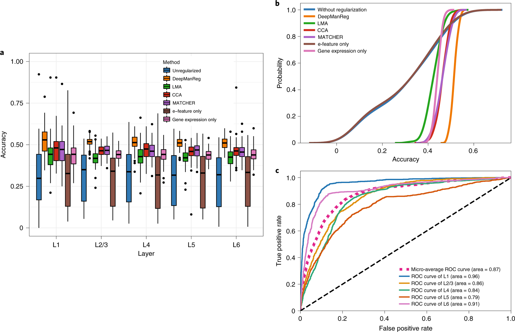
(A) Boxplots and (B) Cumulative distributions of testing accuracies for classifying cell layers in the mouse visual cortex by deepManReg (Orange) vs. neural network classification without any regularization using both modalities (Blue), Electrophysiological features (E-feature) only (Brown), and gene expression only (Pink) by Linear Manifold Alignment (Green), CCA (Red), and MATCHER (Purple). The box extends from the lower to upper quartile values of the data (i.e., test accuracies of 100 experiments), with a line at the median. (C) Receiver operating characteristic (ROC) curves for classifying cell layers in the mouse visual cortex by deepManReg. Cell layers include Blue: L1, Yellow: L2/3, Green: L4, Orange: L5 and Purple: L6. x-axis: False Positive Rate, y-axis: True Positive Rate.

2.3.3. Prioritizing multi-modal features for cellular phenotypes

After training a deepManReg model, we further used a derivative-based method called integrated gradient [20] to prioritize genes and e-features for each phenotype (e.g., cell layers in Supplementary Data 1). Specifically, we calculated the gradient of the model’s prediction for each e-feature and/or gene to quantify the changes of the output response values (e.g., cell layers) by a small change of input gene expression and e-feature values [21]. We used the recent Python package, Captum [22] to implement the integrated gradient method and calculate the importance scores of each gene/e-feature for output labels (i.e., cellular phenotypes). We then ranked the genes and e-features by the scores and prioritized top ones for each phenotype. For instance, we summarized top prioritized genes and e-features for each cell layer in Supplementary Data 1. To evaluate the prioritization of cross-modal features, we calculated their Spearman correlation coefficients across cells. As shown on Supplementary Figure 5, the prioritized genes and e-features for each layer have higher Spearman correlations across the layer’s cells than the rest of the cells (one-sided t-test p ¡ 0.0001 for Layer 1, 0.0004 for Layer 2/3, 0.0001 for Layer 4, 0.11 for Layer 5 and 0.13 for Layer 6). This suggests that our deepManReg identifies such cross-modal feature interactions for different cortical layers. However, Spearman correlation is a ranking based correlation, only providing descriptive measurements between genes and e-features. Thus, deepManReg is further able to uncover predictive cross-modal interactions for classifying cortical layers.

3. Discussion

Our deepManReg method learns multiple deep neural networks for different modalities and jointly trains them to align multi-modal features onto a common latent space. The distances of various features within and between modalities on the space represent their nonlinear relationships identified by cross-modal manifolds. The applications in the paper focus on classification, but the loss function of the regularized learning in deepManReg (Phase 2) can work generally for regression as well, i.e., to predict continuous phenotypes. Specifically, the loss function in Phase 2 of deepManReg is in general form where the label o_k can take discrete or continuous values. If o_k is continuous and loss l(·, U ) is a square loss, the learning problem becomes a regression problem.

Although we demonstrated that deepManReg works for two particular datasets, deepManReg can be generalized to any multi-modal data such as additional single cell omics (scATAC-seq, scHi-C, etc) (Methods). Also, the architectures of its deep neural networks for manifold alignment can be designed specific for each modality. For example, if two modalities are genomics and images, the neural network for aligning images can be changed to a convolutional neural network. Also, one can model those neural networks by recent graph neural networks [23], aiming to not only align multi-modal features but also underlying biological networks in the modalities.

deepManReg solves the trade-off between nonlinear and parametric manifold alignment (by utilizing the nonlinearity and parametric of neural architecture which is trained by a Riemannian optimization procedure). Specifically, deepManReg solved the non-linear projections (from multiple datasets) by gradient descent on a Stiefel manifold. One significant advantage of deepManReg is that it is a parameterized method: using two deep neural nets as projection functions and learning the networks’ parameters by backpropagating the Riemannian gradient of the gradient descent procedure so that it can generalize to new instances. Solving non-linear dimension reduction by gradient descents on Stiefel manifold has been researched extensively [24] and well implemented [25]. To our knowledge, however, this is the first time a parameterized non-linear method has been proposed so the projection can be generalized for unseen data. Although generalized Stiefel manifolds have been developed thoroughly [26], our solution showed that, calculating the gradient on the (plain) Stiefel manifold is more efficient for two reasons: (1) the matrix multiplication is simpler because we only need to calculate FF^T, not FLF^T as in generalized Stiefel manifold, and (2) we have the closed form solution [24] for the projection onto the (plain) Stiefel manifold that is of the essence since this is the last layer of the model and needs to be differentiable.

Furthermore, deepManReg works as both representation learning and regularized classification. Since dimensionality reduction is the essential characteristic of manifold alignment, deepManReg is scalable for various input feature sizes and thus able to perform the transcriptome-wide analysis such as inputting all possible genes. We experimented with different numbers of highly variable genes and found that the average accuracies for classifying five major cortical layers do not change too much: 53.1% for 500 genes, 51.4% for 1000 genes, and 49.1% for 2000 genes. However, training deepManReg requires a non-trivial hyperparameter optimization since training two deep neural networks simultaneously includes a large combination of parameters. Another potential issue for aligning such large datasets in deepManReg which may be computational intensive is the large joint Laplacian matrix (Supplementary Algorithm). Thus, how to reduce the computational burden in deepManReg will be a key future improvement. For example, we may use the Nystrom method [27] to approximate the Laplacian matrix for making deepManReg more scalable and computationally efficient.

It is also worth noting that there are differences between deepManReg and other geometric-based learning methods: (a) structured-output learning methods, such as graph neural networks can only learn the structures or relationships among samples [23]; (b) graph-regularized learning methods (mostly based on Laplacian graphs [28, 29, 30], spectral graph convolutions [31]) use the relationships of features to regularize the learning model but aim to penalize each network edge, rather than each feature itself [10]. Moreover, manifold learning has been used to align single cell multi-omics data, aiming to find the correspondence across single cell multi-omics, such as in MATCHER [15] and MMD-MA [32]. While MATCHER works mainly on a bi-modal data (i.e., DNA methylation and gene expression), MMD-MA can work on multiple modals and does not require the correspondence among modals by means of a maximum mean discrepancy (MMD) term. Thus, deepManReg can be extended in a similar way in which the correspondence matrix is not given but learned using manifold warping [33] or local geometry matching [13]. Furthermore, deepManReg can also be generalized to integrate more than two modalities by concatenating input data and similarity matrices, aiming to improve phenotype prediction from multi-modal data and prioritize cross-modal features for phenotypes.

4. Methods

Using our recent theoretic framework for multiview learning [6], deepManReg inputs multi-modal data of samples, aligns multi-modal features and predicts the samples’ phenotypes. For instance, two modalities of a set of p samples can be modeled as $T={\left\{z_k,t_k,o_k\right\}}_{k=1}^p$ with $z_k\in {ℝ}^n$ being the kth sample of Modal 1 and $t_k\in {ℝ}^m$ being the kth sample of Modal 2, and associated phenotypes for both modalities (i.e., labels) $o_k\in \mathcal{O}$. Also, Modal 1 and Modal 2 have n and m features, respectively. The features of Modal 1 and Modal 2 are modeled as $X={\left\{x_i\right\}}_{i=1}^n$ and $Y={\left\{y_j\right\}}_{j=1}^m$ respectively, where $x_i\in {ℝ}^p$ is the ith feature of Modal 1 and $y_j\in {ℝ}^p$ is the jth feature of Modal 2. In matrix notation, z_k and x_i are respectively columns and rows of the same matrix, representing Modal 1 data. Similarly, t_k and y_j are of the matrix representing Modal 2 data. There are two major phases in deepManReg: (Phase 1) aligning multi-modal features, i.e. ${\left\{x_i\right\}}_{i=1}^n$ and ${\left\{y_j\right\}}_{j=1}^m$, by deep-neural-network based manifold alignment (deep manifold alignment) for identifying nonlinear, cross-modal feature relationships on a common latent space, and (Phase 2) predicting the phenotypes ${\left\{o_k\right\}}_{k=1}^p$ of the samples from both modalities, i.e., ${\left\{z_k,t_k\right\}}_{k=1}^p$, using the classification regularized by cross-modal feature relationships.

4.1. Phase 1: Deep manifold alignment of multi-modal features

4.1.1. Parametric nonlinear alignment via manifolds

Manifold alignment is a class of techniques for learning representations of multiple data views, such that the presentation of each view is the most predictive of, and, at the same time, the most predictable by, the representation of other views. It can also be considered as a generalization of canonical correlation analysis (CCA) [14] whereas the intrinsic geometry of data views are preserved and/or the projections are nonlinear [6].

Manifold alignment has been applied to identify linear (feature-level) projections, or nonlinear (instance-level) embeddings of multi-modal data. While the instance-level version generally aligns and matches different data-views with high accuracy, it cannot be generalized for new instances since the new coordinates in the common latent space are learned directly, not via parameterized projections. The feature-level version is generalizable, allowing new instances to be easily embedded into the learned latent space via parameterized yet linear projections. These properties are crucial for transferring knowledge across modalities. Thus, deepManReg simultaneously learns different nonlinear mappings for different data modalities for discovering cross-modal manifolds and aligns them onto a common latent space. This idea combines appealing properties of both feature-level and instance-level projections for achieving accurate alignment and generalization. Furthermore, traditional solutions for manifold alignment rely on the eigendecompostion that is typically computationally intensive. To improve this, we utilize the stochastic gradient descent (SGD) and backpropagation techniques for speeding up training in deepManReg.

Particularly, deepManReg first calculates the similarities in terms of nonlinear manifolds among all possible features across modalities. To this end, deepManReg conducts a deep manifold alignment between all features so that the features are aligned onto a common latent space. The distances of the features on the latent space thus reveal such similarities of the features in terms of nonlinear manifold structures, suggesting nonlinear, cross-modal feature relationships. Mathematically, given two modal datasets, $X={\left\{x_i\right\}}_{i=1}^n$ and $Y={\left\{y_j\right\}}_{j=1}^m$ where X are the features of Modal 1 and Y are the features of Modal 2, and the partial correspondences between the instances in X and Y, encoded by the matrix $W_{\left(X,Y\right)}\in {ℝ}^{n\times m}$, we want to learn the two mappings f (.) and g(.) that map x_i and y_j to $f\left(x_i\right)\in {ℝ}^d$ and $g\left(y_j\right)\in {ℝ}^d$, respectively onto the latent space with dimension d ≪ p that preserves the local geometry of X, Y and also matches cross-modal features from the correspondence. The correspondence matrix W_{(X,Y )} could be defined as $W\left(i,j\right)=\{\begin{array}{ll}1\hfill & \text{if}\hspace{0.17em}{X}_i\hspace{0.17em}\text{and}\hspace{0.17em}{Y}_j\hspace{0.17em}\text{are}\hspace{0.17em}\text{correspondent}\hspace{0.17em}\text{to}\hspace{0.17em}\text{each}\hspace{0.17em}\text{other}\hfill \\ 0\hfill & \hspace{1em}\hspace{1em}\hspace{1em}\hspace{1em}\hspace{1em}\hspace{1em}\hspace{0.17em}\hspace{0.17em}\hspace{0.17em}\hspace{0.17em}\text{otherwise}\hfill \end{array}$ and thus need otherwise not be symmetric.

Further, the instance x_i is correspondent to the instance y_j if and only if f (x_i) = g(y_j). Besides, any prior correspondence information between the features from different modalities can be used as partial information to initially build the corresponding matrix W_{(X,Y )}. After mappings, $f\left(X\right)\in {ℝ}^{n\times d}$ and $g\left(Y\right)\in {ℝ}^{m\times d}$ represents the new coordinates of the features of Modal 1 and 2 on the latent space with the dimension d, respectively. That said, the concatenation of the new coordinates $\mathbb{F}=\left[\begin{array}{l}f\left(X\right)\\ g\left(Y\right)\end{array}\right]$ the unified representation of the features from X and Y on the common latent space.

Then, according to [34], the loss function for manifold alignment can be formed as the Laplacian eigenmaps [35] using the joint Laplacian and the joint adjacency matrix of the two datasets:

$$\ell \left(\mathbb{F}\right)=\sum _{i,j}{\Vert \mathbb{F}\left(i,\cdot \right)-\mathbb{F}\left(j,\cdot \right)\Vert }^{2}W\left(i,j\right),$$

where the sum is taken over all pairs of instances from both datasets, $\mathbb{F}$ is the unified representation of both datasets, and $W=\left[\begin{array}{cc}{W}_X& W_{\left(X,Y\right)}\\ W_{\left(X,Y\right)}^T& W_Y\end{array}\right]$ is the joint similarity matrix (W_x and W_y are similarity matrices within each dataset X and Y )

Using the facts that ${\Vert M\left(i,\cdot \right)\Vert }^2={\sum }_{k}M{\left(i,k\right)}^2$ and that the Laplacian is a quadratic difference operator, the above equation can be transformed into:

$$\ell \left(\mathbb{F}\right)=\sum _{i,j}\sum _k{\left(\mathbb{F}\left(i,k\right)-\mathbb{F}\left(j,k\right)\right)}^{2}W\left(i,j\right)$$ (1)

$$=tr\left({\mathbb{F}}^{T}L\mathbb{F}\right),$$ (2)

where L = D − W (D is the diagonal matrix of W ) is the joint Laplacian [34] of both datasets.

For this loss function to work properly, i.e., avoiding a trivial solution of mapping all instances to zero, we need an additional constraint:

$${\mathbb{F}}^{T}D\mathbb{F}=\mathbb{I},$$

where D is the diagonal matrix of W and $\mathbb{I}$ is the d × d identity matrix.

Finally, we solve the following optimization problem for manifold alignment, i.e., to find the optimal mapping functions f (.) and g(.):

$$\underset{f,g}{\min }tr\left({\mathbb{F}}^{T}L\mathbb{F}\right)$$

$$\text{s}.\text{t}.{\mathbb{F}}^{T}D\mathbb{F}=\mathbb{I}.$$

Normally, this optimization can be solved by eigendecomposition [4], which however is computationally intensive. Moreover, solving generalized eigenvector problem gives us merely the new coordinates of the latent manifold (i.e., Xʹ = f(X), Yʹ = g(Y )), not the closed form of mappings themselves (i.e., f (·) and g(·)), and thus is incapable of generalizing for new instances. To solve this, we parameterized the mappings f (·) and g(·) by using coupled deep neural networks (Section 2.1.2) and finally form the optimization problem as below:

$$\underset{f,g}{\min }tr\left({\widehat{\mathbb{F}}}^T\widehat{L}\widehat{\mathbb{F}}\right)$$

$$\text{s}.\text{t}.{\widehat{\mathbb{F}}}^T\widehat{\mathbb{F}}=\mathbb{I}$$

if we set $\widehat{\mathbb{F}}=\mathbb{F}{D}^{1/2}$ and $\widehat{L}=D^{-1/2}L{D}^{-1/2}$.

This is actually an optimization problem on the Stiefel manifold, where the feasible set of the orthogonality constraints $S_{n,p}:=\left\{X\in {ℝ}^{n\times p}:X^{T}X=\mathbb{I}\right\}$ is referred to as the Stiefel manifold [36].

4.1.2. Nonlinear manifold co-embedding by deep neural networks

As above, we model the relationships between the observable data x_i, y_j and its latent representation f (x_i), g(y_j ) using two nonlinear mappings $f\left(x_i;\mathcal{W}\right)$, $g\left(y_j;\mathcal{Z}\right)$ where $f\left(\cdot ;\mathcal{W}\right)$, $g\left(\cdot ;\mathcal{Z}\right)$ denote the mapping functions and $\mathcal{W}$, $\mathcal{Z}$ denote the set of the function parameters. In deepManReg, we employ the deep neural networks (DNNs) to model our mapping functions, since DNNs have the ability of approximating any continuous mapping using a reasonable number of parameters. Note that, of the two DNNs, the numbers of input nodes are unnecessary to be the same, but the numbers of output nodes (i.e., latent representations of two modal features) have to be exactly the same for allowing having a common latent space. Precisely, if $X\in {ℝ}^{n\times p}$ is a matrix of data row vectors $x_i\in {ℝ}^p$, the number of input nodes for the first network $f\left(\cdot ;\mathcal{W}\right)$ is p, and if $Y\in {ℝ}^{m\times q}$ is a matrix of data row vectors $y_j\in {ℝ}^q$, the number of input features for the second network $g\left(\cdot ;\mathcal{Z}\right)$ is q. The number of output represented features of both DNNs is d, the dimension of the common latent manifold space.

4.1.3. Training neural networks by Stiefel manifolds for alignment

There exist two key issues for generalizing backpropagation to train our DNNs for deep manifold alignment. The first one is preserving the manifold constraint in the output layer. As we force the outputs to be on Stiefel manifolds, merely using the forward propagation in the normal DNN is not guaranteed to yield valid orthogonal outputs. Second, while the gradient of loss function with respect to output layer, i.e., $\widehat{\mathbb{F}}$, can be calculated easily, computing those with hidden layers, i.e. $\mathcal{W}$, $\mathcal{Z}$ has not been well-solved by the traditional backpropagation.

To solve the first issue of preserving the constraint, we construct the last layer by projecting the output of the preceding layer $\left[\begin{array}{c}f\left(X\right)\\ g\left(Y\right)\end{array}\right]$ onto the Stiefel manifold S_m+n,d. Specifically, we use the classical projection operator π(·) which is defined as:

$$\widehat{\mathbb{F}}=\pi \circ \left[\begin{array}{c}f\left(X\right)\\ g\left(Y\right)\end{array}\right]=\underset{Z\in S_{m+n,d}}{\arg \min }{\Vert \left[\begin{array}{c}f\left(X\right)\\ g\left(Y\right)\end{array}\right]-Z\Vert }_F^2.$$

It is known that the solution of this problem is given by

$$\widehat{\mathbb{F}}=U{\mathbb{I}}_{m+n,d}{V}^T,$$

where $\left[\begin{array}{c}f\left(X\right)\\ g\left(Y\right)\end{array}\right]=U\Sigma V^T$ is the SVD decompostion of $\left[\begin{array}{c}f\left(X\right)\\ g\left(Y\right)\end{array}\right]$. Thus, $\widehat{\mathbb{F}}$ now is an orthogonal output, i.e. ${\widehat{\mathbb{F}}}^{T}D\widehat{\mathbb{F}}=\mathbb{I}$.

As for the second issue, we have developed a new way of updating the weights $\mathcal{W}$, $\mathcal{Z}$ by exploiting an SGD setting on the Stiefel manifolds. The steepest descent direction for the corresponding loss function $\ell \left(\widehat{\mathbb{F}}\right)$ with respect to $\widehat{\mathbb{F}}$ on the Stiefel manifold is the Riemannian gradient ${\tilde{\nabla }}_{\widehat{\mathbb{F}}}l$. To obtain it, the Euclidean gradient ${\nabla }_{\widehat{\mathbb{F}}}\ell =\frac{\partial tr\left({\widehat{\mathbb{F}}}^T\widehat{L}\widehat{\mathbb{F}}\right)}{\partial \widehat{\mathbb{F}}}=\widehat{L}\widehat{\mathbb{F}}+{\widehat{L}}^{\top }\widehat{\mathbb{F}}$ is projected onto the tangent space $T_{\widehat{\mathbb{F}}}\left(S_{m+n,d}\right)$ of Stiefel manifold S_m+n,d. The projection is defined as

$$\begin{array}{l}{\tilde{\nabla }}_{\widehat{\mathbb{F}}}\ell =\pi \left({\nabla }_{\widehat{\mathbb{F}}}\ell \right)=\underset{X\in T_{\widehat{\mathbb{F}}}\left(S_{m+n,d}\right)}{\arg \min }{\Vert {\nabla }_{\widehat{\mathbb{F}}}\ell -X\Vert }_F^2\\ \hspace{0.17em}\hspace{0.17em}\hspace{0.17em}\hspace{0.17em}\hspace{0.17em}\hspace{0.17em}\hspace{0.17em}\hspace{0.17em}\hspace{0.17em}\hspace{0.17em}\hspace{0.17em}\hspace{0.17em}\hspace{0.17em}\hspace{0.17em}\hspace{0.17em}\hspace{0.17em}\hspace{0.17em}\hspace{0.17em}\hspace{0.17em}\hspace{0.17em}\hspace{0.17em}\hspace{0.17em}\hspace{0.17em}\hspace{0.17em}\hspace{0.17em}\hspace{0.17em}\hspace{0.17em}\hspace{0.17em}\hspace{0.17em}\hspace{0.17em}\hspace{0.17em}\hspace{0.17em}=\widehat{\mathbb{F}}skew\left({\widehat{\mathbb{F}}}^T{\nabla }_{\widehat{\mathbb{F}}}\ell \right)+\left(I-\widehat{\mathbb{F}}{\widehat{\mathbb{F}}}^T\right){\nabla }_{\widehat{\mathbb{F}}}\ell ,\end{array}$$

where $skew\left({\widehat{\mathbb{F}}}^T{\nabla }_{\widehat{\mathbb{F}}}\ell \right)=\frac{1}{2}\left({\widehat{\mathbb{F}}}^T{\nabla }_{\widehat{\mathbb{F}}}\ell -{\left({\nabla }_{\widehat{\mathbb{F}}}\ell \right)}^T\widehat{\mathbb{F}}\right)$. The project of $\left[\begin{array}{c}f\left(X\right)\\ g\left(Y\right)\end{array}\right]$ onto the Stiefel manifold and the Euclidean gradient onto the tangent space of the Stiefel manifold are illustrated in Supplementary Figure 6.

Putting all together, we summarized our optimization for deep manifold alignment in Supplementary Algorithm, which can be readily implemented with the modern tools for automatic differentiation such as PyTorch [37].

4.2. Phase 2: Regularized classification by cross-modal feature relation-ships

After finding the common latent space from deep manifold alignment, we can now calculate the distance matrix $\mathbb{D}$ for each row pairs of matrix $\widehat{\mathbb{F}}$, and then similarity matrix $\mathbb{S}=\frac{1}{1+\mathbb{D}}$. The latter finally gives the similarities of all multi-modal features in terms of nonlinear manifold structures, systematically evaluating cross-modal feature relationships.

In Phase 2 of deepManReg, we want to improve phenotype prediction from multi-modal data using such cross-modal feature relationships. In particular, back to the training set $T={\left\{z_k,t_k,o_k\right\}}_{k=1}^p$, deepManReg learns a classifier paramaterized by a weight $U\in {ℝ}^{\left(m+n\right)\times d}$ by minimizing a loss function $\ell \left(z,t,o;U\right)$ over the training instances (z_k, t_k, o_k) [10]. U has m + n columns (total number of cross-modal features) and d rows (number of reduced dimensions on the aligned latent space). Now, with the similarity information of features, provided by matrix $\mathbb{S}$ from the previous step, we can use $\mathbb{S}$ as an adjacency matrix of a feature graph encoding the relationship between all pairs of features within and across modalities. The degree of each vertex in the feature graph has to be sum to one, ${\sum }_j{\mathbb{S}}_{ij}=1$, to avoid some features dominating the whole graph. Because similar features should have similar weights after training, we regularize each feature’s weight by the squared amount that it differs from the weighted average of its neighbors. Thus, the loss function for this feature-graph-regularized learning is given by [10]:

$$loss\left(U\right)=\sum _{k=1}^p\ell \left(z_k,t_k,o_k;U\right)+\alpha \sum _{j=1}^{n+m}{\left(U_j-\sum _i{\mathbb{S}}_{ji}{U}_i\right)}^2+\beta {\Vert U\Vert }_2^2.$$

The hyperparameters α and β are to balance between the feature graph regularization and the ridge regularization. Finally, the combined regularization can be rewritten as U^T MU where $M=\alpha {\left(I-\mathbb{S}\right)}^T\left(I-\mathbb{S}\right)+\beta I$. We also did an ablation study on the values of α and β and found that the larger α is, the higher prediction accuracy our model has (Supplementary Table 1). This implies that our feature-network regularized term contributes to improved classification more than the L2 term. The classification improvement by feature-network regularization was also observed in previous studies [10].

The classifiers can be general. In practice, here, we use a neural network as a classifier so the optimization problem above can be solved easily with gradient descent methods. Also, we can use other approaches for regularization such as the graph Laplacian [10]. The main difference between the Laplacian regularization and the feature graph regularization is that the former penalizes each edge (between two features) equally while the latter penalizes each feature (e.g., nodes) equally. The efficiency of the approaches depends on the problem domain.

4.3. Data Availability

The multiple-features (mfeat) dataset is available at [11]. The Patch-seq transcriptomics data and electrophysiological data are available at [12]. The simulated multi-omics data and gene regulatory network (i.e., the example model data of dyngen for 5 genes) are available at [16]. Source Data are available with this paper.

4.4. Code Availability

Code for deepManReg implementation and data analysis are available at https://github.com/daifengwanglab/deepManReg. An interactive version of the code base is provided in [38].

4.5. Statistics & Reproducibility

To compare the classification accuracy across different methods, we used one-sided Kolmogorov-Smirnov test (k.s. test) to see if deepManReg’s accuracy is significantly higher than other methods. The null hypothesis in the one-sided k.s. test is that the accuracy distributions of deepManReg and another method are not different with the alternative hypothesis that they are different (deepManReg is higher). The k.s. test p-values are adjusted by Bonferroni correction. No statistical method was used to predetermine sample size.

References

- 1.Larranaga Pedro, Calvo Borja, Santana Roberto, Bielza Concha, Galdiano Josu, Inza Inaki, Lozano José A, Armananzas Rubén, Santafé Guzman, Pérez Aritz, et al. Machine learning in bioinformatics. Briefings in bioinformatics, 7(1):86–112, 2006. [DOI] [PubMed] [Google Scholar]
- 2.Subramanian Indhupriya, Verma Srikant, Kumar Shiva, Jere Abhay, and Anamika Krishanpal. Multi-omics data integration, interpretation, and its application. Bioinformatics and biology insights, 14:1177932219899051, 2020. [DOI] [PMC free article] [PubMed] [Google Scholar]
- 3.Sima Chao, Attoor Sanju, Brag-Neto Ulisses, Lowey James, Suh Edward, and Dougherty Edward R. Impact of error estimation on feature selection. Pattern Recognition, 38(12):2472–2482, 2005. [Google Scholar]
- 4.Wang Chang and Mahadevan Sridhar. A general framework for manifold alignment. In AAAI fall symposium: manifold learning and its applications, pages 79–86, 2009.
- 5.Nguyen Nam D, Blaby Ian K, and Wang Daifeng. Maninetcluster: a novel manifold learning approach to reveal the functional links between gene networks. BMC genomics, 20(12):1–14, 2019. [DOI] [PMC free article] [PubMed] [Google Scholar]
- 6.Nguyen Nam D and Wang Daifeng. Multiview learning for understanding functional multiomics. PLoS computational biology, 16(4):e1007677, 2020. [DOI] [PMC free article] [PubMed] [Google Scholar]
- 7.Brorson Ina S, Eriksson Anna, Leikfoss Ingvild S, Celius Elisabeth G, Berg-Hansen Pål, Barcellos Lisa F, Berge Tone, Harbo Hanne F, and Bos Steffan D. No differential gene expression for cd4+ t cells of ms patients and healthy controls. Multiple Sclerosis Journal–Experimental, Translational and Clinical, 5(2):2055217319856903, 2019. [DOI] [PMC free article] [PubMed] [Google Scholar]
- 8.Ng Andrew Y. Feature selection, l 1 vs. l 2 regularization, and rotational invariance. In Proceedings of the twenty-first international conference on Machine learning, page 78, 2004. [Google Scholar]
- 9.Li Caiyan and Li Hongzhe. Network-constrained regularization and variable selection for analysis of genomic data. Bioinformatics, 24(9):1175–1182, 2008. [DOI] [PubMed] [Google Scholar]
- 10.Sandler Ted, Blitzer John, Talukdar Partha, and Ungar Lyle. Regularized learning with networks of features. Advances in neural information processing systems, 21:1401–1408, 2008. [Google Scholar]
- 11.van Breukelen Martijn, Duin Robert PW, Tax David MJ, and Den Hartog JE. Handwritten digit recognition by combined classifiers. Kybernetika, 34(4):381–386, 1998. [Google Scholar]
- 12.Gouwens Nathan W, Sorensen Staci A, Baftizadeh Fahimeh, Budzillo Agata, Lee Brian R, Jarsky Tim, Alfiler Lauren, Baker Katherine, Barkan Eliza, Berry Kyla, et al. Integrated morphoelectric and transcriptomic classification of cortical gabaergic cells. Cell, 183(4):935–953, 2020. [DOI] [PMC free article] [PubMed] [Google Scholar]
- 13.Wang Chang and Mahadevan Sridhar. Manifold alignment without correspondence. In IJCAI, volume 2, page 3. Citeseer, 2009. [Google Scholar]
- 14.Hotelling Harold. Relations between two sets of variates. In Breakthroughs in statistics, pages 162–190. Springer, 1992. [Google Scholar]
- 15.Welch Joshua D, Hartemink Alexander J, and Prins Jan F. Matcher: manifold alignment reveals correspondence between single cell transcriptome and epigenome dynamics. Genome biology, 18(1):1–19, 2017. [DOI] [PMC free article] [PubMed] [Google Scholar]
- 16.Cannoodt Robrecht, Saelens Wouter, Deconinck Louise, and Saeys Yvan. Spearheading future omics analyses using dyngen, a multi-modal simulator of single cells. Nature Communications, 12(1):1–9, 2021. [DOI] [PMC free article] [PubMed] [Google Scholar]
- 17.Cadwell Cathryn R, Scala Federico, Li Shuang, Livrizzi Giulia, Shen Shan, Sandberg Rickard, Jiang Xiao-long, and Tolias Andreas S. Multimodal profiling of single-cell morphology, electrophysiology, and gene expression using patch-seq. Nature protocols, 12(12):2531, 2017. [DOI] [PMC free article] [PubMed] [Google Scholar]
- 18.Allen Institute. Intrinsic physiology feature extractor (ipfx) python package [internet]. available from:. https://ipfx.readthedocs.io/, 2021.
- 19.Santos Miriam Seoane, Pompeu Soares Jastin, Henrigues Abreu Pedro, Araujo Helder, and Santos Joao. Cross-validation for imbalanced datasets: Avoiding overoptimistic and overfitting approaches [research frontier]. ieee ComputatioNal iNtelligeNCe magaziNe, 13(4):59–76, 2018. [Google Scholar]
- 20.Sundararajan Mukund, Taly Ankur, and Yan Qiqi. Axiomatic attribution for deep networks. In International Conference on Machine Learning, pages 3319–3328. PMLR, 2017. [Google Scholar]
- 21.Nguyen Nam D, Jin Ting, and Wang Daifeng. Varmole: a biologically drop-connect deep neural network model for prioritizing disease risk variants and genes. Bioinformatics, 12 2020. btaa866. [DOI] [PMC free article] [PubMed] [Google Scholar]
- 22.Kokhlikyan Narine, Miglani Vivek, Martin Miguel, Wang Edward, Alsallakh Bilal, Reynolds Jonathan, Melnikov Alexander, Kliushkina Natalia, Araya Carlos, Yan Siqi, et al. Captum: A unified and generic model interpretability library for pytorch. arXiv preprint arXiv:2009.07896, 2020. [Google Scholar]
- 23.Scarselli Franco, Gori Marco, Tsoi Ah Chung, Hagenbuchner Markus, and Monfardini Gabriele. The graph neural network model. IEEE transactions on neural networks, 20(1):61–80, 2008. [DOI] [PubMed] [Google Scholar]
- 24.Cunningham John P and Ghahramani Zoubin. Linear dimensionality reduction: Survey, insights, and generalizations. The Journal of Machine Learning Research, 16(1):2859–2900, 2015. [Google Scholar]
- 25.Boumal Nicolas, Mishra Bamdev, Absil P-A, and Sepulchre Rodolphe. Manopt, a matlab toolbox for optimization on manifolds. The Journal of Machine Learning Research, 15(1):1455–1459, 2014. [Google Scholar]
- 26.Sato Hiroyuki and Aihara Kensuke. Cholesky qr-based retraction on the generalized stiefel manifold. Computational Optimization and Applications, 72(2):293–308, 2019. [Google Scholar]
- 27.Fowlkes Charless, Belongie Serge, Chung Fan, and Malik Jitendra. Spectral grouping using the nystrom method. IEEE transactions on pattern analysis and machine intelligence, 26(2):214–225, 2004. [DOI] [PubMed] [Google Scholar]
- 28.Belkin Misha, Niyogi Partha, and Sindhwani Vikas. On manifold regularization. In AISTATS, volume 1, 2005. [Google Scholar]
- 29.Ando Rie Kubota and Zhang Tong. Learning on graph with laplacian regularization. Advances in neural information processing systems, 19:25, 2007. [Google Scholar]
- 30.Tomar Vikrant Singh and Rose Richard C. Manifold regularized deep neural networks. In Fifteenth Annual Conference of the International Speech Communication Association, 2014. [Google Scholar]
- 31.Kipf Thomas N and Welling Max. Semi-supervised classification with graph convolutional networks. arXiv preprint arXiv:1609.02907, 2016. [Google Scholar]
- 32.Liu Jie, Huang Yuanhao, Singh Ritambhara, Vert Jean-Philippe, and Noble William Stafford. Jointly embedding multiple single-cell omics measurements. BioRxiv, page 644310, 2019. [DOI] [PMC free article] [PubMed] [Google Scholar]
- 33.Vu Hoa, Carey Clifton, and Mahadevan Sridhar. Manifold warping: Manifold alignment over time. In Proceedings of the AAAI Conference on Artificial Intelligence, volume 26, 2012. [Google Scholar]
- 34.Wang Chang, Krafft Peter, Mahadevan Sridhar, Ma Y, and Fu Y. Manifold alignment. In Manifold Learning: Theory and Applications, pages 95–120. CRC Press Boca Raton, FL, USA, 2011. [Google Scholar]
- 35.Belkin Mikhail and Niyogi Partha. Laplacian eigenmaps for dimensionality reduction and data representation. Neural computation, 15(6):1373–1396, 2003. [Google Scholar]
- 36.Stiefel Eduard. Richtungsfelder und fernparallelismus in n-dimensionalen mannigfaltigkeiten. Commentarii Mathematici Helvetici, 8(1):305–353, 1935. [Google Scholar]
- 37.Paszke Adam, Gross Sam, Chintala Soumith, Chanan Gregory, Yang Edward, DeVito Zachary, Lin Zeming, Desmaison Alban, Antiga Luca, and Lerer Adam. Automatic differentiation in pytorch. 2017. [Google Scholar]
- 38.Nguyen Nam D., Huang Jiawei, and Wang Daifeng. deepmanreg: a deep manifold-regularized learning model for improving phenotype prediction from multi-modal data [source code]. 10.24433/co.1706111.v1, 2021. [DOI] [PMC free article] [PubMed] [Google Scholar]
Associated Data
This section collects any data citations, data availability statements, or supplementary materials included in this article.
Supplementary Materials
Data Availability Statement