Accurate prediction of aqueous free solvation energies using 3D atomic feature-based graph neural network with transfer learning

Abstract

Graph neural networks (GNNs)-based deep learning models (DL) have been widely implemented to predict experimental aqueous solvation free energy, while its prediction accuracy has reached a plateau partly due to the scarcity of available experimental data. In order to tackle this challenge, we first build a large and diverse calculated dataset Frag20-Aqsol-100K of aqueous solvation free energy with reasonable computational cost and accuracy via electronic structure calculations with continuum solvent models. Then we develop a novel 3D atomic feature-based GNN model with the Principal Neighborhood Aggregation (PNAConv), and demonstrate that 3D atomic features obtained from molecular mechanics optimized geometries can significantly improve the learning power of GNN models in predicting calculated solvation free energies. Finally, we employ a transfer learning strategy by pre-training our deep learning model on Frag20-Aqsol-100K and fine-tuning it on the small experimental dataset, and the fine-tuned model A3D-PNAConv-FT achieves the state-of-the-art prediction on the FreeSolv dataset with a root-mean-squared error of 0.719 kcal/mol and a mean-absolute error of 0.417 kcal/mol using random data splits. These results indicate that integrating molecular modeling and deep learning would be a promising strategy to develop robust prediction models in molecular science. The source code and data are accessible at: https://yzhang.hpc.nyu.edu/IMA.

Graphical Abstract

Introduction

Solvation free energy is defined as the energy change associated with the transfer of a molecule between gas and solvent at a certain condition¹. It is closely related to many physicochemical properties including solubility and octanol-water partition coefficient, which means it can affect the pharmacokinetic parameters such as absorption, distribution, metabolism, and excretion (usually known as ADME) in human bodies^2-7. It also has tight connection with biomolecular recognition and drug discovery^8-11. Despite the importance of the solvation free energies, experimental data are relatively sparse because accurate measurements have been very difficult and expensive^1,12. Meanwhile, although significant progresses have been made to develop physics based theoretical methods to model solvation, including implicit and explicit solvent models^13-20, those relatively rigorous approaches, such as high level electronic structure methods with explicit solvent and extensive sampling, are still computationally too expensive. Thus, there is of great interest to develop efficient computational models to predict solvation free energies accurately.

In the last few years, the applications of machine learning/deep learning tools in the prediction of solvation free energy prediction have attracted great attention^21-34. Weinreich et al. employed the Kernel Ridge Regression method to predict solvation free energy for FreeSolv based on the representations of compounds computed from an ensemble of conformers generated through short MD sampling²¹. Chen et al. proposed an algebraic graph-assisted bidirectional transformer (AGBT) framework to construct molecular representations by 3D element-specific weighted colored algebraic graphs and deep bidirectional transformers, which gives rise to some of the best predictions of molecular properties using machine learning algorithms³². Meanwhile, graph neural network-based deep learning models have been successfully implemented to predict physicochemical properties such as aqueous solubilities or hydration free energies for small molecules^22-29. Graph neural network (GNN) models take chemical information encoded by molecular graphs as the input and learn more complex knowledge hidden in raw chemical dataset and generate powerful molecular representations for different prediction tasks. As for the solvation free energy prediction, Wu et al applied a graph neural network named message passing neural network (MPNN) to predict experimental solvation free energy for FreeSolv dataset²³. Yang et al developed a new D-MPNN model to predict experimental solvation free energy by combining learned molecular representation with molecular features²⁶. Pathak el al. proposed a graph interaction neural network by modeling both the solute and solvent and the interaction between solute and solvent to predict solvation free energy²⁸. All these GNN models performed quite similarly with the reported RMSE of around 1.0kcal/mol or larger for the FreeSolv data set. We hypothesize that such a performance plateau for GNN models to predict aqueous solvation free energies may come from several aspects, including: 1. These GNN models all rely on the atom features such as atom type and hybridization type to initialize the features for the molecular graphs³⁵, which sometimes makes the models hard to distinguish simple molecular graph structures and thus lose some expressivity^36-37; 2. When doing the message passing, the message aggregation is often simply chosen to be the summation or average over all neighboring node representations, which may lead to the information loss; 3. The aqueous solvation free energy dataset FreeSolv consists of 642 molecules, which is orders of magnitude smaller than many other datasets used in deep learning. As DL models greatly depend on the size and quality of the training data, they can be easily overfitting on the small solvation free energy dataset, resulting in indistinguishable prediction accuracy despite their different learning powers³⁸.

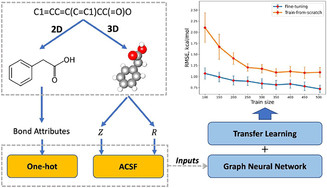
In this work, in order to address data scarcity of experimental aqueous solvation free energies, we first build a large and diverse calculated dataset Frag20-Aqsol-100K of aqueous solvation free energy with reasonable computational cost and accuracy via electronic structure calculations with continuum solvent models. Then we develop a novel DL model architecture based on graph neural network (GNN) and atomic 3D features (A3D). Based on molecular mechanics optimized geometries, A3D features were calculated by atom-centered symmetry functions (ACSF)³⁹ that are sets of many-body interaction functions encoding atomic environments in 3D structures. PNAConv as the GNN encoder combined with A3D features clearly demonstrate its superb learning power on the Frag20-Aqsol-100K. PNAConv is an advanced architecture combining multiple message aggregators with degree-scalers, which was originally proposed by Corso et al³⁶. Here we pre-trained the model on the Frag20-Aqsol-100K and employed the transfer learning strategy^40-42 on the experimental FreeSolv dataset. The fine-tuning performance by A3D-PNAConv-FT on FreeSolv achieved RMSE of 0.719 kcal/mol and a mean-absolute error (MAE) of 0.417 kcal/mol using multiple random data splits, which reaches the experimental uncertainty of 0.60 kcal/mol for MAE²¹. Moreover, our proposed model architecture with transfer learning strategy can make better predictions when given a training set with very small data size.

Datasets

For the experimental aqueous solvation free energy dataset, FreeSolv has been widely employed and benchmarked by various machine learning and deep learning models^1,14,21-34. FreeSolv consists of 642 neutral compounds, each of which is identified by the SMILES, IUPAC names along with the experimental values^1,14. The average and standard deviation of the experimental values are −3.82 kcal/mol and 4.84 kcal/mol, respectively.

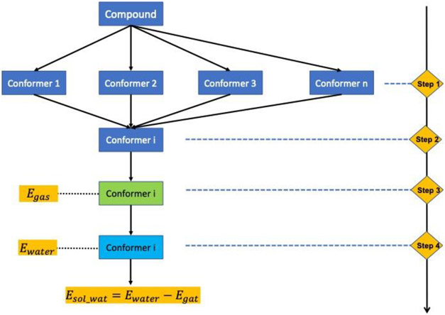
Since the data size of FreeSolv is very small, we build a large and diverse calculated dataset Frag20-Aqsol-100K for pre-training by employing a computation protocol as shown in Figure 1, which has achieved reasonable accuracy and computational cost. It should be noted that only a single conformer is used in this SMD-B3LYP computational protocol to calculate the solvation free energy, which can be further improved by considering an ensemble of conformation states. This SMD_B3LYP protocol yields an MAE of 1.28 kcal/mol in comparison with corresponding experimental aqueous solvation free energies for compounds in FreeSolv and this accuracy is comparable to other modeling studies^14,18. Frag20-Aqsol-100K contains 100K diverse compounds sampled from Frag20 and CSD20⁴², which consists of both molecular mechanics and B3LYP(6-31G*) optimized 3D geometries for molecules composed of H, B, C, O, N, F, P, S, Cl, and Br with no larger than 20 heavy atoms. The 3D geometry of each molecule in Frag20 was generated with RDKit⁴³(ETDKG⁴⁴) from Simplified Molecular-Input Line-Entry System (SMILES) representation and optimized by Merck Molecular Force Field⁴⁵ (MMFF) and then optimized and property-calculated using Density Functional Theory (DFT) method at B3LYP/6-31G* level. While for CSD20, the MMFF optimizations on the crystal structures were carried out, which was followed by DFT optimization, and molecular energy calculation.

Figure 1.

Computation protocol: SMD_B3LYP. Starting from the SMILE of a compound, a maximum of 300 conformers are generated by RDKit⁴³ using ETKDG⁴⁴ and optimized with MMFF94 force field⁴⁵(Step 1). The conformer i with the lowest MMFF energy is selected (Step 2). This conformer undergoes gas-phase optimization with B3LYP(6-31G*)⁴⁶ using Gaussian16⁴⁷ (Step 3). With the optimized geometry, the SMD¹⁵ calculation with B3LYP(6-31G*) in implicit water was carried out to calculate its aqueous solvation free energy (Step 4).

Methods

Model architecture

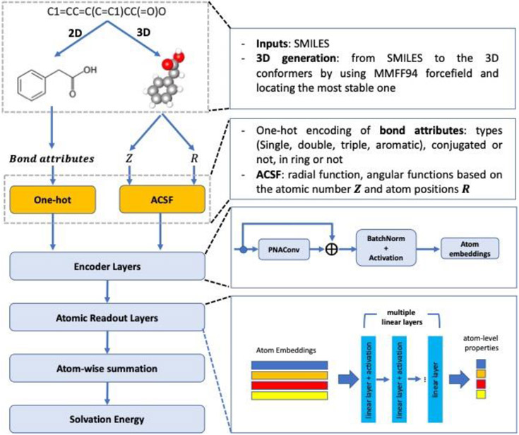
The general model architecture of A3D-PNAConv is shown in Figure 2. It basically has three principal components: molecule featurization, representation learning, and prediction blocks. The molecular featurization takes SMILES as inputs to generate both 3D structures and 2D graphs with explicit hydrogen atoms that are used to subsequently generate feature vectors for atoms and bonds. The encoder layers, which are used for atom embedding learning, mainly depend on the GNNs. Meanwhile, the skip-connection is applied on each GNN module and subsequently BatchNorm and activation function are applied on it as well. The atomic readout layers consist of multiple linear layers that supports the atom-level properties read-out from atom embeddings. Lastly, the atom-wise summation on the atom-level properties is used as the final predicted molecule-level properties such as solvation free energy in this work.

Figure 2.

A3D-PNAConv model architecture for predicting solvation free energy.

Initial featurization

In the A3D-PNAConv model, 3D atomic features (A3D) are calculated by atomic-centered symmetry functions (ACSFs) based on molecular mechanics optimized geometries. ACSFs are sets of many-body functions that encode atomic environments within a molecule³⁹ and have been used to predict molecular energy by Schutt et al⁴⁸. Liu et al. also used ACSF descriptors as the auxiliary prediction targets when predicting quantum properties in QM9 dataset⁴⁹. The three different two-body symmetry functions we used here are $G_i^{1,Z_1}$, $G_i^{2,Z_1}$, and $G_i^{4,Z_1,Z_2}$, as shown below. The radial functions $G_i^{2,Z_1}$ operate on the pairwise distances between atoms and can be formulated as sum of Gaussian functions multiplied by cutoff functions f_c, and the angular functions $G_i^{4,Z_1,Z_2}$ incorporate angles between combinations of three atoms and can be formulated as sum of cosine functions of the angle θ_ijk = (R_ij · R_ik/∣R_ij∣·∣R_ik∣) centered at atom i multiplied by Gaussian functions and cutoff functions f_c. All the summations on j for $G_i^{1,Z_1}$, $G_i^{2,Z_1}$ and on j, k for $G_i^{4,Z_1,Z_2}$ run over all atoms with specific atomic number.

$$\begin{gathered} G_i^{1,Z_1}={\sum }_j^{Z_1}{f}_c(R_{ij}) \\ {G}_i^{2,Z_1}={\sum }_j^{Z_1}{e}^{-\eta (R_{ij}-R_s{)}^2}\cdot f_c(R_{ij}) \\ {G}_i^{4,Z_1,Z_2}=2^{1-\zeta }{\sum }_{j\ne i}^{Z_1}{\sum }_{k\ne i}^{Z_2}(1+\lambda cos{\theta }_{ijk}{)}^{\zeta }\cdot e^{-\eta \left(R_{ij}^2+R_{ik}^2+R_{jk}^2\right)}\cdot f_c(R_{ij})\cdot f_c(R_{ik})\cdot f_c(R_{jk}) \\ {f}_c(R_{ij})=\{\begin{array}{c}0.5\cdot \left[cos\left(\frac{\pi R_{ij}}{R_c}\right)+1\right]\hfill \\ 0\hfill \end{array}\phantom{\}} \end{gathered}$$

For radial function, R_ij represents the distance between i and j, R_s is center of the Gaussian functions, η is the width of the Gaussian. For angular function, λ can have the values with +1 or −1, high values of ζ yield a narrower range, and η is used to control the radial distributions. The cutoff function ensures interactions decay to zero outside the cutoff R_c. Herein, the R_c value we adopted was always equal to 6.0. For 2D featurization on each bond, the bond attributes and the corresponding encoding methods are listed in Table S1.

Message Passing Neural Network (MPNN) and PNAConv

MPNN model works on undirected graphs G, which can be described by node attributes x_v and edge attributes e_vw. MPNN contains two phases: a message passing phase and a readout phase. The message passing phase incorporates information across the graphs to build a neural representation of the graphs, and the readout phase utilizes the final representation of the graphs to make predictions about the graph-level or node-level properties of interest⁵⁰.

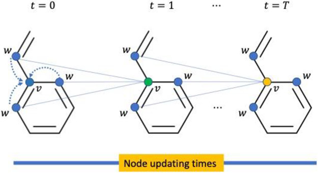
To be specific, the message passing phase runs for T steps. At each step t, the message function M_t generates messages $m_v^{t+1}$ for next iteration associated with each node, and the node update function U_t uses the messages to update the hidden state $h_v^t$ at each node in the graphs. The message function and node update function are shown below and in Figure 3:

$$\begin{gathered} m_v^{t+1}={\sum }_{w\in N(v)}{M}_t(h_v^t,h_w^t,e_{vw}) \\ {h}_v^{t+1}=U_t(h_v^t,m_v^{t+1}) \end{gathered}$$

where N(v) means the set of neighbors of v in graph G, and the initial hidden state $h_v^0$ is same with the initial node features x_v. The message function and updating functions for selected GNN modules that we applied are shown in Table S1. Typically, different GNN modules use slightly different MPNN mechanism to update node embeddings. Herein as for PNAConv³⁶, to construct the message function, it first applied node degree to construct a scaler that was multiplied by a combination of four aggregation methods (mean, max, min, standard deviation) to obtain the Principal Neighborhood Aggregation (PNA). The PNA works on the summation of the neighboring nodes’ embeddings, connected bonds’ embeddings and its own embeddings to generate the messages that are subsequently concatenated with the nodes themselves to update the node embedding. Specifically, the message function for PNAConv is:

$$m_v^{t+1}=M_t(h_v^t,h_w^t,e_{vw})=\oplus (h_v^t+h_w^t+e_{vw})$$

Figure 3.

Node updating in MPNN. At t = 0, all nodes are assigned with initial features. Then at t = 1, the node v’s feature gets updated by incorporating information from its neighboring nodes w. This updating is repeated several times.

⊕ represents PNA and is formulated as: $\oplus =\left[\begin{array}{c}\hfill I\hfill \\ \hfill S(d,\alpha =1)\hfill \\ \hfill S(d,\alpha =-1)\hfill \end{array}\right]\otimes \left[\begin{array}{c}\hfill \mu \hfill \\ \hfill \sigma \hfill \\ \hfill min\hfill \\ \hfill max\hfill \end{array}\right]$

where S(d, α) = ((log(d + 1)/δ)^α, d > 0, −1 ≤ α ≤ 1.δ is the normalization parameter and d is the node degree. The updating function for PNA is:

$$h_v^{t+1}=U_t(h_v^t,m_v^{t+1})=concat(h_v^t,m_v^{t+1})$$

where concat means the concatenation.

Implementation and Training Details

In this work, we compared 2D to 3D featurization on the atoms under six different GNN modules and showed their performance’s difference on the calculated data. For 2D featurization on atoms, the attributes and the corresponding encoding methods are listed Table S3. All 2D features for atoms and bonds are generated by RDKit⁴³, and 3D atomic features are generated from either MMFF-optimized or DFT-optimized 3D structures by Dscribe⁵¹ with the ACSF calculations, where g2_params were set to [[1,1], [1,2], [1,3]] for [η, R_s] in $G_i^{2,Z_1}$ function and g4_params were set to [[1, 1, 1], [1, 2, 1], [1, 1, −1], [1, 2, −1]] for [η, ζ, λ] in $G_i^{4,Z_1,Z_2}$ function. The initial feature sizes for 2D atoms, 2D bonds and 3D atoms are 50, 7, and 260, respectively.

We first pre-trained our models on the larger calculated dataset Frag20-Aqsol-100K such that we determined the best featurization method and GNN module. Then we fine-tuned the model on downstream experimental dataset FreeSolv. When fine-tuning the models, we initialized the models’ GNN parameters from the pre-trained models and retained the whole network. All trainings were implemented by Torch-Geometric framework⁵² and performed on RTX8000 GPU. All models were trained until it reaches 1000 epoch without early stopping, and were selected based on the smallest root-mean-squared error (RMSE) for the validation set. Hyper parameters for the model building and training are presented in Table S4. To be noted, except for the default internal hyper parameters of each GNN, we adopted same values for all other hyper parameters such as number of encoder layers, hidden size, loss function, etc.

Results and Discussion

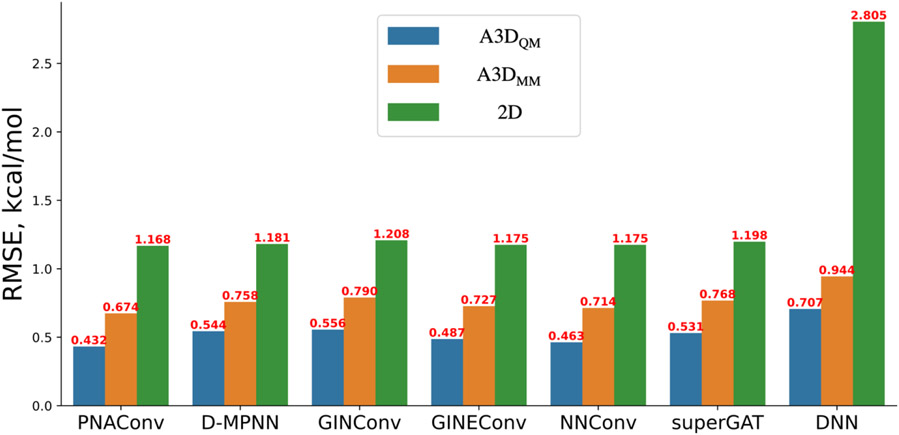
In order to compare different GNNs’ ability to learn molecular representation for solvation free energy prediction, we first built our models based on different GNN modules and trained them on Frag20-Aqsol-100K dataset, which was split into fixed train/validation/test sets with data size of 80K/10K/10K. The data distributions are shown in Figure S1 in the supporting information. The performances on the test set are shown below in Figure 4 and the statistical significance test is shown in Table S5.

Figure 4.

Performance on the test set of Frag20-Aqsol-100K by different GNN modules and DNN under A3D and 2D featurization methods. A3D_QM and A3D_MM are the A3D features that are calculated from DFT-optimized geometries and MMFF-optimized geometries, respectively. The value in red atop each bar are the mean RMSE on the test set by 5 runs with random weights initialization.

The results in Figure 4 and Table S5 clearly indicate that 3D atomic features obtained from molecular mechanics-optimized or DFT-optimized geometries can significantly improve the learning power of GNN based models in predicting calculated solvation free energies over 2D features. For all six GNN models that employ different message functions, including PNAConv³⁶, D-MPNN²⁶, GIN³⁵, GINE⁵³, NNConv⁵⁰, and superGAT⁵⁴ (see details in Table S2), they roughly showed a very similar performance of around 1.2 kcal/mol of RMSE using 2D atomic features as input, ranging from 1.168 kcal/mol for PNAConv to 1.208 kcal/mol for GINConv. As for DNN-based models, on the one hand, it is not surprising that using 2D atomic features with DNN alone would yield the worse result (RMSE = 2.805 kcal/mol) meaning that the 2D atomic feature itself encodes very little molecular information. On the other hand, using A3D features with DNN alone but without any message passing achieves a much better performance (0.944 kcal/mol for A3D_MM and 0.707 kcal/mol for A3D_QM), which clearly demonstrates that 3D atomic features encoded by atomic-centered symmetry functions (ACSFs) are excellent representations of atomic environments within a molecule. Our new finding here is that 3D atomic features obtained from molecular mechanics-optimized or DFT-optimized geometries can significantly improve the learning power of GNN models in predicting calculated solvation free energies, resulting in the performances of 0.674 kcal/mol for A3D_MM-PNAConv and 0.432 kcal/mol for A3D_QM-PNAConv. This is probably because energy related prediction tasks are highly dependent on the 3D structures of the molecules^48,55. The 2D features can only locally depicts the molecular topology rather than the complex inter-atomic relationship. Although A3D_QM-based models outperformed A3D_MM-based models because the calculated solvation free energies are based on the DFT-optimized geometries, the computational cost to obtaining DFT-optimized geometries is considerably expensive, which limits its applications in many scenarios. By comparing A3D and 2D features, it can be concluded that A3D can better help our model learn to predict aqueous solvation free energy by adequately describing the atomic environment in terms of many-body functions. Meanwhile, by using A3D features, all six GNN models achieve significant better results than A3D with DNN alone. These results indicates that message passing and edge information also play important roles in the atom embedding updating, which can further improve molecule representation learning for aqueous solvation free energy prediction. In the following parts, we use A3D for A3D_MM, unless indicated otherwise.

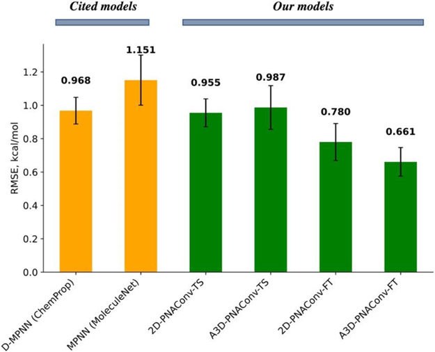
Considering that either using 2D features or A3D features, PNAConv has achieved slightly better performance than the other five GNN modules, we have used both 2D-PNAConv and A3D-PNAConv to test the transfer learning strategy for the experimental aqueous solvation free energy prediction. Here we first built our models based on PNAConv under 2D and A3D with the calculated dataset Frag20-Aqsol-100K and subsequently fine-tuned on the experimental dataset FreeSolv. We denoted the fine-tuned models 2D-PNAConv-FT and A3D-PNAConv-FT as the ones that were pre-trained on the calculated dataset Frag20-Aqsol-100K under 3D and 2D featurization, respectively. Based on the same data split (sizes for train/validation/test sets: 513/64/65) from the MoleculeNet²³, we removed 11 compounds in the training and 1 compound in the validation set that contain element iodine, and then used the rest 502/63/65 for our models’ training/validation/evaluation. We used the same data sets to train both 2D-PNAConv and A3D-PNAConv as well as two cited models D-MPNN (from ChemProp) and MPNN (from MoleculeNet), and the results are shown in Figure 5. The data distributions are available in Figure S2 in the supporting information.

Figure 5.

Performance on the fixed FreeSolv test set by different models. The values atop each bar are the mean RMSE on the test set by 5 runs with different initial weights. The error bars are the standard deviation of the mean across 5 runs. 2D-PNAConv-TS and A3D-PNAConv-TS means we trained PNAConv-based model from scratch using 2D and A3D features, respectively.

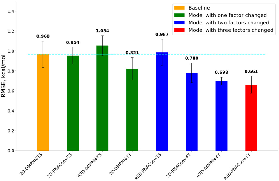
As we can see from Figure 5, the fine-tuned models 2D-PNAConv-FT and A3D-PNAConv-FT outperformed other train-from-scratch (TS) models, which indicates that the pre-training on a large, calculated data can improve the fine-tuning performance on the small, experimental data. Considering that A3D-PNAConv-FT achieved the best performance (Figure 5 & S3), we carried out the ablation studies on the selections of atomic featurization methods (2D vs A3D), GNN modules (PNAConv vs DMPNN) and training strategies (TS vs FT), as shown in Figure 6 and Table S6. We can see that the improvement of A3D-PNAConv-FT against the baseline model 2D-DMPNN-TS for FreeSolv is not due to one factor alone but is a combination of three factors. The transfer learning (fine tuning from the previously trained models on the calculate data set) looks to contribute more than the change of the other two factors.

Figure 6.

The ablation studies on the selections of atomic featurization methods (2D vs A3D), GNN modules (PNAConv vs DMPNN) and training strategies (TS vs FT). Starting from 2D-DMPNN-TS (baseline), we first changed one of the three factors (that said, atomic featurization methods, GNN modules and training strategies) and kept the other two factors constant. Then we changed two of the three factors and kept the left one constant. Lastly, we changed all the three factors. The dash cyan line shows the Baseline model’s RMSE.

Considering that FreeSolv is a very small dataset with experimental aqueous solvation free energy, we further tested A3D-PNAConv-FT using random data splits with ratio of 8/1/1 (data size: 504/63/63) and compared results with other reported models and frameworks in Table 1. We can see that A3D-PNAConv-FT achieved the state-of-the-art performance in terms of 10-fold cross-validation (CV) results on the test set of FreeSolv, with RMSE of 0.719 kcal/mol and MAE of 0.417 kcal/mol.

Table 1.

Performance of A3D-PNAConv-FT on the test set of FreeSolv with multiple random data splits in comparison with previously published models/frameworks.

Method/Framework	RMSE, kcal/mol	MAE, kcal/mol	References	Key notes
A3D-PNAConv-FT	0.719±0.168	0.417±0.066	This work
3DGCN	0.824±0.140	0.575±0.053	27	Feature matrix + inter-atomic position matrixa
AGBT	0.994±0.217	0.594±0.090	32	SMILES + structuresb
D-MPNN	1.075±0.054	-	26	2D features + molecular features, ChemProp
GraphConv	1.150±0.262	-	32, 56	Universal graph convolutional networks
AttentiveFP	1.091±0.191	-	25, 56	Graph attention + GRU
Weave	1.220±0.280	-	57, 23	GCN + Atom-pair features
FML	-	0.570	21	MD sampling + Kernel Ridge Regression

^aThe relative position matrix is designed to have the inter-atomic positions, rather than individual positions, that ensure translational invariance.

^bFor a given molecular structure and its SMILES strings, AG-FPs are generated from element-specific algebraic subgraphs module and BT-FPs are generated from a deep bidirectional transformer module, and then the random forest algorithm is used to fuse, rank, and select optimal fingerprints (AGBT-FPs) for machine learning.

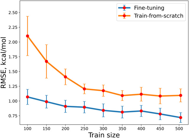
Lastly, to further examine the applicability of transfer learning strategy towards training data with even smaller size, we trained a series of fine-tuned models (A3D-PNAConv-FT) by changing the train size of FreeSolv and compared their 10-fold CV performance on the test set (63 samples) of FreeSolv using random data split of ratio 8/1/1 with corresponding training-from-scratch models (A3D-PNAConv-TS). As shown in Figure 7, when given a training set of very limited data size, A3D-PNAConv-FT can yield quite good performances. The results indicate that the fine-tuned models outperformed the train-from-scratch models on the experimental dataset with a very small data size, which points a promising direction for dealing with small experimental dataset in the future.

Figure 7.

Change of model performance on FreeSolv by A3D-PNAConv-TS and A3D-PNAConv-FT with different sizes of training set. The size of validation set was kept at 63. Each data point is the mean of 10-fold CV performance on the test set, and error bar represents its standard deviations.

Conclusion

At the early stages of drug discovery pipeline, data scarcity is the most common issue in the prediction of experimental physicochemical properties by deep learning models. As for experimental aqueous solvation free energy, very limited data could be used to train on to obtain a robust and reliable deep learning model. To tackle this problem, in this study we first built a calculated dataset of aqueous solvation free energy for 100K diverse compounds based on SMD calculations with reasonable accuracy and computation cost. Then we developed a novel deep learning model that was based on PNAConv and ACSF featurization of atoms to learn atom embeddings and generate powerful molecular representations for the solvation free energies. The developed A3D-PNAConv-FT model, which is pre-trained on the calculated dataset Frag20-Aqsol-100K achieving state-of-the-art performance on the FreeSolv (RMSE of 0.719 kcal/mol and MAE of 0.417 kcal/mol using random data splits with ratio of 8/1/1). In addition, with our developed model combined with the transfer learning strategy, it clearly demonstrated that the fine-tuned models outperformed the train-from-scratch models on the experimental dataset especially with very small data size, which points a promising direction for dealing with small experimental dataset in the future. However, it should be noted that the transfer learning approach applied here requires the development of a large, computed data set with reasonable accuracy, which is still an ongoing research topic and has not been achieved for many other molecular property prediction tasks.

Data and Software Availability

The calculated dataset Frag20-Aqsol-100K and the train/validation/test sets of FreeSolv are available in https://yzhang.hpc.nyu.edu/IMA. The data processing, model building and training have been implemented in a python package named EzChem, and are also accessible through: https://yzhang.hpc.nyu.edu/IMA. RDKit 2020.09 version, DScribe 1.2.0 version, PyTorch 1.7.1 version and PyTorch Geometrics are used to calculate initial 2D atom/bond features, 3D atom features and model building/training, respectively.

References

- 1.Matos GDR; Kyu DY; Loeffler HH; Chodera JD; Shirts MR; Mobley DL Approaches for Calculating Solvation Free Energies and Enthalpies Demonstrated with an Update of the FreeSolv Database. J. Chem. Eng. Data 2017, 62, 1559–1569. [DOI] [PMC free article] [PubMed] [Google Scholar]
- 2.Perlovich GL Thermodynamic Approaches to the Challenges of Solubility in Drug Discovery and Development. Mol. Pharmaceut 2014, 11, 1–11. [DOI] [PubMed] [Google Scholar]
- 3.Kim T; Park H Computational Prediction of Octanol–Water Partition Coefficient Based on the Extended Solvent-Contact Model. J. Mol. Graph. Model 2015, 60, 108–117. [DOI] [PubMed] [Google Scholar]
- 4.Skyner RE; McDonagh JL; Groom CR; van Mourik T; Mitchell JBO A Review of Methods for the Calculation of Solution Free Energies and the Modelling of Systems in Solution. Phys. Chem. Chem. Phys 2015, 17, 6174–6191. [DOI] [PubMed] [Google Scholar]
- 5.Chandrasekaran B; Abed SN; Al-Attraqchi O; Kuche K; Tekade RK Computer-aided prediction of pharmacokinetic (ADMET) properties. In: Dosage form design parameters, Academic Press, pp 731–755 [Google Scholar]
- 6.Daina A; Michielin O; Zoete V SwissADME: A Free Web Tool to Evaluate Pharmacokinetics, Drug-Likeness and Medicinal Chemistry Friendliness of Small Molecules. Sci Rep-uk. 2017, 7, 42717. [DOI] [PMC free article] [PubMed] [Google Scholar]
- 7.Yoshida N Role of Solvation in Drug Design as Revealed by the Statistical Mechanics Integral Equation Theory of Liquids. J. Chem. Inf. Model 2017, 57, 2646–2656. [DOI] [PubMed] [Google Scholar]
- 8.Liu J; Wang X; Zhang JZH; He X Calculation of Protein–Ligand Binding Affinities Based on a Fragment Quantum Mechanical Method. Rsc. Adv 2015, 5, 107020–107030. [Google Scholar]
- 9.Huang K; Luo S; Cong Y; Zhong S; Zhang JZH; Duan L An Accurate Free Energy Estimator: Based on MM/PBSA Combined with Interaction Entropy for Protein–Ligand Binding Affinity. Nanoscale. 2020, 12, 10737–10750. [DOI] [PubMed] [Google Scholar]
- 10.Han Y; Wang Z; Wei Z; Schapiro I; Li J Binding Affinity and Mechanisms of SARS-CoV-2 Variants. Comput. Struct. Biotechnology. J 2021, 19, 4184–4191. [DOI] [PMC free article] [PubMed] [Google Scholar]
- 11.Maggi N; Arrigo P; Ruggiero C Drug Design For Cardiovascular Disease: The Effect Of Solvation Energy On Rac1-Ligand Interactions. 2011 Annu Int Conf Ieee Eng Medicine Biology Soc 2011, 2011, 3237–3240. [DOI] [PubMed] [Google Scholar]
- 12.Nicholls A; Mobley DL; Guthrie JP; Chodera JD; Bayly CI; Cooper MD; Pande VS Predicting Small-Molecule Solvation Free Energies: An Informal Blind Test for Computational Chemistry. J. Med. Chem 2008, 51, 769–779. [DOI] [PubMed] [Google Scholar]
- 13.Zhang J; Zhang H; Wu T; Wang Q; van der Spoel D. Comparison of Implicit and Explicit Solvent Models for the Calculation of Solvation Free Energy in Organic Solvents. J. Chem. Theory Comput 2017, 13, 1034–1043. [DOI] [PubMed] [Google Scholar]
- 14.Mobley DL; Guthrie JP FreeSolv: A Database of Experimental and Calculated Hydration Free Energies, with Input Files. Journal of Computer-Aided Molecular Design 2014, 28, 711–720. [DOI] [PMC free article] [PubMed] [Google Scholar]
- 15.Marenich AV; Cramer CJ; Truhlar DG Universal Solvation Model Based on Solute Electron Density and on a Continuum Model of the Solvent Defined by the Bulk Dielectric Constant and Atomic Surface Tensions. J. Phys. Chem. B 2009, 13, 6378–6396. [DOI] [PubMed] [Google Scholar]
- 16.Voityuk AA; Vyboishchikov SF A Simple COSMO-Based Method for Calculation of Hydration Energies of Neutral Molecules. Physical Chemistry Chemical Physics 2019, 21, 18706–18713. [DOI] [PubMed] [Google Scholar]
- 17.Alibakhshi A; Hartke B Improved Prediction of Solvation Free Energies by Machine-Learning Polarizable Continuum Solvation Model. Nat. Commun 2021, 12, 3584. [DOI] [PMC free article] [PubMed] [Google Scholar]
- 18.Voityuk AA; Vyboishchikov SF Fast and Accurate Calculation of Hydration Energies of Molecules and Ions. Phys Chem Chem Phys. 2020, 22, 14591–14598. [DOI] [PubMed] [Google Scholar]
- 19.Klamt A; Eckert F; Arlt W COSMO-RS: An Alternative to Simulation for Calculating Thermodynamic Properties of Liquid Mixtures. Annu Rev Chem Biomol. 2010, 1, 101–122. [DOI] [PubMed] [Google Scholar]
- 20.Klamt A; Diedenhofen M Calculation of Solvation Free Energies with DCOSMO-RS. J Phys Chem. 2015, 119, 5439–5445. [DOI] [PubMed] [Google Scholar]
- 21.Weinreich J; Browning NJ; von Lilienfeld OA. Machine Learning of Free Energies in Chemical Compound Space Using Ensemble Representations: Reaching Experimental Uncertainty for Solvation. J Chem Phys. 2021, 154, 134113. [DOI] [PubMed] [Google Scholar]
- 22.Zang Q; Mansouri K; Williams AJ; Judson RS; Allen DG; Casey WM; Kleinstreuer NC In Silico Prediction of Physicochemical Properties of Environmental Chemicals Using Molecular Fingerprints and Machine Learning. J. Chem. Inf. Model 2017, 57, 36–49. [DOI] [PMC free article] [PubMed] [Google Scholar]
- 23.Wu Z; Ramsundar B; Feinberg EN; Gomes J; Geniesse C; Pappu AS; Leswing K; Pande V MoleculeNet: A Benchmark for Molecular Machine Learning. Chem. Sci 2017, 9, 513–530. [DOI] [PMC free article] [PubMed] [Google Scholar]
- 24.Coley CW; Barzilay R; Green WH; Jaakkola TS; Jensen KF Convolutional Embedding of Attributed Molecular Graphs for Physical Property Prediction. J. Chem. Inf. Model 2017, 57, 1757–1772. [DOI] [PubMed] [Google Scholar]
- 25.Xiong Z; Wang D; Liu X; Zhong F; Wan X; Li X; Li Z; Luo X; Chen K; Jiang H; Zheng M Pushing the Boundaries of Molecular Representation for Drug Discovery with the Graph Attention Mechanism. J. Med. Chem 2019, 63, 8749–8760. [DOI] [PubMed] [Google Scholar]
- 26.Yang K; Swanson K; Jin W; Coley C; Eiden P; Gao H; Guzman-Perez A; Hopper T; Kelley B; Mathea M; Palmer A; Settels V; Jaakkola T; Jensen K; Barzilay R Analyzing Learned Molecular Representations for Property Prediction. J. Chem. Inf. Model 2019, 59, 3370–3388. [DOI] [PMC free article] [PubMed] [Google Scholar]
- 27.Cho H; Choi IS Enhanced Deep-Learning Prediction of Molecular Properties via Augmentation of Bond Topology. Chemmedchem. 2019, 14, 1604–1609. [DOI] [PubMed] [Google Scholar]
- 28.Pathak Y; Laghuvarapu S; Mehta S; Priyakumar UD Chemically Interpretable Graph Interaction Network for Prediction of Pharmacokinetic Properties of Drug-Like Molecules. AAAI; 2020, 34, 873–880. [Google Scholar]
- 29.Vermeire FH; Green WH Transfer Learning for Solvation Free Energies: From Quantum Chemistry to Experiments. Chem. Eng. J 2021, 418, 129307. [Google Scholar]
- 30.Lim H; Jung Y Delfos: Deep Learning Model for Prediction of Solvation Free Energies in Generic Organic Solvents. Chem Sci. 2019, 10, 8306–8315. [DOI] [PMC free article] [PubMed] [Google Scholar]
- 31.Shen WX; Zeng X; Zhu F; li Wang Y; Qin C; Tan Y; Jiang YY; Chen YZ Out-of-the-Box Deep Learning Prediction of Pharmaceutical Properties by Broadly Learned Knowledge-Based Molecular Representations. Nat Mach Intell. 2021, 1–10. [Google Scholar]
- 32.Chen D; Gao K; Nguyen DD; Chen X; Jiang Y; Wei G-W; Pan F Algebraic Graph-Assisted Bidirectional Transformers for Molecular Property Prediction. Nat Commun. 2021, 12, 3521. [DOI] [PMC free article] [PubMed] [Google Scholar]
- 33.Li X; Fourches D Inductive Transfer Learning for Molecular Activity Prediction: Next-Gen QSAR Models with MolPMoFiT. J Cheminformatics. 2020, 1, 12–17. [DOI] [PMC free article] [PubMed] [Google Scholar]
- 34.Maziarka Ł; Danel T; Mucha S; Rataj K; Tabor J; Jastrzębski S Molecule Attention Transformer 2020. arXiv:2002.08264. arXiv.org e-Print archive. https://arxiv.org/abs/2002.08264 [Google Scholar]
- 35.Xu K; Hu W; Leskovec J; Jegelka S How Powerful Are Graph Neural Networks 2018? arXiv: 1810.00826. arXiv.org e-Print archive. https://arxiv.org/abs/1810.00826 [Google Scholar]
- 36.Corso G; Cavalleri L; Beaini D; Liò P; Veličković P Principal Neighbourhood Aggregation for Graph Nets 2020. arXiv:2004.05718. arXiv.org e-Print archive. https://arxiv.org/abs/2004.05718 [Google Scholar]
- 37.Dehmamy N; Barabási A-L; Yu R Understanding the Representation Power of Graph Neural Networks in Learning Graph Topology 2019. arXiv:1907.05008. arXiv.org e-Print archive. https://arxiv.org/abs/1907.05008 [Google Scholar]
- 38.Mater AC; Coote ML Deep Learning in Chemistry. J. Chem. Inf. Model 2019, 59, 2545–2559. [DOI] [PubMed] [Google Scholar]
- 39.Behler J Atom-centered symmetry functions for constructing high-dimensional neural network potentials. J. Chem. Phys 2011, 134, 074106. [DOI] [PubMed] [Google Scholar]
- 40.Cai C; Wang S; Xu Y; Zhang W; Tang K; Ouyang Q; Lai L; Pei J Transfer Learning for Drug Discovery. J. Med. Chem 2020, 63, 8683–8694. [DOI] [PubMed] [Google Scholar]
- 41.Wang Z; Liu M; Luo Y; Xu Z; Xie Y; Wang L; Cai L; Ji S MoleculeKit: Machine Learning Methods for Molecular Property Prediction and Drug Discovery 2020. arXiv:2012.01981. arXiv.org e-Print archive. https://arxiv.org/abs/2012.01981 [Google Scholar]
- 42.Lu J; Xia S; Lu J; Zhang Y Dataset Construction to Explore Chemical Space with 3D Geometry and Deep Learning. J. Chem. Inf. Model 2021, 61 (3), 1095–1104. [DOI] [PMC free article] [PubMed] [Google Scholar]
- 43.The RDKit: Open-Source Cheminformatics Software. http://www.rdkit.org (accessed Mar 2019).
- 44.Riniker S; Landrum GA Better Informed Distance Geometry: Using What We Know To Improve Conformation Generation. J. Chem. Inf. Model 2015, 55, 2562–2574. [DOI] [PubMed] [Google Scholar]
- 45.Halgren TA Merck Molecular Force Field. II. MMFF94 van Der Waals and Electrostatic Parameters for Intermolecular Interactions. J. Comput. Chem 1996, 17, 520–552. [Google Scholar]
- 46.Becke AD “Density-functional thermochemistry. III. The role of exact exchange,” J. Chem. Phys 1993, 98, 5648–5652. [Google Scholar]
- 47.Frisch MJTGW; Schlegel HB; Scuseria GE; Robb MA; Cheeseman JR; Scalmani G; Barone V; Mennucci B; Petersson GA; Nakatsuji H; Caricato M; Li X; Hratchian HP; Izmaylov AF; Bloino J; Zheng G; Sonnenberg JL; Hada M; Ehara M; Toyota K; Fukuda R; Hasegawa J; Ishida M; Nakajima T; Honda Y; Kitao O; Nakai H; Vreven T; Montgomery JA Jr.; Peralta JE; Ogliaro F; Bearpark M; Heyd JJ; Brothers E; Kudin KN; Staroverov VN; Kobayashi R; Normand J; Raghavachari K; Rendell A; Burant JC; Iyengar SS; Tomasi J; Cossi M; Rega N; Millam JM; Klene M; Knox JE; Cross JB; Bakken V; Adamo C; Jaramillo J; Gomperts R; Stratmann RE; Yazyev O; Austin AJ; Cammi R; Pomelli C; Ochterski JW; Martin RL; Morokuma K; Zakrzewski VG; Voth GA; Salvador P; Dannenberg JJ; Dapprich S; Daniels AD; Farkas O; Foresman JB; Ortiz JV; Cioslowski J; Fox DJ Gaussian 16, Gaussian Inc.: Wallingford, CT, 2016. [Google Scholar]
- 48.Schütt KT; Kessel P; Gastegger M; Nicoli KA; Tkatchenko A; Müller KR SchNetPack: A Deep Learning Toolbox For Atomistic Systems. J. Chem. Theory Comput 2018, 15, 448–455. [DOI] [PubMed] [Google Scholar]
- 49.Liu Z; Lin L; Jia Q; Cheng Z; Jiang Y; Guo Y; Ma J Transferable Multilevel Attention Neural Network for Accurate Prediction of Quantum Chemistry Properties via Multitask Learning. J. Chem. Inf. Model 2021, 61 (3), 1066–1082. [DOI] [PubMed] [Google Scholar]
- 50.Gilmer J; Schoenholz SS; Riley PF; Vinyals O; Dahl GE Neural Message Passing for Quantum Chemistry 2017. arXiv: 1704.01212. arXiv.org e-Print archive. https://arxiv.org/abs/1704.01212 [Google Scholar]
- 51.Himanen L; Jäger MOJ; Morooka EV; Canova FF; Ranawat YS; Gao DZ; Rinke P; Foster AS DScribe: Library of Descriptors for Machine Learning in Materials Science. Comput. Phys. Commun 2020, 247, 106949. [Google Scholar]
- 52.Fey M; Lenssen JE Fast Graph Representation Learning with PyTorch Geometric 2019. arXiv: 1903.02428. arXiv.org e-Print archive. https://arxiv.org/abs/1903.02428 [Google Scholar]
- 53.Hu W; Liu B; Gomes J; Zitnik M; Liang P; Pande V; Leskovec J Strategies for Pre-Training Graph Neural Networks 2019. arXiv: 1905.12265. arXiv.org e-Print archive. https://arxiv.org/abs/1905.12265 [Google Scholar]
- 54.Schütt KT; Arbabzadah F; Chmiela S; Müller KR; Tkatchenko A Quantum-Chemical Insights from Deep Tensor Neural Networks. Nat. Commun 2017, 8, 13890. [DOI] [PMC free article] [PubMed] [Google Scholar]
- 55.Kim D; Oh A How to find your friendly neighborhood: graph attention design with self-supervision. ICLR 2021. [Google Scholar]
- 56.Jiang D; Wu Z; Hsieh C-Y; Chen G; Liao B; Wang Z; Shen C; Cao D; Wu J; Hou T Could Graph Neural Networks Learn Better Molecular Representation for Drug Discovery? A Comparison Study of Descriptor-Based and Graph-Based Models. J Cheminformatics. 2021, 13, 12. [DOI] [PMC free article] [PubMed] [Google Scholar]
- 57.Kearnes S; McCloskey K; Berndl M; Pande V; Riley P Molecular Graph Convolutions: Moving beyond Fingerprints. J Comput Aid Mol Des. 2016, 30, 595–608. [DOI] [PMC free article] [PubMed] [Google Scholar]
Associated Data
This section collects any data citations, data availability statements, or supplementary materials included in this article.
Supplementary Materials
Data Availability Statement