Abstract
Computer-aided drug design uses high-performance computers to simulate the tasks in drug design, which is a promising research area. Drug–target affinity (DTA) prediction is the most important step of computer-aided drug design, which could speed up drug development and reduce resource consumption. With the development of deep learning, the introduction of deep learning to DTA prediction and improving the accuracy have become a focus of research. In this paper, utilizing the structural information of molecules and proteins, two graphs of drug molecules and proteins are built up respectively. Graph neural networks are introduced to obtain their representations, and a method called DGraphDTA is proposed for DTA prediction. Specifically, the protein graph is constructed based on the contact map output from the prediction method, which could predict the structural characteristics of the protein according to its sequence. It can be seen from the test of various metrics on benchmark datasets that the method proposed in this paper has strong robustness and generalizability.
Prediction of drug–target affinity by constructing both molecule and protein graphs.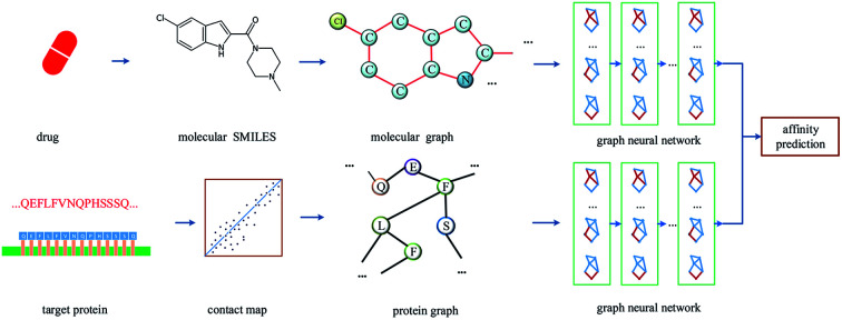
1. Introduction
The high performance of computers allows them to provide assistance for laboratory experiments in drug design.1 So computer-aided drug design has been developed in the past few decades. This makes full use of high-performance computers, which can quickly simulate the many steps in drug design, and various applications have been gradually developed. For instance, NAMD (NAnoscale Molecular Dynamics),2 GROMACS3 and Amber4 provide relatively accurate molecular dynamics simulation means, which can simulate the natural motion of a molecular system under defined conditions. Molecular docking can explore the binding conformational space between different molecules, and help researchers to find the optimal docking conformation. There are many methods that focus on molecular docking including DOCK,5 AutoDock,6 GOLD7 and so on. With the excellent achievements of deep learning in various fields, there are a variety of drug design applications and models emerging based on it. Preuer et al. constructed a feed forward neural network and proposed a model called DeepSynergy8 to predict anti-cancer drug synergy. DeepTox,9 composed of a deep neural network, was proposed for toxicity prediction and performed well in Tox21 challenge dataset.10 BSite-pro11 used a random forest classifier to predict the protein binding site based on the sequence alone. Lenselink et al. proved that deep neural networks outperformed a bioactivity benchmark set.12 Ciriano et al. summarized the recent proteochemometric modelling based on machine learning.13 DEEPScreen used deep convolutional neural networks to find a new target of the well-known drug cladribine.14 DeepDTIs used unsupervised pretraining to build a classification model to predict whether a drug can interact with an exiting target or a drug.15 Using deep learning for molecular modelling functions has gradually become a trend, because it can capture hidden information that is difficult to simulate according to human experience.
Virtual screening is a very common strategy in computer-aided drug design, which has been widely used. Drug–target affinity (DTA) prediction is an important step in virtual screening, which can quickly match target and drug and speed up the process of drug development. DTA prediction provides information about the binding strength of drugs to target proteins, which can be used to show whether small molecules can bind to proteins. For proteins with known structure and site information, we can use molecular simulation and molecular docking to carry out detailed simulations, thus get more accurate results, which is called structure-based virtual screening.16–18 Nevertheless, there are still many proteins for which there is no structural information. Even using homology modelling, it is still difficult to acquire structural information of many proteins. So it is an urgent problem to predict protein binding affinity with drug molecules using sequences (sequence-based virtual screening), which is also the focus of this paper. Due to the complicated structure of proteins and small molecules, accurate description and feature of target and drug is the most difficult part of affinity prediction, which is also a research hotspot in computer-aided medicine, especially with the rise of deep learning in the past decade.
At present, most of the latest sequence-based virtual screening prediction algorithms are based on deep learning. More specifically, for any pair of drug–target entries, the deep learning method is utilized to extract the representations of drug and target respectively, which will be concatenated into one vector for final prediction. In some cases, DTA prediction is treated as a binary problem. The model is a binary classifier used for determining whether the drug can bind to the target or not, such as NRLMF,19 KronRLS-MKL,20 and SELF-BLM.21
With the improvement of the accuracy of neural network and the increasing demands of high-precision drug design, accurate DTA prediction has received more and more attention, in which DTA is regarded as a regression problem. The output is the binding affinity between drug and target, and dissociation constants (Kd),22 inhibition constants (Ki)23 or the 50% inhibitory concentrations (IC50)22 are commonly used to measure the strength. Currently, there are some methods that have achieved good performance in affinity prediction. For example, DeepDTA24 constructed two convolutional neural networks (CNN) to extract the representations of the drug and the protein respectively, finally the two representations being concatenated to predict the affinity. In addition, DeepDTA collected previous data and built two benchmark datasets, where the drug is expressed as SMILES and protein is described through sequence. Two convolution networks were designed to obtain the representations of molecule and protein respectively, which achieved good results in the benchmark. WideDTA25 was further improved on the basis of DeepDTA, in which Live Max Common Substructure (LMCS) and Protein Motifs and Domains (PDM) were introduced and four CNNs were used to encode them into four representations. Huang et al. proposed a novel fingerprint feature vector for the molecule and the protein sequence was represented as a Pseudo Substitution Matrix Representation (Pseudo-SMR) descriptor for drug–target interaction prediction.26 In addition, Lee et al. compared different target features for predicting drug–target interactions.27 For molecule representation, molecular fingerprint is a common way, which can encode the structure of a molecule into a string or binary digits, such as extended connectivity fingerprints,28 atom environment descriptors (MOLPRINT2D)29 and molecular access system keys (MACCS).30 MoleculeNet provided lots of open-source tools of molecular featuring and learning algorithms, which also can be used for molecule representation.31 Altae-Tran et al. reported how to learn meaningful small-molecule representations when there are lower amounts of data.32 There are also many works attempting to characterize proteins. Westen et al. summarized a total of 13 different protein descriptor sets.33 DeepLSTM represented proteins using position-specific scoring matrix (PSSM) and Legendre moment.34
Moreover, the graph neural network (GNN) has been widely used in various fields. A graph composed of nodes and edges is used as the input of GNN and there is no limit to the size of the input graph, which provides a flexible format to extract in-depth information of molecules. Graph convolutional network (GCN)35 and graph attention network (GAT)36 are widely used GNN models, and they have been gradually applied in computer-aided drug design, such as drug property prediction37 and molecular fingerprint generation.38 In addition, PADME utilized molecular graph convolution in drug–target interaction prediction, which suggests the potential of GNN in drug development.39 Similarly, GraphDTA40 introduced GNN into DTA prediction, which constructed a graph with atoms as nodes and bonds as edges to describe drug molecules. CNN was used to extract protein sequence representation, and GNN models were implemented on the molecular graph, which improved the DTA prediction performance.
But in GraphDTA, CNN was used to obtain protein features through the sequence, which did not construct a graph for each protein. Proteins contain a large number of atoms, and if the graph of a protein is constructed with atoms as nodes, its structure will be very large and the cost of training very high. If the graph of a protein is constructed with residues as nodes, the constructed graph is only a long chain linked by peptide bonds, which cannot be regarded as a graph for calculation. Therefore, building a protein graph through a protein sequence is an ongoing problem to be solved.
Actually, a protein is not only a chain, but also a folded and complex structure formed by non-bonded interactions such as hydrogen bonds and van der Waals forces. If the spatial structure of a protein can be predicted and described through its sequence, it will be helpful for DTA prediction. Inspired by GraphDTA, GNN is also introduced in this work for DTA prediction. But unlike GraphDTA, we have not only constructed the graph of the drug molecule, but also constructed the protein graph. The number of residues of a protein is about several hundred, so it is suitable to construct graph with residues as nodes. However, the connection of residues is only a long chain without any spatial information. So the contact map is introduced in this paper. The contact map is a kind of representation of a protein structure, which is a 2D (two-dimensional) representation of the 3D (three-dimensional) protein structure,41 and it is often used as the output of protein structure prediction. More importantly, the output contact map, usually a matrix, is exactly consistent with the adjacency matrix in GNNs, which provides an efficient way to combine both data sources together. Therefore, how to introduce the contact map into the protein graph construction to improve the performance of affinity prediction is the focus of this work.
In order to bridge the huge gap between the speed of structure analysis and the speed of sequencing, protein structure prediction methods have emerged. These methods predict the 3D structure of proteins by mining the hidden information in the protein sequences. Contact maps (or distance maps) are the prediction results of many protein structure prediction methods, which show the interaction of residue pairs in the form of a matrix. Raptor-X-Contact42 integrated both evolutionary coupling and sequence conservation information and used residual neural networks to predict protein contact maps. DNCON2,43 which consists of six CNNs, used various distance thresholds as features to improve precision and achieved a great performance in contact map prediction. SPOT-contact44 utilized residual networks to congregate the short-range relations and 2D Bidirectional-ResLSTMs and proved its usefulness in contact prediction. Currently, there are other protein structure prediction methods, such as DeepContact,45 DeepConPred,46 MetaPSICOV,47 CCMpred,48etc., which also have good performance. Nevertheless, these methods need to install a large number of dependencies, which could slow down the process of contact map prediction for large-scale proteins, and thus they are not suitable for contact map prediction for DTA prediction. Pconsc4 (ref. 49) is a fast, simple and efficient contact map prediction method, and its performance is consistent with that of the current state of the art methods. Therefore, Pconsc4 is introduced in this paper to construct protein contact map and protein graph.
In the interaction between protein and drug molecule, the structural information will directly affect their binding strength. The protein structure can be obtained by crystallization in the laboratory, and the process takes a lot of time and labor costs. In drug design, especially in DTA prediction, a large number of protein structures are unknown, and only the protein sequence is used as the input for the prediction method. So protein structure prediction, the output of which is the contact map, is utilized in this paper which provides more structural information for DTA. The protein graph based on the contact map of the protein is constructed firstly, and a new method called DGraphDTA (double graph DTA predictor) is proposed for DTA prediction, which encodes both small drug molecule and protein using GNN. As far as we know, the proposed method is the first attempt to construct a protein graph based on the contact map of the protein. We apply GNNs on both protein and molecular graphs to improve performance, and obtain good prediction results in the benchmark datasets.
2. Materials and methods
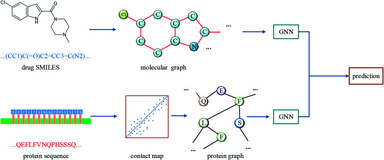
The overall architecture of DGraphDTA is inspired by the previous DTA prediction method24,25,40 based on deep learning, which extracts the representations of drug molecule and protein, then concatenates them for prediction. The innovation of the proposed method is the introduction of a novel graph to represent the protein, which could better describe its structure and features. The architecture is shown in Fig. 1. It can be seen from the figure that the graph constructed for extracting the small-molecule representation is basically same as that of GraphDTA. But for the process of the protein, the contact map is first predicted from the protein sequence, and a protein graph is then constructed based on it. After that, two GNNs are used to obtain the representations of the two graphs. In addition, unlike GraphDTA, we proposed a unified model architecture for all datasets, so that the model can be implemented conveniently.
Fig. 1. The architecture of DGraphDTA. Drug molecule SMILES is used for molecule construction and the graph is built up based on it. For the protein, the contact map is constructed based on the protein sequence, and then the graph is built up. After getting two graphs, they enter two GNNs to extract the representations. Finally the representations are concatenated for affinity prediction.
2.1. Datasets
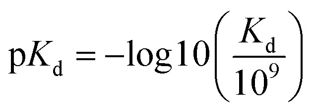
The benchmark datasets proposed by DeepDTA are used for performance evaluation. The benchmark includes Davis50 and KIBA51 datasets. The Davis dataset contains selected entries from the kinase protein family and the relevant inhibitors with their respective dissociation constant Kd values. The KIBA dataset contains combined kinase inhibitor bioactivities from different sources such as Ki, Kd and IC50 and the bioactivities are processed using KIBA score which is used for training and prediction. The protein and drug molecule entries in the two datasets are shown in Table 1. In the benchmark, each dataset is divided to six parts, one for testing and the other five for cross training and validation. Similar to DeepDTA, the pKd calculated through eqn (1) is used for Davis dataset affinity prediction:
 |
1 |
Datasets.
| Number | Dataset | Proteins | Compounds | Binding entities |
|---|---|---|---|---|
| 1 | Davis | 442 | 68 | 30 056 |
| 2 | KIBA | 229 | 2111 | 118 254 |
Because of the limitation of memory, only one large protein and its related entries were removed from the KIBA dataset. Through testing on the two datasets, the prediction performance of the method can be measured comprehensively.
2.2. Molecule representation
In the datasets, an affinity entry contains a molecule–protein pair. The drug molecule is described using SMILES. In the proposed method, the molecular graph is constructed according to the drug SMILES string, which takes atoms as nodes and bonds as edges. In order to ensure that the features of nodes can be fully considered in the process of graph convolution, the self-loops are also added into graph construction to improve the feature performance of the drug molecule. The graph construction for the molecule is shown in Fig. 2. The selected molecular features are the same as those in GraphDTA, which is illustrated in Table 2.
Fig. 2. Construction of molecular graph. The SMILES of the drug molecule is inputted and the molecular graph is constructed with atoms as nodes and bonds as edges, and then the related adjacency matrix is generated. In order to involve the convolution of the atom itself, the self-loop is added, that is, the diagonal of the adjacency matrix is set to 1.
Node features (atom).
| Number | Feature | Dimension |
|---|---|---|
| 1 | One-hot encoding of the atom element | 44 |
| 2 | One-hot encoding of the degree of the atom in the molecule, which is the number of directly-bonded neighbors (atoms) | 11 |
| 3 | One-hot encoding of the total number of H bound to the atom | 11 |
| 4 | One-hot encoding of the number of implicit H bound to the atom | 11 |
| 5 | Whether the atom is aromatic | 1 |
| All | 78 |
2.3. Protein representation
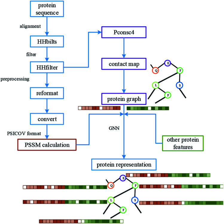
For protein representation, we use GNN to extract its latent vector, which requires the construction of the graph of the protein and the selection of node features. So, similar to the processing of the drug molecule, the first step of the protein representation extraction is to obtain the protein graph, then the representation can be extracted after the GNN on the protein graph. Fig. 3 illustrates the process of graph generation. Because the generation of protein graph and features depends on the sequence alignment result, a pre-processing has been introduced, including sequence alignment, sequence screening and other steps, which is illustrated in Fig. 4.
Fig. 3. Construction of protein graph. The protein sequence was preprocessed first, then the contact map was predicted by Pconsc4, then the adjacency matrix of the protein graph was obtained after threshold (0.5) filter.
Fig. 4. The processing of protein, including the pre-processing of the sequence, graph construction and feature generation. The results of protein sequence alignment and filter were fed into Pconsc4 for contact map prediction. After further format conversion, the filtered results are used for PSSM calculation.
The purpose of protein structure prediction is to analyse and construct the 3D structure of the protein according to the protein sequence. The structural information of a protein contains the connection angle and distance of different residue pairs. The contact map is a kind of output of structure prediction methods, which is usually a matrix. Assuming that the length of the protein sequence is L, then the predicted contact map M is a matrix with L rows and L columns, where each element mij of M indicates whether the corresponding residue pair (residue i and residue j) is contacted or not. Generally speaking, two residues are considered to be in contact if the Euclidean distance between their Cβ atoms (Cα atoms for glycine) is less than a specified threshold.41 In this paper, Pconsc4 is used to predict the contact map, which is a fast, simple, open-source and efficient method.
The model of Pconsc4 is implemented using U-net architecture,52 which operates on the 72 features calculated from each position in the multiple sequence alignment. The output of Pconsc4 is the probability of whether the residue pair contacts, then a threshold of 0.5 is set to get the contact map with a shape of (L, L), where L is the number of nodes (residues). The result just corresponds to the adjacency matrix of the protein. In the obtained adjacency matrix, the spatial information of protein is well preserved which can be extracted effectively through GNN.
After getting the adjacency matrix of the protein, the node features need to be extracted for further processing. Because the graph is constructed with the residue as the node, the feature should be selected around the residue, which shows different properties due to the different R groups. These properties include polarity, electrification, aromaticity and so on. In addition, PSSM53 is a common representation of proteins in proteomics. In PSSM, each residue position can be scored based on sequence alignment result, which is used to represent the feature of residue node. To sum up, 54 bit features are used in this paper to describe the residue node. Details of these features are shown in Table 3. Then the shape of node features is (L, 54). And the adjacency matrix and node features are processed through GNN to obtain the vector representation of the corresponding protein.
Node features (residue).
| Number | Feature | Dimension |
|---|---|---|
| 1 | One-hot encoding of the residue symbol | 21 |
| 2 | Position-specific scoring matrix (PSSM) | 21 |
| 3 | Whether the residue is aliphatic | 1 |
| 4 | Whether the residue is aromatic | 1 |
| 5 | Whether the residue is polar neutral | 1 |
| 6 | Whether the residue is acidic charged | 1 |
| 7 | Whether the residue is basic charged | 1 |
| 8 | Residue weight | 1 |
| 9 | The negative of the logarithm of the dissociation constant for the –COOH group64 | 1 |
| 10 | The negative of the logarithm of the dissociation constant for the –NH3 group64 | 1 |
| 11 | The negative of the logarithm of the dissociation constant for any other group in the molecule64 | 1 |
| 12 | The pH at the isoelectric point64 | 1 |
| 13 | Hydrophobicity of residue (pH = 2)65 | 1 |
| 14 | Hydrophobicity of residue (pH = 7)66 | 1 |
| All | 54 |
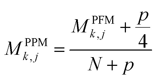
For PSSM calculation, in order to decrease computation time, its simplified calculation has been implemented. At first, a basic position frequency matrix (PFM)53 is created by counting the occurrences of each residue at each position, which is illustrated in eqn (2):
 |
2 |
where A is a set of N aligned sequences for a protein sequence with length of L, k belongs to residue symbols set, i = (1, 2, …, N), j = (1,…, L) and I(x) is an indicator function when the condition x is satisfied and 0 otherwise. Then a position probability matrix (PPM)54 can be obtained using eqn (3):
 |
3 |
where p is the added pseudocount54 to avoid matrix entries with value of 0, which is set to 0.8. Then, the PPM is used as PSSM to represent a part of the features of residue node.
When running the program of Pconsc4 and calculating PSSM, the input is the result of protein sequence alignment. So in the pre-processing stage, the alignments of all proteins in the benchmark datasets need to be done at first. In order to increase the computation speed, HHblits55 is used to carry out the protein sequence alignment. After alignment, the HHfilter55 and the CCMPred48 scripts are implemented on the results to get alignments in the PSICOV56 format.
2.4. Model architecture
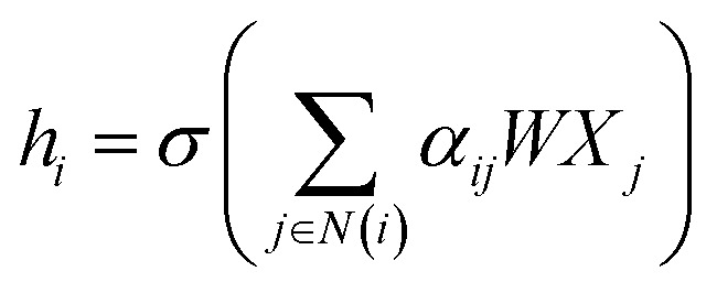
CNNs can only operate on regular Euclidean data like images (2D grid) and text (1D sequence), and the restrictions on the use of CNNs limit their application in some non-Euclidean fields. GNNs are powerful neural networks, which aim to directly process graphs and make use of their structural information. After several years of rapid development, GNN has derived many powerful variants, such as GCN and GAT. These models are very effective for the feature extraction of graphs. For GCN, each layer will carry out a convolution operation through eqn (4):
 |
4 |
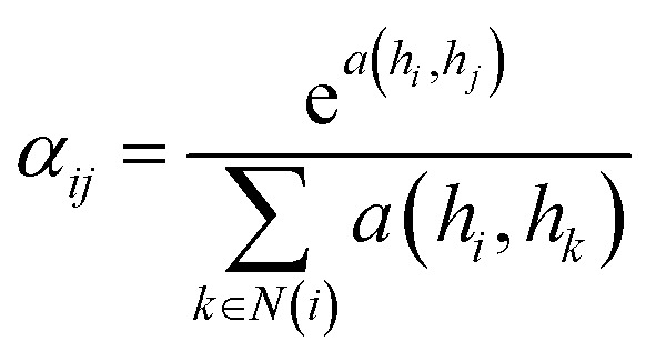
where A is the adjacency matrix of the protein graph with the shape (n, n), n is the number of the nodes in the graph, Â = A + I, I is the identity matrix, D̂ is the diagonal node degree matrix calculated from A, and with the same shape as A, Wl+1 is the weight matrix of the layer l + 1, Hl is the last layer output with a shape (n, Fl), Fl is the number of the output channels in layer l and H0 = X. X is the input the feature vector of the nodes. For GAT, in each layer, the node feature can be calculated as:
 |
5 |
 |
6 |
where N(i) is the set of neighbors of node i, W is the weight matrix, Xj the feature vector of node j and αij is the normalized attention coefficients calculated as eqn (6). a(·) is a map of RFl × RFl → R, which computes non-normalized coefficients across pairs of nodes i, j.
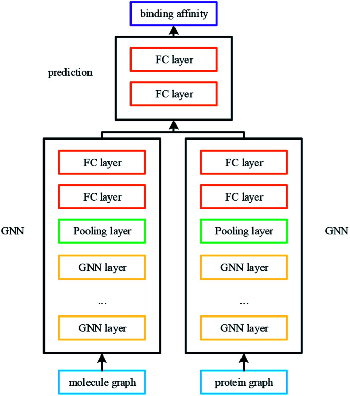
In DGraphDTA, GNNs are introduced to obtain the representations of molecule and protein. Fig. 5 shows the model architecture. In our experiment, we found that it is most effective to extract the features of small molecules and proteins by using three-layer convolution network. Implementation details can be found in the experiment part.
Fig. 5. The network of DGraphDTA. The graphs of molecule and protein pass through two GNNs to get their representations. Then the affinity can be predicted after multiple fully connected layers.
Unified GNN model is constructed for different datasets, so the proposed method is simple and easy to implement. After the graphs of drug molecule and protein are constructed, they are fed into two GNNs for training. After convolution of multiple GNN layers, the representations of both molecule and protein are effectively extracted. Then the overall features of the corresponding small molecule–protein pair for DTA prediction are obtained. Finally, the prediction is carried out through two full connection layers.
For small drug molecules, the atoms that compose a molecule are connected by covalent bonds, and different atoms and structures will eventually behave as different molecular properties and interact with the outside world through the connections. Therefore, using graph convolution, the relations between these different atoms are fully considered, so the representation of the molecule will be effectively extracted.
For protein graph, another GNN is used to extract the representation. There is much spatial information in the protein structure, which is important for the binding affinity of protein and molecule. The protein contact map obtained by the structure prediction method can extract the information of each residue, which is mainly reflected in the relative position and interaction of residue pairs. The interaction of these residue pairs can fully describe the spatial structure of proteins through the vectors obtained by GNN. In computer-aided drug design, it is a difficult task to obtain the representation of a protein only by sequence. By using GNN, DGraphDTA can map the protein sequence to the representation with rich features, which provides an effective method for feature extraction of proteins. The proposed method utilized Pconsc4 to construct the topological structure of the protein on the premise of only knowing the sequence, and discovering the hidden information of the whole structure of the protein which is useful for affinity prediction. In addition, there are many factors that affect the performance of network structure, such as the number of network layers, the choice of GNN model and the probability of dropout. Because the training process needs a lot of time, some hyperparameters are selected by human experience. For other important hyperparameters, comparison and determination were implemented in the experimental part.
For each graph of molecule and protein, the dimension of the feature of each node is fixed, but the number of nodes of each graph is not fixed which depends on the number of atoms or residues. So the size of the GNN output matrix varies with the number of nodes and global pooling is added after the two GNNs to ensure that the same size of representation can be output for proteins and molecules with different node numbers. Supposing the last GNN layer outputs the protein representation with shape (L, Fl), then the global pooling can be calculated as:
| Hpi = pool (Hl(i)) | 7 |
where Hl(i) is the ith column of Hl, i = 1, 2, …, Fl and pool is the pooling operation, which can be calculated as sum, mean or max. Then the latent representation of the protein can be obtained with shape (1, Fl), which is independent of protein size. Different types of global pooling are compared as hyperparameters to verify the impact of prediction performance in our experiment.
3. Results and discussion
DGraphDTA is built with PyTorch,40 which is an open source machine learning framework. The GNN models are implemented using PyTorch geometric (PyG).41 For drug molecules, due to their small structure, the performances of different models are similar. For the protein, there are lots of residue nodes, so the choice of model is very important. Therefore, multiple experiments are used to select the hyperparameters with a 5-fold cross validation. When the hyperparameters are determined by the cross validation, we used all 5 folds training sets and test set in benchmark to train and test DGraphDTA for performance evaluation. At the same time, various methods and metrics are introduced for comparison.
3.1. Metrics
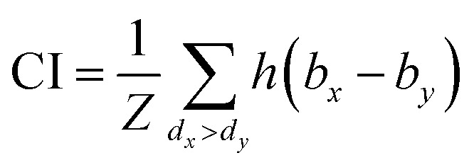
The same metrics in the benchmark were implemented, which calculates the concordance index (CI)57 and mean squared error (MSE).58 CI is mainly used to calculate the distinction between the predicted value and the real value in the analysis, which is calculated through eqn (8):
 |
8 |
 |
9 |
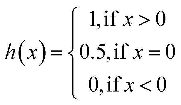
where bx is the prediction value for the larger affinity dx, by is the prediction value for the smaller affinity dy, and Z is a normalization constant; h(x) is the step function, which is illustrated in eqn (9).
MSE is also a common metric to measure the difference between the predicted value and the real value. For n samples, the MSE is calculated as the average of the sum of the square of the difference between the predicted value pi (i = 1, 2,…,n) and the real value yi. A smaller MSE means that the predicted values of the sample are closer to the real values:
 |
10 |
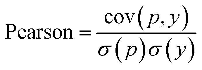
In WidedDTA, another metric, the Pearson correlation coefficient,59 is used for performance comparison, which is calculated through eqn (11). In the equation, cov is the covariance between the predicted value p and the real value y, and σ indicates the standard deviation. In our experiment, the metric is also introduced to evaluate the prediction performance of the proposed method.
 |
11 |
In addition, the metric rm2 index60 is involved in DeepDTA, which is also introduced as a measure in the proposed method. The calculation of rm2 is described in eqn (12):
 |
12 |
where r2 and r02 are the squared correlation coefficients with and without intercept respectively.
3.2. Setting of the hyperparameters
Training a model requires hyperparameter settings, and there are also many hyperparameters in DGraphDTA. Because it takes several hours to train a model, some of the parameters are set by human experience, while other important parameters are compared in the following experiments. The human experience hyperparameter settings are shown in Table 4.
The hyperparameter settings using human experience.
| Hyperparameter | Setting |
|---|---|
| Epoch | 2000 |
| Batch size | 512 |
| Learning rate | 0.001 |
| Optimizer | Adam |
| Fully connected layers after GNN | 2 |
| Fully connected layers after concatenation | 2 |
3.3. Performances of various GNN models
In order to improve the precision of the DTA prediction, it is very important to choose an effective GNN model to describe the protein at the first step. The most important factors that affect the performance of model include the architecture of GNN and the number of layers. Therefore, two architectures (GCN and GAT) and different numbers of layers are implemented for performance comparison. The detailed implementation is shown in Table 5, including 8 combinations. The Davis database is used for the experiment. Because there are hundreds or even thousands of nodes in the protein graph, too many layers will lead to using up of memory for the graphic card. So only up to three layers are tested. Different GNN model performances are shown in Table 6.
Combinations of various GNN models on Davis dataset.
| Model | Number of layers | Layer1(in, out, head) | Layer2(in, out, head) | Layer3(in, out, head) |
|---|---|---|---|---|
| GCN | 1 | GCN(54, 54) | — | — |
| GCN | 2 | GCN(54, 54) | GCN(54, 108) | — |
| GCN | 3 | GCN(54, 54) | GCN(54, 108) | GCN(108, 216) |
| GAT | 1 | GAT(54, 54, h = 2) | — | — |
| GAT | 2 | GAT(54, 54, h = 2) | GAT(54, 108, h = 2) | — |
| GAT | 3 | GAT(54, 54, h = 2) | GAT(54, 108, h = 2) | GAT(108, 216, h = 2) |
| GAT&GCN | 1&1 | GAT(54, 54, h = 2) | GCN(54, 108) | — |
| GCN&GAT | 1&1 | GCN(54, 54) | GAT(54, 108, h = 2) | — |
Performances of various GNN models on Davis dataset.
| Model | Number of layers | CI (std) | MSE (std) | Pearson (std) |
|---|---|---|---|---|
| GCN | 1 | 0.891(0.003) | 0.221(0.004) | 0.852(0.006) |
| GCN | 2 | 0.891(0.004) | 0.216(0.003) | 0.856(0.006) |
| GCN | 3 | 0.894(0.002) | 0.216(0.003) | 0.856(0.006) |
| GAT | 1 | 0.890(0.004) | 0.220(0.005) | 0.853(0.009) |
| GAT | 2 | 0.893(0.002) | 0.216(0.004) | 0.856(0.008) |
| GAT | 3 | 0.889(0.002) | 0.218(0.006) | 0.854(0.010) |
| GAT & GCN | 1 & 1 | 0.892(0.005) | 0.218(0.004) | 0.854(0.008) |
| GCN & GAT | 1 & 1 | 0.891(0.003) | 0.216(0.005) | 0.859(0.008) |
It is obvious to see that the representation is more accurate when the three-layer GCN model is used to describe the protein, where the MSE value is 0.216 and CI value is 0.894. At the same time, it also gives the great performance on the metric of Pearson correlation coefficient, which could reach 0.856. Comparing between GCN and GAT, the performance of GCN is better. In GraphDTA, a combination of GCN and GAT is used, which is a GCN layer following a GAT layer. And in our implementation, two combinations were used but none of them can reach the best performance. It is possible that the protein features cannot be extracted effectively with the attention mechanism.
3.4. Performance of various dropout probabilities
Two fully connected layers are added at the end of protein and drug molecule GNNs. Then after concatenating the two representations, the dropout is added after each fully connected layer to prevent over-fitting. In the process of forward propagation, the introduction of dropout could stop a neuron working with a certain probability p, which can improve the generalization of the model and solve the problem of over-fitting effectively. The change of the dropout probability may affect the prediction performance. To better evaluate the impact of dropout, different dropout probabilities (p) are tested on the Davis dataset. The experimental results are shown in Fig. 6.
Fig. 6. Performances of various GNN dropout probabilities to describe protein. (a) The CI scores of the 5-fold validation results. (b) The MSE scores of the 5-fold validation results. (c) The Pearson correlation coefficient of the 5-fold validation results.
Fig. 6 illustrates that when the probability of dropout is 0.2, the performance is the best, with a lower MSE value. Too large a dropout probability will lead to model under-fitting and could not extract protein features effectively, while small probability will not be able to prevent over-fitting completely. So only an appropriate dropout probability can produce the best prediction effect.
3.5. Performance of various pooling methods
To ensure that molecules with different atom numbers and proteins with different lengths will generate the same length of representation, global pooling is introduced after the last layer of GNN. There are three common types of pooling method, including max pooling, mean pooling and sum pooling. Different types of pooling method are tested for performance comparison. The results on the Davis dataset are shown in Fig. 7.
Fig. 7. Performances of various GNN pooling methods to describe protein. (a) The CI scores of the 5-fold validation results. (b) The MSE scores of the 5-fold validation results. (c) The Pearson correlation coefficient of the 5-fold validation results.
The results indicate that the mean pooling achieves the best performance for the three metrics. The mean pooling could balance the influence of the different nodes by averaging node features across the node dimension; the averages are enough to describe proteins and small molecules.
3.6. Performance of protein features with or without PSSM
Protein feature selection is another important step, where the selection will directly affect the performance of the representation extraction for protein. The PSSM constructed in this paper is a simplified version. Therefore, the experiments with and without PSSM for protein features are carried out to figure out the effect of the PSSM. Fig. 8 illustrates the prediction performance of the proposed model with and without PSSM.
Fig. 8. Performances of GNN with or without PSSM to describe protein. (a) The CI scores of the 5-fold validation results. (b) The MSE scores of the 5-fold validation results. (c) The Pearson correlation coefficient of the 5-fold validation results.
Fig. 8 reveals that PSSM plays an important role in graph convolution and DTA prediction. PSSM is obtained by protein sequence alignment, which contains rich protein evolution information, influences the interaction between residues and ultimately determines the spatial structure and feature of protein. The PSSM could extract the information quickly and effectively, thus improving the accuracy of protein description and the prediction performance of DTA.
3.7. Performance of various methods
To evaluate the performance of the proposed model, different methods are used for comparison. The DGraphDTA model with a three-layer GCN is used in the experiment. The experimental results of other methods in benchmark are collected and compared, including DeepDTA, WideDTA and GraphDTA. In these methods, different algorithms are used to describe compound and protein, including Smith–Waterman (S–W),61 Pubchem Sim,62 CNN and GCN. In WideDTA, protein sequence (PS) and PDM are used to describe the protein, and ligand SMILES and LMCS are used to describe the drug molecule. The data are collected from the relevant literature, which are illustrated in Tables 7 and 8.
Performances of various methods on Davis dataset.
| Method | Proteins and compounds | CI | MSE | Pearson |
|---|---|---|---|---|
| KronRLS | S–W & Pubchem Sim | 0.871 | 0.379 | — |
| SimBoost | S–W & Pubchem Sim | 0.872 | 0.282 | — |
| DeepDTA | S–W & Pubchem Sim | 0.790 | 0.608 | — |
| DeepDTA | CNN & Pubchem Sim | 0.835 | 0.419 | — |
| DeepDTA | S–W & CNN | 0.886 | 0.420 | — |
| DeepDTA | CNN & CNN | 0.878 | 0.261 | — |
| WideDTA | PS + PDM & LS + LMCS | 0.886 | 0.262 | 0.820 |
| GraphDTA | GIN & 1D | 0.893 | 0.229 | — |
| DGraphDTA | GCN & GCN | 0.904 | 0.202 | 0.867 |
Performances of various methods on KIBA dataset.
| Method | Proteins and compounds | CI | MSE | Pearson |
|---|---|---|---|---|
| KronRLS | S–W & Pubchem Sim | 0.782 | 0.411 | — |
| SimBoost | S–W & Pubchem Sim | 0.836 | 0.222 | — |
| DeepDTA | S–W & Pubchem Sim | 0.710 | 0.502 | — |
| DeepDTA | CNN & Pubchem Sim | 0.718 | 0.571 | — |
| DeepDTA | S–W & CNN | 0.854 | 0.204 | — |
| DeepDTA | CNN & CNN | 0.863 | 0.194 | — |
| WideDTA | PS + PDM & LS + LMCS | 0.875 | 0.179 | 0.856 |
| GraphDTA | GAT + GCN & 1D | 0.891 | 0.139 | — |
| DGraphDTA | GCN & GCN | 0.904 | 0.126 | 0.903 |
Compared with DeepDTA, WideDTA and GraphDTA, the proposed model with three-layer GCNs has significant performance improvement. All metrics for prediction, including CI, MSE and Pearson correlation coefficient, have been significantly improved. For MSE metric, DGraphDTA can reach 0.202 and 0.126 for two datasets. The spatial structure and topological information of molecule and protein contain a lot of binding information, especially proteins, whose spatial structure determines their binding sites and functions. By constructing their graphs and the corresponding GCNs, their features and spatial information can be effectively encoded into representation, and then the affinity can be predicted accurately.
In the benchmark proposed by DeepDTA, there is another metric, rm2. Therefore, for a more comprehensive assessment of DGraphDTA, rm2 is also used for a better evaluation. Tables 9 and 10 display the rm2 results of the predictions of DGraphDTA and other methods.
r m 2 scores of various methods on Davis dataset.
| Method | Proteins and compounds | r m 2 |
|---|---|---|
| KronRLS | S–W & Pubchem Sim | 0.407 |
| SimBoost | S–W & Pubchem Sim | 0.644 |
| DeepDTA | CNN & CNN | 0.630 |
| DGraphDTA | GCN & GCN | 0.700 |
r m 2 scores of various methods on KIBA dataset.
| Method | Proteins and compounds | r m 2 |
|---|---|---|
| KronRLS | S–W & Pubchem Sim | 0.342 |
| SimBoost | S–W & Pubchem Sim | 0.629 |
| DeepDTA | CNN & CNN | 0.673 |
| DGraphDTA | GCN & GCN | 0.786 |
The two tables illustrate that the prediction performance of DGraphDTA is better than that of DeepDTA, which achieves rm2 of 0.700 and 0.786. Thus, the prediction and generalization performances of DGraphDTA are better than those of other methods.
3.8. Evaluation of the function of contact map
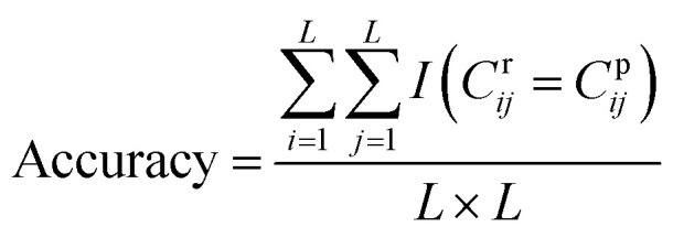
DGraphDTA constructs the protein map through Pconsc4, and the accuracy of the contact map will directly influence the final prediction result. Therefore, in order to figure out whether the contact map predicted by Pconsc4 is helpful to the prediction of affinity, an evaluation experiment was carried out. We searched for the 229 proteins of KIBA in the PDB database63 manually to find proteins which have complete structures corresponding to the given sequence, and there are 35 proteins meeting the requirements. In the 35 proteins, there are still some missing residues in their structures. Therefore, we only exported the actual contact map of the recorded residues using three thresholds (6 Å, 8 Å and 10 Å), and then extracted the contact map predicted by Pconsc4 with the corresponding positions for comparison using eqn (13):
 |
13 |
where L is the sequence length, Cr is the actual contact map, Cp is the predicted contact map, and I(x) is a function such that I(x) = 1 when the condition x is satisfied, otherwise I(x) = 0. The accuracy of the contact map predicted by Pconsc4 is shown in Table 11.
The accuracy of contact map predicted by Pconsc4.
| Threshold: 6 Å | Threshold: 8 Å | Threshold: 10 Å | |
|---|---|---|---|
| Accuracy | 98.3% | 98.4% | 96.8% |
The table illustrates that the contact map predicted by Pconsc4 is basically consistent with the actual contact map, which can reach an accuracy of 98% with a threshold of 8 Å. It also indicates that the contact map predicted by Pconsc4 can show the spatial structure of the protein to a certain extent, so it can be used in the prediction of affinity.
In addition, we used the actual contact map (with a threshold of 8 Å) and the contact map predicted from Pconsc4 to train two independent models to predict the affinity with DGraphDTA using the same training and test sets. There are 12 016 drug–target pairs in the training set and 2451 drug–target pairs in the test set that cover these 35 proteins in the KIBA dataset. The results are shown in Table 12. It can be seen from Table 12 that the predictions using the contact map predicted by Pconsc4 are basically the same as those using the actual contact maps. The result with Pconsc4 is slightly better than that with actual contact map. On the one hand, because the actual protein structure is more or less missing some amino records, the actual contact map obtained is only a part of the whole map, which may lose some structural information. On the other hand, Pconsc4 uses a combination of predictions with different thresholds for further analysis. The output contact map is not the result under a certain threshold, but a more comprehensive contact map. Whether using the contact map predicted by Pconsc4 or the actual contact map, the prediction performance of the training model has declined compared with the results using the whole training set, because the 12 016 drug–target pairs that can cover the 35 proteins in the training set are only a small part of the whole original data set (with 98 585 pairs in the training set).
Performances using the actual contact map and Pconsc4-predicted contact map.
| Contact map type | CI (std) | MSE (std) | Pearson (std) |
|---|---|---|---|
| Contact map (actual) | 0.863 | 0.228 | 0.810 |
| Contact map (Pconsc4) | 0.861 | 0.212 | 0.825 |
The residues of proteins have various properties, such as hydrophobicity, aromaticity, solubility, etc. These properties will be reflected by various non-bonded interactions such as hydrophobic forces and hydrogen bonds, and influence the binding of proteins. So this information cannot be ignored when binding with small molecules. In the sequence-based DTA prediction, if only the residue type is considered, the sequence will be regarded as a symbol string, and the important property will be ignored. In DGraphDTA, the information and the topological connection between residues will be convoluted and extracted by the GNN, so it can extract the spatial structure and attribute information of the protein, and represents it more comprehensively.
It is worth mentioning that many protein structure prediction methods have emerged, so with the further improvement of their accuracy, the performance of DGraphDTA will also be improved. At the same time, due to the limitation of our hardware environments, only three layers of GNN are explored. When there are better GPUs to explore more types of GNN (such as more layers), there may be a better prediction result. In addition, the speed of the method much depends on the speed of the sequence alignment and contact map prediction of Pconsc4. Therefore, when the processes of these two aspects are accelerated, the prediction will be more rapid. The code of DGraphDTA and the relevant data are freely available at: https://github.com/595693085/DGraphDTA.
4. Conclusions
DTA prediction is an important step in virtual screening of computer-aided drug design, which can accelerate the process of drug design. In order to improve the accuracy of prediction of DTA, the methods based on deep learning have been gradually proposed. In this paper, the graphs of molecule and protein are each constructed. Furthermore, two GNNs are used to obtain their representations. In order to solve the problem of the construction of the protein graph, the structure prediction method is introduced to obtain the contact map of the protein. A method called DGraphDTA combining both molecular graph and protein graph is proposed. On the one hand, the method proposed in this paper greatly improves the accuracy of DTA prediction. On the other hand, our novel method of using protein sequence to construct graphs also provides a robust protein descriptor in drug design.
Conflicts of interest
There are no conflicts to declare.
Supplementary Material
Acknowledgments
This research was funded by the National Key Research and Development Program of China (no. 2019YFD0900401) and Marine S&T Fund of Shandong Province for Pilot National Laboratory for Marine Science and Technology (Qingdao) (no. 2018SDKJ0402).
References
- Aminpour M. Montemagno C. Tuszynski J. A. Molecules. 2019;24:1693. doi: 10.3390/molecules24091693. [DOI] [PMC free article] [PubMed] [Google Scholar]
- Phillips J. C. Braun R. Wang W. Gumbart J. Tajkhorshid E. Villa E. Chipot C. Skeel R. D. Kale L. Schulten K. J. Comput. Chem. 2005;26:1781–1802. doi: 10.1002/jcc.20289. [DOI] [PMC free article] [PubMed] [Google Scholar]
- Van Der Spoel D. Lindahl E. Hess B. Groenhof G. Mark A. E. Berendsen H. J. C. J. Comput. Chem. 2005;26:1701–1718. doi: 10.1002/jcc.20291. [DOI] [PubMed] [Google Scholar]
- Salomon-Ferrer R. Case D. A. Walker R. C. Wiley Interdiscip. Rev.: Comput. Mol. Sci. 2013;3:198–210. [Google Scholar]
- Lang P. T. Brozell S. R. Mukherjee S. Pettersen E. F. Meng E. C. Thomas V. Rizzo R. C. Case D. A. James T. L. Kuntz I. D. Rna. 2009;15:1219–1230. doi: 10.1261/rna.1563609. [DOI] [PMC free article] [PubMed] [Google Scholar]
- Morris G. M. Huey R. Lindstrom W. Sanner M. F. Belew R. K. Goodsell D. S. Olson A. J. J. Comput. Chem. 2009;30:2785–2791. doi: 10.1002/jcc.21256. [DOI] [PMC free article] [PubMed] [Google Scholar]
- Hartshorn M. J. Verdonk M. L. Chessari G. Brewerton S. C. Mooij W. T. M. Mortenson P. N. Murray C. W. J. Med. Chem. 2007;50:726–741. doi: 10.1021/jm061277y. [DOI] [PubMed] [Google Scholar]
- Preuer K. Lewis R. P. I. Hochreiter S. Bender A. Bulusu K. C. Klambauer G. Bioinformatics. 2018;34:1538–1546. doi: 10.1093/bioinformatics/btx806. [DOI] [PMC free article] [PubMed] [Google Scholar]
- Mayr A. Klambauer G. Unterthiner T. Hochreiter S. Front. Environ. Sci. Eng. 2016;3:80. [Google Scholar]
- Council N. R. and others, Toxicity testing in the 21st century: a vision and a strategy, National Academies Press, 2007 [Google Scholar]
- Bashir M. Y., Muneer K., Mustafa R. and Rehman H. U., in 2019 15th International Conference on Emerging Technologies, ICET, 2019, pp. 1–6 [Google Scholar]
- Lenselink E. B. Ten Dijke N. Bongers B. Papadatos G. Van Vlijmen H. W. T. Kowalczyk W. IJzerman A. P. Van Westen G. J. P. J. Cheminf. 2017;9:1–14. doi: 10.1186/s13321-017-0232-0. [DOI] [PMC free article] [PubMed] [Google Scholar]
- Cortés-Ciriano I. Ain Q. U. Subramanian V. Lenselink E. B. Méndez-Lucio O. IJzerman A. P. Wohlfahrt G. Prusis P. Malliavin T. E. van Westen G. J. P. others Medchemcomm. 2015;6:24–50. doi: 10.1039/C4MD00216D. [DOI] [Google Scholar]
- Rifaioglu A. Sinoplu E. Atalay V. Martin M. Cetin-Atalay R. Dogan T. Chem. Sci. 2020;11:2531–2557. doi: 10.1039/C9SC03414E. [DOI] [PMC free article] [PubMed] [Google Scholar]
- Wen M. Zhang Z. Niu S. Sha H. Yang R. Yun Y. Lu H. J. Proteome Res. 2017;16:1401–1409. doi: 10.1021/acs.jproteome.6b00618. [DOI] [PubMed] [Google Scholar]
- Damale M. G. Patil R. B. Ansari S. A. Alkahtani H. M. Almehizia A. A. Shinde D. B. Arote R. Sangshetti J. RSC Adv. 2019;9:26176–26208. doi: 10.1039/C9RA03281A. [DOI] [PMC free article] [PubMed] [Google Scholar]
- Loo J. S. E. Emtage A. L. Murali L. Lee S. S. Kueh A. L. W. Alexander S. P. H. RSC Adv. 2019;9:15949–15956. doi: 10.1039/C9RA01095E. [DOI] [PMC free article] [PubMed] [Google Scholar]
- Jana S. Ganeshpurkar A. Singh S. K. RSC Adv. 2018;8:39477–39495. doi: 10.1039/C8RA08198K. [DOI] [PMC free article] [PubMed] [Google Scholar]
- Liu Y. Wu M. Miao C. Zhao P. Li X.-L. PLoS Comput. Biol. 2016;12:e1004760. doi: 10.1371/journal.pcbi.1004760. [DOI] [PMC free article] [PubMed] [Google Scholar]
- Nascimento A. C. A. Prudêncio R. B. C. Costa I. G. BMC Bioinf. 2016;17:46. doi: 10.1186/s12859-016-0890-3. [DOI] [PMC free article] [PubMed] [Google Scholar]
- Keum J. Nam H. PLoS One. 2017;12:e0171839. doi: 10.1371/journal.pone.0171839. [DOI] [PMC free article] [PubMed] [Google Scholar]
- Barbet J. Huclier-Markai S. Pharm. Stat. 2019;18:513–525. doi: 10.1002/pst.1943. [DOI] [PubMed] [Google Scholar]
- Yung-Chi C. Prusoff W. H. Biochem. Pharmacol. 1973;22:3099–3108. doi: 10.1016/0006-2952(73)90196-2. [DOI] [PubMed] [Google Scholar]
- Öztürk H. Özgür A. Ozkirimli E. Bioinformatics. 2018;34:i821–i829. doi: 10.1093/bioinformatics/bty593. [DOI] [PMC free article] [PubMed] [Google Scholar]
- Öztürk H., Ozkirimli E. and Özgür A., 2019, arXiv Prepr. arXiv:1902.04166
- Huang Y.-A. You Z.-H. Chen X. Curr. Protein Pept. Sci. 2018;19:468–478. doi: 10.2174/1389203718666161122103057. [DOI] [PubMed] [Google Scholar]
- Lee H. Kim W. Pharmaceutics. 2019;11:377. doi: 10.3390/pharmaceutics11080377. [DOI] [PMC free article] [PubMed] [Google Scholar]
- Rogers D. Hahn M. J. Chem. Inf. Model. 2010;50:742–754. doi: 10.1021/ci100050t. [DOI] [PubMed] [Google Scholar]
- Bender A. Mussa H. Y. Glen R. C. Reiling S. J. Chem. Inf. Comput. Sci. 2004;44:1708–1718. doi: 10.1021/ci0498719. [DOI] [PubMed] [Google Scholar]
- Durant J. L. Leland B. A. Henry D. R. Nourse J. G. J. Chem. Inf. Comput. Sci. 2002;42:1273–1280. doi: 10.1021/ci010132r. [DOI] [PubMed] [Google Scholar]
- Wu Z. Ramsundar B. Feinberg E. N. Gomes J. Geniesse C. Pappu A. S. Leswing K. Pande V. Chem. Sci. 2018;9:513–530. doi: 10.1039/C7SC02664A. [DOI] [PMC free article] [PubMed] [Google Scholar]
- Altae-Tran H. Ramsundar B. Pappu A. S. Pande V. ACS Cent. Sci. 2017;3:283–293. doi: 10.1021/acscentsci.6b00367. [DOI] [PMC free article] [PubMed] [Google Scholar]
- van Westen G. J. P. Swier R. F. Wegner J. K. IJzerman A. P. van Vlijmen H. W. T. Bender A. J. Cheminf. 2013;5:41. doi: 10.1186/1758-2946-5-41. [DOI] [PMC free article] [PubMed] [Google Scholar]
- Wang Y.-B. You Z.-H. Yang S. Yi H.-C. Chen Z.-H. Zheng K. BMC Med. Inf. Decis. Making. 2020;20:1–9. doi: 10.1186/s12911-019-1002-x. [DOI] [PMC free article] [PubMed] [Google Scholar]
- Kipf T. N. and Welling M., 2016, arXiv Prepr. arXiv:1609.02907
- Veličković P., Cucurull G., Casanova A., Romero A., Lio P. and Bengio Y., 2017, arXiv Prepr. arXiv:1710.10903
- Liu K. Sun X. Jia L. Ma J. Xing H. Wu J. Gao H. Sun Y. Boulnois F. Fan J. Int. J. Mol. Sci. 2019;20:3389. doi: 10.3390/ijms20143389. [DOI] [PMC free article] [PubMed] [Google Scholar]
- Kearnes S. McCloskey K. Berndl M. Pande V. Riley P. J. Comput.-Aided Mol. Des. 2016;30:595–608. doi: 10.1007/s10822-016-9938-8. [DOI] [PMC free article] [PubMed] [Google Scholar]
- Feng Q., Dueva E., Cherkasov A. and Ester M., 2018, arXiv Prepr. arXiv:1807.09741
- Nguyen T. Le H. Venkatesh S. bioRxiv. 2019:684662. [Google Scholar]
- Wu Q. Peng Z. Anishchenko I. Cong Q. Baker D. Yang J. Bioinformatics. 2020;36:41–48. doi: 10.1093/bioinformatics/btz477. [DOI] [PMC free article] [PubMed] [Google Scholar]
- Wang S. Sun S. Li Z. Zhang R. Xu J. PLoS Comput. Biol. 2017;13:e1005324. doi: 10.1371/journal.pcbi.1005324. [DOI] [PMC free article] [PubMed] [Google Scholar]
- Adhikari B. Hou J. Cheng J. Bioinformatics. 2017;34:1466–1472. doi: 10.1093/bioinformatics/btx781. [DOI] [PMC free article] [PubMed] [Google Scholar]
- Hanson J. Paliwal K. Litfin T. Yang Y. Zhou Y. Bioinformatics. 2018;34:4039–4045. doi: 10.1093/bioinformatics/bty481. [DOI] [PubMed] [Google Scholar]
- Liu Y. Palmedo P. Ye Q. Berger B. Peng J. Cell Syst. 2018;6:65–74. doi: 10.1016/j.cels.2017.11.014. [DOI] [PMC free article] [PubMed] [Google Scholar]
- Xiong D. Zeng J. Gong H. Bioinformatics. 2017;33:2675–2683. doi: 10.1093/bioinformatics/btx296. [DOI] [PubMed] [Google Scholar]
- Jones D. T. Singh T. Kosciolek T. Tetchner S. Bioinformatics. 2014;31:999–1006. doi: 10.1093/bioinformatics/btu791. [DOI] [PMC free article] [PubMed] [Google Scholar]
- Seemayer S. Gruber M. Söding J. Bioinformatics. 2014;30:3128–3130. doi: 10.1093/bioinformatics/btu500. [DOI] [PMC free article] [PubMed] [Google Scholar]
- Michel M. Menéndez Hurtado D. Elofsson A. Bioinformatics. 2019;35:2677–2679. doi: 10.1093/bioinformatics/bty1036. [DOI] [PubMed] [Google Scholar]
- Pahikkala T. Airola A. Pietilä S. Shakyawar S. Szwajda A. Tang J. Aittokallio T. Briefings Bioinf. 2014;16:325–337. doi: 10.1093/bib/bbu010. [DOI] [PMC free article] [PubMed] [Google Scholar]
- He T. Heidemeyer M. Ban F. Cherkasov A. Ester M. J. Cheminf. 2017;9:24. doi: 10.1186/s13321-017-0209-z. [DOI] [PMC free article] [PubMed] [Google Scholar]
- Ronneberger O., Fischer P. and Brox T., in International Conference on Medical image computing and computer-assisted intervention, 2015, pp. 234–241 [Google Scholar]
- cheol J. J. Lin X. Chen X.-W. IEEE/ACM Trans. Comput. Biol. Bioinf. 2010;8(2):308–315. doi: 10.1109/TCBB.2010.93. [DOI] [PubMed] [Google Scholar]
- Nishida K. Frith M. C. Nakai K. Nucleic Acids Res. 2008;37:939–944. doi: 10.1093/nar/gkn1019. [DOI] [PMC free article] [PubMed] [Google Scholar]
- Steinegger M. Meier M. Mirdita M. Voehringer H. Haunsberger S. J. Soeding J. bioRxiv. 2019:560029. doi: 10.1186/s12859-019-3019-7. [DOI] [PMC free article] [PubMed] [Google Scholar]
- Jones D. T. Buchan D. W. A. Cozzetto D. Pontil M. Bioinformatics. 2011;28:184–190. doi: 10.1093/bioinformatics/btr638. [DOI] [PubMed] [Google Scholar]
- Gönen M. Heller G. Biometrika. 2005;92:965–970. doi: 10.1093/biomet/92.4.965. [DOI] [Google Scholar]
- Allen D. M. Technometrics. 1971;13:469–475. doi: 10.1080/00401706.1971.10488811. [DOI] [Google Scholar]
- Benesty J., Chen J., Huang Y. and Cohen I., in Noise reduction in speech processing, Springer, 2009, pp. 1–4 [Google Scholar]
- Roy K. Chakraborty P. Mitra I. Ojha P. K. Kar S. Das R. N. J. Comput. Chem. 2013;34:1071–1082. doi: 10.1002/jcc.23231. [DOI] [PubMed] [Google Scholar]
- Smith T. F. Waterman M. S. J. Mol. Biol. 1981;147:195–197. doi: 10.1016/0022-2836(81)90087-5. [DOI] [PubMed] [Google Scholar]
- Kim S. Chen J. Cheng T. Gindulyte A. He J. He S. Li Q. Shoemaker B. A. Thiessen P. A. Yu B. others Nucleic Acids Res. 2018;47:D1102–D1109. doi: 10.1093/nar/gky1033. [DOI] [PMC free article] [PubMed] [Google Scholar]
- Berman H. M. Westbrook J. Feng Z. Gilliland G. Bhat T. N. Weissig H. Shindyalov I. N. Bourne P. E. Nucleic Acids Res. 2000;28:235–242. doi: 10.1093/nar/28.1.235. [DOI] [PMC free article] [PubMed] [Google Scholar]
- Lide D. R., CRC Handbook of Chemistry and Physics, Chemical Rubber Pub. Co., Boston, 1991, pp. 4–50 [Google Scholar]
- Sereda T. J. Mant C. T. Sönnichsen F. D. Hodges R. S. J. Chromatogr. A. 1994;676:139–153. doi: 10.1016/0021-9673(94)00371-8. [DOI] [PubMed] [Google Scholar]
- Monera O. D. Sereda T. J. Zhou N. E. Kay C. M. Hodges R. S. J. Pept. Sci. an Off. Publ. Eur. Pept. Soc. 1995;1:319–329. doi: 10.1002/psc.310010507. [DOI] [PubMed] [Google Scholar]


