

Abstract
Background
Emerging studies have investigated the contribution of food environment to obesity in the USA. However, the findings were inconsistent. Methodological explanations for the inconsistent findings included: (1) using individual store/restaurant exposure as food environment indicator, and (2) not accounting for non-stationarity assumption. This study aimed to describe the spatial distribution of obesity and examine the association between community food environment and obesity, and the variation of magnitude and direction of this association across the USA.
Methods
Data from 20 897 adults who participated in the REasons for Geographic and Racial Differences in Stroke study and completed baseline assessment between January 2003 and October 2007 were eligible in analysis. Hot Spot analysis was used to assess the spatial distribution of obesity. The association between community food environment and obesity and the variation of this association across the USA were examined using global ordinary least squares regression and local geographically weighted regression.
Results
Higher body mass index (BMI) clusters were more likely to locate in socioeconomically disadvantaged, rural, minority neighbourhoods with a smaller population size, while lower BMI clusters were more likely to appear in more affluent, urban neighbourhoods with a higher percentage of non-Hispanic white residences. There was an overall significant, inverse association between community food environment and obesity (β=−0.0210; p<0.0001). Moreover, the magnitude and direction of this association varied significantly across the US regions.
Conclusions
The findings underscored the need for geographically tailored public health interventions and policies to address unique local food environment issues to achieve maximum effects on obesity prevention.
INTRODUCTION
Obesity is a major public health problem in the USA owing to its rapidly increasing prevalence, substantial mortality and morbidity and growing healthcare costs.1 2 There is significant disparity in the geographical distribution of obesity across the USA. In particular, obesity is especially prevalent in rural areas and the Southern USA.3 4
Recent research has focused on understanding the contribution of community food environment, defined as the distribution of food sources, involving the number, type, location and accessibility of food outlets, to obesity and its disparities across the USA5 6 However, the findings from previous studies were inconsistent. Feng et al,7 Gamba et al8 and Cobb et al5 reviewed over 60 studies among US adults.5 7 8 Some studies found that access to healthful food outlets were inversely related to obesity, while a few studies found positive associations.9-14 Some studies found that access to unhealthful food outlets were positively correlated with obesity; however, others found null or even, negative associations.15-20
One major methodological issue with previous studies, which may help explain the inconsistent findings, is that most of the studies used limited food source measures, by only considering access to individual store/restaurant types. For instance, Oreskovic et al21 and Reitzel et al22 used fast food exposure as their sole measure of food environment.21 22 These limited measures may yield biased and inconsistent results due to not providing a complete picture of an individual’s food environment. Experts have suggested using food environment measures that combine multiple food outlet types (eg, index designed to capture the ratio of unhealthy to healthy food outlets) which can provide a more robust measure of the overall healthfulness of food environment. The other main methodological issue is applying a global regression model for the entire country which assumes that the relationship between food environment and obesity is invariant across space. However, empirical evidence has suggested that the association between food environment and obesity may vary geographically. For instance, a 2013 study in California found no association between food outlets within walking distance and obesity, while a similar study in 2014 in New Jersey found that densities of fast-food restaurants were positively associated with obesity.10 23
This study attempts to overcome these aforementioned methodological issues by using geospatial modelling techniques, in order to describe the spatial distribution of obesity, examining the relationship between community food environment and obesity, and investigating the variation of this relationship across the USA. It is hypothesised that obesity is linked to community food environment, and this relationship varies across the USA.
METHODS
Data source and study participants
Data for individuals were drawn from the REasons for Geographic And Racial Differences in Stroke (REGARDS) study, a national longitudinal cohort study of black and white community-dwelling residents aged 45 years and older to investigate the contributors to stroke in the USA.24 For our study, participants who completed baseline assessment during January 2003 and October 2007, with body weight and geocoded address were eligible. Individuals who did not have body weight (n=215) or geocoded address (n=11) were excluded from analysis. Furthermore, participants whose geocoded address could not match with 2000 census tract (n=2), did not have matched food environment data (n=78), and whose body mass index (BMI) were significant outliers (n=53) were excluded. Community food environment data were retrieved from the Centers for Disease Control and Prevention.25 Community data were drawn from Food Environment Atlas (2011), and Census of Population and Housing (2000).26 27 The census tract shapefiles (2000) were downloaded from the US Census Bureau.28
Variables
Community food environment
Modified Retail Food Environment Index (mRFEI) was used as community food environment indicator. The mRFEI represents the percentage of food retailers that were designated ‘healthy’—including supermarkets, larger grocery stores, supercenters and produce stores—out of the total number of food retailers within a given census tract. The mRFEI ranges from 0 to 100, with higher mRFEI scores indicating greater access to healthy food retailers in census tracts.25
Obesity
BMI (kg/m2) was used to measure obesity. BMI was calculated using height and weight measured during the REGARDS study home visit. Height was obtained using an 8-foot metal tape measure without shoes. Weight was measured using a standard 300 lb calibrated digital scale.24
Covariates
Sociodemographics
The following variables were included: age (years; continuous), sex (male vs female), race (white vs black), health insurance (yes vs no), marital status (single, married, divorced, widowed or other), education (less than high school, high school graduate, some college, or college graduate and above), annual household income (<20 000, 20 000–34 000, 35 000–74 000, ≥75 000 or refused), employment (employment for wage, self-employed, unemployed for ≥1 year, unemployed for <1 year, home maker, students, retired, unable to work or refused) and time lived in current address (years; continuous).
Lifestyle
These factors included exercise (none, 1–3 times/week or ≥4 times/week), watch television (TV)/video (none, 1–6hours/week, 1 hour/day, 2 hours/day, 3 hours/day or ≥4 hours/day), alcohol use (none, moderate (women: 0–7 drinks/week; men: 0–14 drinks/week) or heavy (women: >7 drinks/week; men: >14 drinks/week)) and smoking (none, past or current).
Community features
Six factors were included1: percentage of county residents that was non-Hispanic white (2008),2 percentage of county residents that was non-Hispanic black (2008)3, county median household income (2008),4 county poverty rate (2008),5 census-tract population size (2000) and6 Rural–Urban Commuting Area Code (RUCA) (2000). RUCA codes were categorised and coded as 1=urban, 2=large rural city/town, 3=small rural town and 4=isolated small rural town, according to Categorization A by the University of Washington Rural Health Research Center.29
Data analysis
The spatial modelling was implemented using ArcGIS 10.4 (ESRI, Redlands, California). The REGARDS data and other community data were integrated and imported into ArcMap to prepare for analysis. First, Hot Spot analysis (Getis-Ord Gi*) of BMI was conducted to describe the geospatial distribution of obesity across the USA. Hot Spot analysis identifies statistically significant clusters of high or low value of a phenomenon of interest (eg, BMI) by evaluating each feature (eg, individual) in context of neighbouring features and against all features in the dataset.30 A hot spot is a feature with a high value surrounded by other features with high values, and a cold spot is a feature with a low value surrounded by other features with low values.31 Euclidean distance (the straight-line distance between two points) option was chosen to measure the distance between two individuals, and inverse distance option was used to conceptualise spatial relationship. False discovery rate correction was applied to account for both multiple testing and spatial dependence. Significance of local clustering was based on a p value <0.05.
Second, ordinary least squares (OLS) linear regression was conducted to examine the correlation between mRFEI and BMI. Coefficient, SEs and p value were reported. The performance of the model was evaluated by corrected Akaike Information Criterion (AICc) and spatial autocorrelation (Moran’s I) on regression residual.32 The Moran’s I index values ranged from −1 (negative autocorrelation) to +1 (positive autocorrelation). Significance of the spatial autocorrelation was based on a p value <0.05. A non-significant Moran’s I on the OLS model regression residual indicates that the model is well-specified; that is, the model includes key predictors for the dependent variable.32 Third, local geographically weighted regression (GWR) was conducted to estimate the possible variations of the association between mRFEI and BMI across study areas. GWR is a local form of linear regression used to model spatially varying relationships; that is, a separate equation and local parameter for each individual in the analysis was generated using a ‘local’ subset of the data falling within the bandwidth of the target individual.33 An adaptive kernel type with AICc estimated bandwidth was used to calibrate the model in order to account for spatial structure. The performance of the model was evaluated by R2, AICc and Moran’s I. If the AICc of the GWR model is more than 3 lower than that of the OLS model, it signifies the benefits of moving from a global model to a local regression model. A non-significant Moran’s I indicates the model was properly specified. A raster surface, based on the regression coefficient of mRFEI from the GWR model, was created to visually present the variation of the relationship between mRFEI and BMI across the study areas.
The statistical analysis was implemented using SAS V.9.4 for Windows (SAS Institute). Descriptive analyses were conducted using PROC UNIVARIATE and PROC FREQ procedures. Means and standard deviations (for continuous variables) and percentages (for categorical variables) were calculated. The individual and community characteristics were compared among the BMI clustering groups using PROC (procedure) FREQ (freqency), PROC ANOVA (analysis of variance), and PROC NPAR1WAY (nonparametric tests for location and scale differences across a one-way classification) procedures as appropriate. The statistical significance, alpha, level was set at 0.05, two-tailed.
RESULTS
Descriptive analysis
A total of 20 897 participants from the contiguous united states (including 48 contiguous states and Washington, DC) were included in analysis. The participants’ individual characteristics and their community features are summarised in table 1. The mean age of the participants was 65 years, about half were retired, about half having an income >$35 000 and slightly more than half were women. About two-thirds of the participants were white, married and reported greater than high school education. Almost all participants had health insurance. In addition, the majority were not current smokers or alcohol users, exercised ≥1 time/week and watched TV/video ≥1 hour/day. Nearly 80% lived in urban areas for an average of 29 years at their current residence. The mean BMI was 28.96 kg/m2, with about 38% classified as overweight (25 kg/m2 ≤BMI <30kg/m2) and 36% as obese (BMI ≥30 kg/m2).
Table 1.
Summary of individual and community characteristics of the REasons for Geographic and Racial Differences in Stroke (REGARDS) study participants (n=20 897)
| Characteristics | REGARDS participants |
|---|---|
| Sociodemographics | |
| Age, year, mean (SD) | 64.88 (9.26) |
| Male, % (n) | 44.22 (9241) |
| White, % (n) | 66.71 (13 941) |
| Education, % (n) | |
| Less than high school | 9.58 (2002) |
| High school graduate | 25.52 (5331) |
| Some college | 27.32 (5707) |
| College graduate and above | 37.57 (7849) |
| Relationship, % (n) | |
| Single | 5.11 (1068) |
| Married | 61.74 (12901) |
| Divorced | 13.89 (2902) |
| Widowed | 17.41 (3638) |
| Other | 1.86 (388) |
| Annual household income, % (n) | |
| <20 000 | 15.63 (3266) |
| 20 000–34 000 | 24.09 (5034) |
| 35 000–74 000 | 31.39 (6559) |
| ≥75 000 | 17.18 (3590) |
| Refused | 11.71 (2448) |
| Employment, % (n) | |
| Employed for wages | 27.09 (3565) |
| Self-employed | 9.00 (1184) |
| Unemployed for ≥1 year | 1.47 (194) |
| Unemployed for <1 year | 1.48 (195) |
| Home maker | 6.08 (800) |
| Student | 0.19 (25) |
| Retired | 47.72 (6279) |
| Unable to work | 6.95 (914) |
| Refused | 0.02 (3) |
| Health insured, % (n) | 93.95 (19 620) |
| Time lived in current address, year, mean (SD) | 28.63 (20.62) |
| mRFEI, mean (SD) | 10.92 (10.19) |
| BMI, kg/m2, mean (SD) | 28.96 (5.90) |
| Overweight (25 kg/m2 ≤BMI <30 kg/m2), % (n) | 37.91 (7923) |
| Obese (BMI ≥30 kg/m2), % (n) | 36.17 (7558) |
| Life style | |
| Exercise, % (n) | |
| None | 32.50 (6701) |
| 1–3 times/week | 36.91 (7609) |
| ≥4 times/week | 30.59 (6307) |
| Watch TV/video, % (n) | |
| None | 0.76 (156) |
| 1–6 hours/week | 12.69 (2616) |
| 1 hour/day | 6.80 (1401) |
| 2 hours/day | 22.55 (4648) |
| 3 hours/day | 27.16 (5599) |
| ≥4 hours/day | 30.05 (6195) |
| Smoking,* % (n) | |
| Never | 45.23 (9417) |
| Past | 41.12 (8562) |
| Current | 13.65 (2842) |
| Alcohol use,† % (n) | |
| None | 59.64 (12 463) |
| Moderate | 35.93 (7508) |
| Heavy | 4.43 (926) |
| Community features | |
| Percentage of non-Hispanic white,‡ mean (SD) | 59.53 (18.95) |
| Percentage of non-Hispanic black,‡ mean (SD) | 26.62 (18.34) |
| Median household income,‡ $, mean (SD) | 48 182.49 (11 932.72) |
| Poverty rate,‡ mean (SD) | 15.92 (5.41) |
| Tract population§ mean (SD) | 5081.58 (2387.90) |
| RUCA code,§ % (n) | |
| Urban | 76.99 (16 089) |
| Large rural | 12.61 (2635) |
| Small rural | 6.98 (1459) |
| Isolated small rural | 3.42 (714) |
Never smoker is defined as an adult who has smoked <100 cigarettes per lifetime and not smoking at the time of interview; past smoker is defined as an adult who has smoked at least 100 cigarettes in his or her lifetime but who had quit smoking at the time of interview; current smoker is defined as an adult who has smoked 100 cigarettes in his or her lifetime and who currently smokes cigarettes.
Moderate alcohol use is defined as 0–7 drinks/week for women and 0–14 drinks/week for men; heavy alcohol use is defined as having >7 drinks/week for women and >14 drinks/week for men.
County-level data.
Census-tract-level data. Refer to online supplementary appendix for more details of RUCA code categories.
BMI, body mass index; mRFEI, modified retail food environment index; RUCA, Rural–Urban Commuting Area Code; TV, television.
Hot spot analysis
Figure 1 displays the result of Hot Spot analysis of BMI. Black points denote high BMI clusters, whereas grey points denote low BMI clusters. The higher BMI clusters (hot spot; black points) were found in Eastern Virginia, Northern Ohio, Eastern Michigan, Northern Indiana, Southwestern Georgia, Northwestern Florida and Southern Louisiana. The lower BMI cluster (cold spot; grey points) appeared in Northwestern Washington, Central Northern Colorado, Central Eastern Tennessee, Western North Carolina, New Jersey, Southern New York, Connecticut and Massachusetts.
Figure 1.
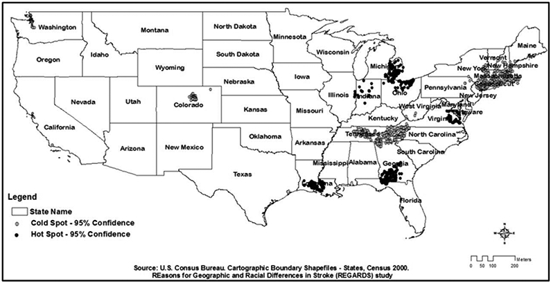
Hot Spot Analysis (Getis-Ord Gi*) for BMI among the REGARDS study participants across the USA (n=20897). Black (hot spot) indicates the clusters of participants with significantly higher BMI, comparing to all the participants across the study areas. The significance of local clustering was based on a p value <0.05. BMI, body mass index; REGARDS, Reasons for Geographic And Racial Differences in Stroke.
Table 2 shows the results of comparing participant characteristics and community features among BMI clusters. Participants in the higher BMI clusters were more likely to be younger age, black, not retired, not married, without health insurance, current smokers, non-alcohol user, not have a college degree, have an annual household income of <$35 000, exercise <4 times/week, watch TV/video ≥4 hours/day and reside longer in their current address, compared with those in lower BMI clusters or non-clustering areas. Moreover, higher BMI clusters were more likely to appear in neighbourhoods with a higher percentage of non-Hispanic black residents, a lower median household income, a higher poverty rate and a smaller population size.
Table 2.
Comparing individual and community characteristics among different BMI clusters
| Variables | Clusters |
|||
|---|---|---|---|---|
| Lower BMI (n=1187) |
Higher BMI (n=1630) |
Non-clustering (n=18 080) |
P values | |
| Sociodemographics | ||||
| Age, year, mean (SD) | 65.59 (8.81) | 64.09 (9.01) | 64.90 (9.31) | <0.0001 |
| Male, % (n) | 46.08 (547) | 44.66 (728) | 44.06 (7966) | 0.3703 |
| White, % (n) | 74.22 (881) | 51.96 (847) | 67.55 (12 213) | <0.0001 |
| Education, % (n) | <0.0001 | |||
| Less than high school | 6.57 (78) | 11.72 (191) | 9.59 (1733) | |
| High school graduate | 22.33 (265) | 31.25 (509) | 25.21 (4557) | |
| Some college | 25.44 (302) | 27.56 (449) | 27.42 (4956) | |
| College graduate and above | 45.66 (542) | 29.47 (480) | 37.77 (6827) | |
| Relationship, % (n) | <0.0001 | |||
| Single | 6.40 (76) | 6.56 (107) | 4.89 (885) | |
| Married | 61.33 (728) | 56.63 (923) | 62.22 (11 250) | |
| Divorced | 14.32 (170) | 16.81 (274) | 13.60 (2458) | |
| Widowed | 15.75 (187) | 17.73 (289) | 17.49 (3162) | |
| Other | 2.19 (26) | 2.27 (37) | 1.80 (325) | |
| Income, % (n) | <0.0001 | |||
| <20 000 | 11.46 (136) | 19.94 (325) | 15.51 (2805) | |
| 20 000–34 000 | 24.01 (285) | 26.01 (424) | 23.92 (4325) | |
| 35 000–74 000 | 34.12 (405) | 27.79 (453) | 31.53 (5701) | |
| ≥75 000 | 18.96 (225) | 14.85 (242) | 17.27 (3123) | |
| Refused | 11.46 (136) | 11.41 (186) | 11.76 (2126) | |
| Employment, % (n) | 0.0763 | |||
| Employed for wages | 24.68 (156) | 30.44 (274) | 26.96 (3135) | |
| Self-employed | 9.81 (62) | 8.11 (73) | 9.02 (1049) | |
| Unemployed for ≥1 year | 1.58 (10) | 1.67 (15) | 1.45 (169) | |
| Unemployed for <1 year | 1.58 (10) | 1.67 (15) | 1.46 (170) | |
| Home maker | 5.54 (35) | 5.22 (47) | 6.18 (718) | |
| Student | 0.63 (4) | 0.33 (3) | 0.15 (18) | |
| Retired | 51.42 (325) | 45.44 (409) | 47.69 (5545) | |
| Unable to work | 4.75 (30) | 7.11 (64) | 7.05 (820) | |
| Refused | 0.00 (0) | 0.00 (0) | 0.03 (3) | |
| Health insured, % (n) | 96.21 (1141) | 92.51 (1506) | 93.93 (16 973) | 0.0002 |
| Time in current address, year, mean (SD) | 26.30 (20.06) | 32.91 (20.66) | 28.40 (20.60) | <0.0001 |
| mRFEI, mean (SD) | 10.30 (9.54) | 10.mRFEI.73) | 11.02 (10.27) | 0.0027 |
| BMI, mean (SD) | 27.91 (5.38) | 29.81 (6.35) | 28.96 (5.88) | <0.0001 |
| Obese, % (n) | 28.98 (344) | 40.98 (668) | 36.21 (6546) | <0.0001 |
| Overweight/obese | 68.41 (812) | 77.30 (1260) | 74.16 (13 409) | <0.0001 |
| Life style | ||||
| Exercise, % (n) | 0.0296 | |||
| None | 30.32 (356) | 34.33 (551) | 32.48 (5794) | |
| 1–3 times/week | 37.73 (443) | 38.26 (614) | 36.73 (6552) | |
| ≥4 times/week | 31.94 (375) | 27.41 (440) | 30.79 (5492) | |
| Watch TV/video, % (n) | <0.0001 | |||
| None | 1.02 (12) | 0.63 (10) | 0.75 (134) | |
| 1–6 hours/week | 14.66 (173) | 12.34 (197) | 12.59 (2246) | |
| 1 hour/day | 6.61 (78) | 6.39 (102) | 6.84 (1221) | |
| 2 hours/day | 26.61 (314) | 19.97 (319) | 22.51 (4015) | |
| 3 hours/day | 26.95 (318) | 26.11 (417) | 27.27 (4864) | |
| 4+ hours/day | 24.15 (285) | 34.56 (552) | 30.04 (5358) | |
| Smoking,* % (n) | 0.0004 | |||
| Never | 45.23 (536) | 41.06 (666) | 45.60 (8215) | |
| Past | 40.42 (479) | 42.23 (685) | 41.07 (7398) | |
| Current | 14.35 (170) | 16.71 (271) | 13.33 (2401) | |
| Alcohol use,† % (n) | 0.0030 | |||
| None | 55.10 (654) | 60.86 (992) | 59.83 (10 817) | |
| Moderate | 41.11 (488) | 35.09 (572) | 35.66 (6448) | |
| Heavy | 3.79 (45) | 4.05 (66) | 4.51 (815) | |
| Community features | ||||
| Per cent of non-Hispanic | 70.78 (21.23) | 59.84 (15.12) | 58.76 (18.87) | <0.0001 |
| White,‡ mean (SD) | ||||
| Per cent of non-Hispanic | 11.84 (10.06) | 32.88 (15.43) | 27.03 (18.51) | <0.0001 |
| Black,‡ mean (SD) | ||||
| Median household income,‡ $, mean (SD) | 54 722.68 (14 947.37) | 44 277.76 (9198.25) | 48 105.15 (11751.90) | <0.0001 |
| Poverty rate,‡ mean (SD) | 13.40 (4.74) | 18.22 (5.16) | 15.88 (5.39) | <0.0001 |
| Tract population,§ mean (SD) | 5077.94 (2596.33) | 4143.63 (1687.93) | 5166.38 (2409.38) | <0.0001 |
| RUCA code,§ % (n) | <0.0001 | |||
| Urban | 87.53 (1039) | 81.17 (1323) | 75.92 (13 727) | |
| Large rural | 6.74 (80) | 12.70 (207) | 12.99 (2348) | |
| Small rural | 3.12 (37) | 4.85 (79) | 7.43 (1343) | |
| Isolated small rural | 2.61 (31) | 1.29 (21) | 3.66 (662) | |
Never smoker is defined as an adult who has smoked <100 cigarettes per lifetime and not smoking at the time of interview; past smoker is defined as an adult who has smoked at least 100 cigarettes in his or her lifetime but who had quit smoking at the time of interview; current smoker is defined an adults who has smoked 100 cigarettes in his or her lifetime and who currently smokes cigarettes.
Moderate alcohol use is defined as 0–7 drinks/week for women and 0–14 drinks/week for men; heavy alcohol use is defined as having >7 drinks/week for women and >14 drinks/week for men.
County-level data.
Census-tract-level data. Refer to online supplementary appendix for more details of RUCA code categories.
BMI, body mass index; mRFEI, modified retail food environment index; RUCA, Rural–Urban Commuting Area Code; TV, television.
Global and local regression analysis
The global OLS regression showed that mRFEI was significantly, negatively associated with BMI; that is, when mRFEI increased, participants’ BMI reduced (β= −0.0210, SE = 0.0040; p<0.0001). Spatial autocorrelation on regression residuals was detected (Moran’s I index=0.0041; p<0.0001). The relationship between mRFEI and BMI was not statistically significant after adjusting for sociodemographic, lifestyle and community feature covariates. Local GWR, using 992 neighbours to calibrate each local regression equation yielded optimal results. Compared with global regression, local modelling was associated with both a lower AICc (OLS: 133492.56; GWR: 133418.92; almost 74 points less) and a suppression of spatial autocorrelation in standardised residuals (Moran’s I index=−0.0031; p=0.3427).
Figure 2 depicts the spatial variations of the relationship between mRFEI and BMI across the USA. Darker areas indicate stronger, inverse relationship between mRFEI and BMI, whereas lighter areas indicate stronger, positive relations. Specifically, the results showed that greater access to healthy food outlets was strongly related to lower BMI in, for instance, Northern California, Central Texas, Montgomery area of Mississippi, Avoyelles area of Louisiana, Northern Alabama, Northwestern and Southeastern Georgia Laurens and Lancaster areas of South Carolina, Franklin area of North Carolina, Southeastern West Virginia and Western Virginia (darker areas). Greater access to healthful food outlets was significantly associated with higher BMI in, for instance, merging areas of Pennsylvania, Maryland, Washington DC, Delaware and Virginia; merging areas of Indiana, Ohio and Kentucky, Northeastern Arkansas, Southeastern North Carolina, Central Georgia, Northeastern Texas and Centeral Nevada (lighter areas).
Figure 2.
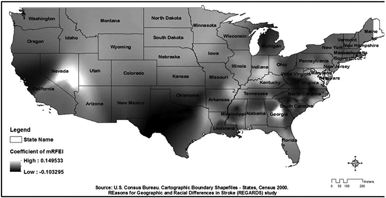
Spatial variation in the coefficient of mRFEI for the relationship between mRFEI and BMI among the REGARDS study participants (n=20897). A raster surface map, based on the regression coefficient of mRFEI from the geographically weighted regression model, presented the spatial variations of the relationship between mRFEI and BMI across the study areas. BMI, body mass index; mRFEI, modified Retail Food Environment Index; REGARDS, Reasons for Geographic and Racial Differences in Stroke.
DISCUSSION
The Hot Spot analysis supports previous reports of uneven distribution of obesity prevalence in the USA. Le et al study reported that obesity prevalence was higher in the South and North Central regions of the USA.4 Our study results echoed these findings. Befort et al study observed that obesity prevalence was lower among urban adults compared with rural adults.34 Our study found that lower BMI clusters were more likely to appear in relatively more affluent, urban areas. Moreover, our study emphasised the findings from recent nationwide studies that higher obesity prevalence was more likely to be located in socioeconomically disadvantaged, minority neighbourhoods with smaller population sizes.35 36 This suggests that global regression modelling for characterising obesity lacks the spatial resolution to accurately define hot spots of obesity; therefore, our GWR modelling approach is necessary to sufficiently highlight these geographical disparities. Moreover, the BMI clusters did not follow political boundaries (eg, state or county boundaries). For instance, one high BMI cluster extends egross the borders of Michigan and Ohio, and one low BMI cluster extends across the borders of New York, Massachusetts and Connecticut. These findings suggest that collaborations aimed at building regional/local networks might provide better resource alignment and more effective initiatives to prevent obesity at these specific places.
The finding from the global regression showed that greater access to healthy food outlets was significantly related to lower BMI which supports the findings of previous research. For instance, Morland and Evenson examining the association between access to food outlets and obesity in the Southern region of the USA found that areas with more supermarkets had lower obesity prevalence while areas with more small grocery stores or fast food restaurants had higher prevalence.11 Future studies should explore potential threshold and saturation effects of healthful food outlet exposure on obesity which will provide valuable guidance for future city planning or community zoning policies in food environment development and planning to yield optimal effects in reducing obesity.
The result of the local regression showed that there was variation in the relationship between food environment and obesity cross the USA which support our hypothesis. These findings also provide a potential explanation for the inconsistent findings from previous studies. For instance, in this study, we found relatively stronger and inverse relations between access to healthy food outlets and obesity in Northern California, while the relations in the southern areas of California were weaker and some were positive. This echoes the inconsistent findings from previous studies conducted in California. A study (2013) conducted among 97 678 participants in California found non-significant relationship between food outlets near home and BMI, while another study (2013) in Northern California area found that more healthful food environments were associated with lower risk of obesity.10 37
The relationship between food environment and obesity varies across the USA which demonstrates the need for developing geographically tailored programmes and policies to prevent obesity. Also, local programmes/policies may vary their efforts on modifying food environment in response to the variation of the food environment-obesity relationship across regions. For example, in regions where greater access to healthy food outlets is strongly associated with lower BMI, more effort should be spent improving access to healthy food than in regions where this association does not hold. Future studies are needed to confirm the findings from this study and examine the factors that contributed to such variations across the USA.
There are several strengths of this study. First, using local GWR modelling allows us to account for spatial heterogeneity in the relationship between community food environment and obesity across the USA. Second, mRFEI is a standardised composite measure that gives us a comprehensive picture of food environment that can be compared across studies. Third, keeping the spatial analysis at individual level helped avoid the potential bias introduced by analysis at the level of geographical boundaries (eg, at county level, at state level), as such boundaries are typically arbitegry and modifiable, especially when it is uncertain about the actual geographical areas that exert contextual influences on the relationship between food environment and obesity. Fourth, BMI was calculated based on the height and weight measured with a standardised protocol which prevented the potential bias introduced by using self-reported data.4 Lastly, using a large and geographically diverse sample allowed us to yield precise estimates.
Several limitations also should be noted. First, the cross-sectional design precluded drawing causal relationship between community food environment and obesity. Future experimental and longitudinal studies are needed to extend the findings from the current study. Second, the external validity of this study is limited. The participants were recruited using mail and telephone contacts which might preclude certain populations, especially in rural areas. Blacks and persons living in the eight southern ‘Stroke Belt’ states were oversampled.38 Moreover, the study only included mid-aged and older-age white and black residents which limited the capability to extend the findings to other age and racial/ethnic populations.
CONCLUSION
This study found that there was a significant and inverse relation between community food environment and obesity among US adults. More importantly, this relationship varied across the country. The findings from this study further emphasised the importance of accounting for spatial variations in future investigations on this topic and suggested the needs of geographically tailored public health policies and interventions to address issues unique to regional areas in order to achieve efficacious obesity prevention. Future studies examining the mechanisms underlying the relationship between the community food environment exposure and obesity outcome are warranted.
Supplementary Material
What is already known on this subject.
There is significant disparity in terms of geographical distribution of obesity across the USA and emerging interest in investigating the contribution of community food environment to the obesity epidemic and its disparity among the US population. However, the findings of the relationship between community food environment and obesity from previous studies were inconsistent.
What this study adds.
The innovation of this study is that it incorporated the non-stationarity assumption to investigate the variation of this relationship between community food environment and obesity across the US regions.
This nationwide study using local geographically weighted regression found that there was a significant and inverse relation between community food environment and obesity among US adults. More importantly, the magnitude and direction of this association varied significantly across the US regions.
The findings from this study explain the inconsistent findings from previous studies, extend our current understanding of the relationship between community food environment and obesity and its geographical disparity in the USA and provide evidence of the need of geographically tailored public health policies and interventions to address food environment issues unique to regional areas to achieve efficacious obesity prevention.
Acknowledgements
We thank the REGARDS research project (U01 NS041588) and The Mid-South Transdisciplinary Collaborative Center for Health Disparities Research (U54MD008176).
Footnotes
Competing interests None declared.
Ethics approval Permission and approval were obtained from the REGARDS study executive committee and the University of Alabama at Birmingham Institutional Review Board, respectively, to conduct this study.
REFERENCES
- 1.Singh GK, Siahpush M, Hiatt RA, et al. Dramatic increases in obesity and overweight prevalence and body mass index among ethnic-immigrant and social class groups in the United States, 1976-2008. J Community Health 2011;36:94–110. [DOI] [PMC free article] [PubMed] [Google Scholar]
- 2.Prevention. CfDCa. Overweight & Obesity. 2018. https://www.cdc.gov/obesity/index.html (updated 29 Nov 2017). [Google Scholar]
- 3.Myers CA, Slack T, Martin CK, et al. Regional disparities in obesity prevalence in the United States: A spatial regime analysis. Obesity 2015;23 481–7. [DOI] [PMC free article] [PubMed] [Google Scholar]
- 4.Le A, Judd SE, Allison DB, et al. The geographic distribution of obesity in the US and the potential regional differences in misreporting of obesity. Obesity 2014;22 300–6. [DOI] [PMC free article] [PubMed] [Google Scholar]
- 5.Cobb LK, Appel LJ, Franco M, et al. The relationship of the local food environment with obesity: A systematic review of methods, study quality, and results. Obesity 2015;23 1331–44. [DOI] [PMC free article] [PubMed] [Google Scholar]
- 6.Glanz K, Sallis JF, Saelens BE, et al. Healthy nutrition environments: concepts and measures. Am J Health Promot 2005;19:330–3. [DOI] [PubMed] [Google Scholar]
- 7.Feng J, Glass TA, Curriero FC, et al. The built environment and obesity: a systematic review of the epidemiologic evidence. Health Place 2010;16:175–90. [DOI] [PubMed] [Google Scholar]
- 8.Gamba RJ, Schuchter J, Rutt C, et al. Measuring the food environment and its effects on obesity in the United States: a systematic review of methods and results. J Community Health 2015;40:464–75. [DOI] [PubMed] [Google Scholar]
- 9.Ford PB, Dzewaltowski DA. Limited supermarket availability is not associated with obesity risk among participants in the Kansas WIC Program. Obesity 2010;18:1944–51. [DOI] [PubMed] [Google Scholar]
- 10.Hattori A, An R, Sturm R. Neighborhood food outlets, diet, and obesity among California adults, 2007 and 2009. Prev Chronic Dis 2013;10:E35. [DOI] [PMC free article] [PubMed] [Google Scholar]
- 11.Morland KB, Evenson KR. Obesity prevalence and the local food environment. Health Place 2009;15:491–5. [DOI] [PMC free article] [PubMed] [Google Scholar]
- 12.Gantner LA, Olson CM, Frongillo EA. Relationship of food availability and accessibility to women’s body weights in rural upstate New York. J Hunger Environ Nutr 2013;8:490–505. [Google Scholar]
- 13.Inagami S, Cohen DA, Brown AF, et al. Body mass index, neighborhood fast food and restaurant concentration, and car ownership. J Urban Health 2009;86:683–95. [DOI] [PMC free article] [PubMed] [Google Scholar]
- 14.Gibson DM. The neighborhood food environment and adult weight status: estimates from longitudinal data. Am J Public Health 2011;101:71–8. [DOI] [PMC free article] [PubMed] [Google Scholar]
- 15.Kumar S, Quinn SC, Kriska AM, et al. "Food is directed to the area": African Americans’ perceptions of the neighborhood nutrition environment in Pittsburgh. Health Place 2011;17:370–8. [DOI] [PMC free article] [PubMed] [Google Scholar]
- 16.Zenk SN, Lachance LL, Schulz AJ, et al. Neighborhood retail food environment and fruit and vegetable intake in a multiethnic urban population. Am J Health Promot 2009;23 255–64. [DOI] [PMC free article] [PubMed] [Google Scholar]
- 17.Bodor JN, Rice JC, Farley TA, et al. The association between obesity and urban food environments. J Urban Health 2010;87:771–81. [DOI] [PMC free article] [PubMed] [Google Scholar]
- 18.Mejia N, Lightstone AS, Basurto-Davila R, et al. Diet, and obesity among los angeles county adults, 2011. Preventing chronic disease 2015;12:E143. [DOI] [PMC free article] [PubMed] [Google Scholar]
- 19.Moore LV, Diez Roux AV, Nettleton JA, et al. Fast-food consumption, diet quality, and neighborhood exposure to fast food: the multi-ethnic study of atherosclerosis. Am J Epidemiol 2009;170 29–36. [DOI] [PMC free article] [PubMed] [Google Scholar]
- 20.Li F, Harmer P, Cardinal BJ, et al. Built environment and 1-year change in weight and waist circumference in middle-aged and older adults: Portland neighborhood environment and health study. Am J Epidemiol 2009;169:401–8. [DOI] [PMC free article] [PubMed] [Google Scholar]
- 21.Oreskovic NM, Winickoff JP, Kuhlthau KA, et al. Obesity and the built environment among Massachusetts children. Clin Pediatr 2009;48:904–12. [Google Scholar]
- 22.Reitzel LR, Regan SD, Nguyen N, et al. Density and proximity of fast food restaurants and body mass index among African Americans. Am J Public Health 2014;104:110–6. [DOI] [PMC free article] [PubMed] [Google Scholar]
- 23.Pruchno R, Wilson-Genderson M, Gupta AK. Neighborhood food environment and obesity in community-dwelling older adults: individual and neighborhood effects. Am J Public Health 2014;104:924–9. [DOI] [PMC free article] [PubMed] [Google Scholar]
- 24.Howard VJ, Cushman M, Pulley L, et al. The reasons for geographic and racial differences in stroke study: objectives and design. Neuroepidemiology 2005;25:135–43. [DOI] [PubMed] [Google Scholar]
- 25.Prevention CfDCa. Census tract level state maps of the Modified Retail Food Environment Index (mRFEI). Promotion NCfCDPaH. Ed. 2011. [Google Scholar]
- 26.Economic Research Service (ERS) USDoAU. Data access and documentation downloads. 2015. https://www.ers.usda.gov/data-products/food-environment-atlas/data-access-and-documentation-downloads/ (updated 19 Mar 2015). [Google Scholar]
- 27.Bureau USC. census of population and housing. 2018. https://www.census.gov/prod/www/decennial.html (updated 02 May 2018). [Google Scholar]
- 28.Bureau USC. cartographic boundary shapefiles. 2018. https://www.census.gov/geo/maps-data/data/tiger-cart-boundary.html (updated 09 Apr 2018). [Google Scholar]
- 29.University of Washington RHRC. RUCA Data: Using RUCA Data. 2017. http://depts.washington.edu/uwruca/ruca-uses.php (cited 04 Sep 2017). [Google Scholar]
- 30.Ord JK, Getis A. Local spatial autocorrelation statistics: distributional issues and an application. Geogr Anal 1995;27:286–306. [Google Scholar]
- 31.Pro A How hot spot analysis (Getis-Ord Gi*) works. 2017. http://pro.arcgis.com/en/pro-app/tool-reference/spatial-statistics/h-how-hot-spot-analysis-getis-ord-gi-spatial-stati.htm [Google Scholar]
- 32.ESRI. Spatial autocorrelation (Global Moran’s I): ESRI. 2017. http://pro.arcgis.com/en/pro-app/tool-reference/spatial-statistics/spatial-autocorrelation.htm [Google Scholar]
- 33.ESRI. Geographically Weighted Regression (GWR). 2017. 10.3/tools/spatial-statistics-toolbox/geographically-weighted-regression.htm [DOI] [Google Scholar]
- 34.Befort CA, Nazir N, Perri MG. Prevalence of obesity among adults from rural and urban areas of the United States: findings from NHANES (2005-2008). J Rural Health 2012;28:392–7. [DOI] [PMC free article] [PubMed] [Google Scholar]
- 35.Slack T, Myers CA, Martin CK, et al. The geographic concentration of US adult obesity prevalence and associated social, economic, and environmental factors. Obesity 2014;22:868–74. [DOI] [PubMed] [Google Scholar]
- 36.Singleton CR, Affuso O, Sen B. Decomposing racial disparities in obesity prevalence: Variations in retail food environment. Am J Prev Med 2016;50:365–72. [DOI] [PMC free article] [PubMed] [Google Scholar]
- 37.Jones-Smith JC, Karter AJ, Warton EM, et al. Obesity and the food environment: income and ethnicity differences among people with diabetes: the Diabetes Study of Northern California (DISTANCE). Diabetes Care 2013;36:2697–705. [DOI] [PMC free article] [PubMed] [Google Scholar]
- 38.Howard G, Howard VJ, Katholi C, et al. Decline in US stroke mortality: an analysis of temporal patterns by sex, race, and geographic region. Stroke 2001;32:2213–20. [DOI] [PubMed] [Google Scholar]
Associated Data
This section collects any data citations, data availability statements, or supplementary materials included in this article.