Abstract
For brain–computer interfaces (BCIs), obtaining sufficient training data for algorithms that map neural signals onto actions can be difficult, expensive or even impossible. Here, we report the development and use of a generative model — a model that synthesizes a virtually unlimited number of new data distributions from a learned data distribution — that learns mappings between hand kinematics and the associated neural spike trains. The generative spike-train synthesizer is trained on data from one recording session with a monkey performing a reaching task, and can be rapidly adapted to new sessions or monkeys by using limited additional neural data. We show that the model can be adapted to synthesize new spike trains, accelerating the training and improving the generalization of BCI decoders. The approach is fully data-driven, and hence applicable to applications of BCIs beyond motor control.
Reporting Summary.
Further information on research design is available in the Nature Research Reporting Summary linked to this article.
A motor brain–computer interface1 (BCI) is a system that enables users to control artificial actuators or even the contraction of paralyzed muscles2,3, by decoding motor output from recorded neural activity. Many methods have been proposed to build such a decoder, including linear Wiener Filters4,5, Kalman Filters6,7, particle Filters8,9, point process methods10,11, and long short-term memory (LSTM)12,13 networks. However, current BCI decoders face several limitations. First, the most powerful of these methods (LSTM) typically require large amounts of neural data to achieve good performance. Second, these decoders typically generalize poorly over time, requiring periodic recalibration. Lastly, decoders are user-specific, and must be trained from scratch for each subject. This poses problems for clinical applications, where training data is difficult to acquire.
The applicability of BCI decoders could be greatly improved if they could generalize across recording sessions and to new subjects. In the cross-session scenario, a decoder trained with data from one recording session is expected to generalize to data from another session, despite possibly having different sets of recorded neurons. This scenario is important for designing BCI decoders that can maintain decoding performance despite the presence of glial scarring14,15, of relative motion between electrodes, and of brain or cell death15, all of which may change the effective number and identity of recorded neurons from day to day. Even if those problems can be minimized, natural neural plasticity16 might still require adaptation of the decoder over time. In the cross-subject scenario, a decoder trained with data from one subject would be expected to generalize to data from another subject, usually also with a different number of neurons, possibly after some limited additional training using data from the new subject. Leveraging data from the first subject (or subjects) would be beneficial, for example, when simultaneous obtaining sufficient neural data and covariates of interest from subsequent subjects is expensive, difficult, or impossible17 (for example, when paralyzed patients cannot generate motor outputs or when it is difficult to track complex-task variables). In addition, neural data from the first subject might be inherently easier to decode (for instance, the quality of the signal collected by the implanted electrode arrays might be better).
Even with ample available data, cross-session and cross-subject adaptation could leverage similar structure in the neural data despite differences in the recordings18,19. Recently, it has been shown20 that a latent dynamic system, trained on neural data from multiple sessions, can predict movement kinematics from additional neural data of these sessions, but the study did not show generalization to completely new sessions or subjects. Another study21 showed that adversarial domain adaptation of the latent representation of firing rates could predict movement kinematics from latent-signal inputs over many days using a fixed decoder. However, BCI decoders that can generalize to different sessions22,23 or subjects without complete re-training have not yet been shown. We believe that this is because current approaches lack a principled representation of neural attributes (such as position, velocity and acceleration activity maps, velocity neural-tuning curves, distribution of mean firing rates, and correlations between spike trains)24.
Here, we leverage state-of-the-art machine-learning techniques25–30 to explore the interactions between a generative spike synthesizer and a BCI decoder, to improve generalization across sessions and subjects. We trained a deep-learning spike synthesizer with one session of motor cortical neural population data recorded from a reaching monkey. The spike synthesizer can synthesize realistic spike trains with realistic neural attributes. With the help of the synthesized spike trains, our results show how the training of BCI decoders can be accelerated, and the generalization across sessions and subjects improved. With small amounts of training data, we show modest yet significantly improved training of a BCI decoder in cross-session and cross-subject decodings. Furthermore, we show that our method can transfer some useful information and boost cross-subject decoding performance beyond the best achievable performance, by training only on data from the second subject.
Results
Experimental setup and data preparation.
Two monkeys (Monkey C and Monkey M) were chronically implanted with electrode arrays (Blackrock microsystems) in the arm representation of the primary motor cortex (M1). The monkeys were seated in front of a video screen, and grasped the handle of a planar manipulandum that controlled the position of a cursor. We recorded neural spiking activity on each electrode while the monkeys made reaching movements to a sequence of targets appearing in random locations on the screen34. After the cursor reached a given target, a new target appeared, which the monkeys could reach immediately (Fig. 1a). We collected two sessions of neural data: one with 33 minutes and 69 neurons (session one), and the other with 37 minutes and 77 neurons (session two), from Monkey C. We also collected one session with 11 minutes and 60 neurons (session one) from Monkey M. We parsed and binned all neural and kinematic data with 10ms time resolution.
Fig. 1 |. Experimental paradigm and training the baseline BCI LSTM decoder.
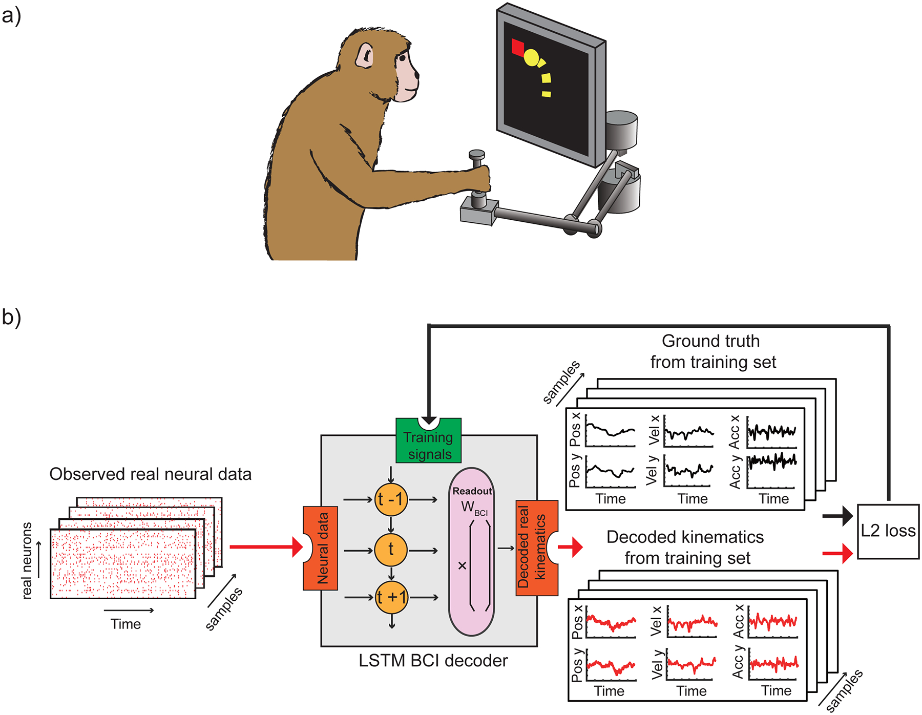
a, Experimental paradigm: monkeys were seated in front of a video screen and grasped the handle of a planar manipulandum that controlled the position of a cursor. Monkeys made reaching movements to a sequence of randomly-placed targets appearing on the screen while we recorded neural activity in primary motor cortex using an implanted electrode array. b, Training the baseline BCI LSTM decoder. Recorded spike trains are input to the BCI LSTM (Brain-Computer Interface, Long Short-Term Memory, a recurrent neural network that can learn to decode spike trains) decoder. The decoder outputs predicted kinematics, by first learning a time-varying generalizable internal representation (symbols t−1, t, t+1), and then mapping it to kinematic space (using readout weights WBCI). During training, actual kinematics (ground truth) are compared to the predicted ones using an L2 loss function (i.e., a Euclidean distance comparison) and used to refine the decoder (Methods).
Spike synthesizer and general structure.
Generative adversarial networks25–30 (GAN) can learn, end-to-end, a mapping from a random noise input to an output point that belongs to a desired data distribution. The process of training a GAN can be thought of as an adversarial game between a generator and a discriminator. The role of the generator is to produce fake data that seem real, while the discriminator learns to recognize whether data are real or fake. Competition in this adversarial game can improve both components until the generated fake data are indistinguishable from real data. The random noise input allows the GAN to synthesize different instances or variations around the desired target point. For example, in computer vision, after training a GAN on images of people with various hairstyles and clothes, the generator can synthesize, for any new person, many realistic-looking images of that person with different hairstyles26 or with different clothes27. Current deep generative models can only generate samples from the distribution they have been trained on. Thus, GANs cannot generalize to new kinds of data that they have never been trained with (for example, a GAN trained in images of shirts cannot generate images of pants).
Our synthesizer (Fig. 2, step 1, a sequential adaptation of a GAN) learns a direct mapping from hand kinematics to spike trains. This is achieved through the training of a new type of spike-based GAN (Methods, Extended Data Fig.1, step 1). After training, it can capture the embedded neural attributes. As with machine-vision GANs that cannot generalize from shirts to pants, here we expect that our model can synthesize new spike trains with good neural attributes for kinematics seen during training, but cannot generalize to new kinematics never encountered at training time. Next, new neural data from a second session, or a different subject, is split into training and test sets. The training set, which can be small (for example, 35 seconds of data), is used to adapt31,32 the synthesizer to the new domain (Fig. 2, step 2). Once adapted, the synthesizer outputs spike trains that emulate the properties of the new data, and thus can be used to assist the training of a BCI decoder for that session. To train the BCI decoder (Fig. 2, step 3), the synthesized spike trains are combined with the same limited training set that was used to adapt the synthesizer. We show that training on this combination of real and synthesized spike trains yields a better BCI decoder than training on the limited neural data alone, because the spike synthesizer notably increases the diversity and quantity of neural data available to train the BCI decoder. In essence, this achieves smart data augmentation33,34, whereby a limited amount of new real neural data combines with and adapts a previously learned mapping from kinematics to spike trains, delivering an updated mapping and synthesizer that can generate sufficiently realistic data to effectively train the BCI decoder.
Fig. 2 |. General Framework.
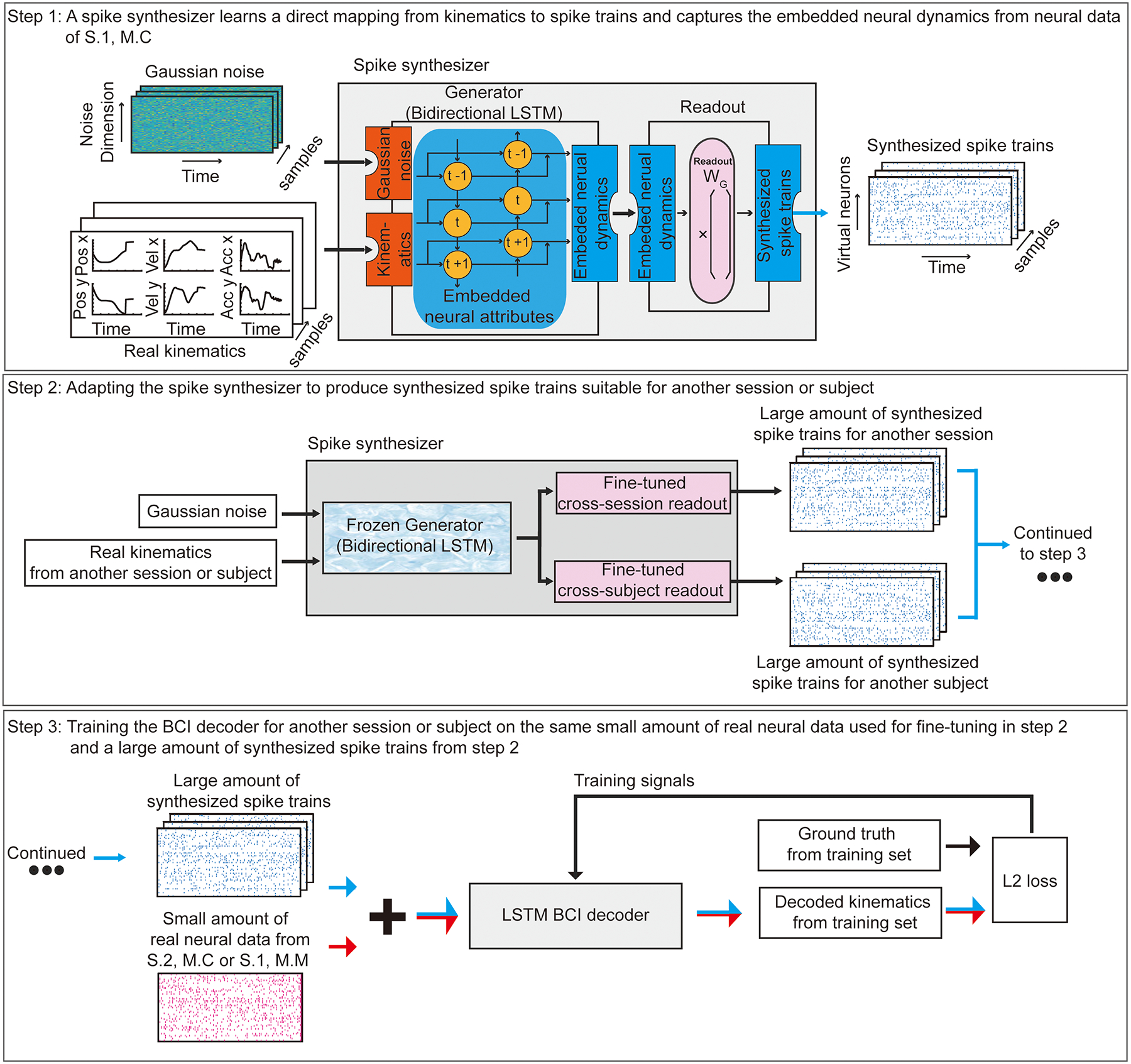
Step 1: Training a spike synthesizer on the neural data from session one of Monkey C (S.1, M.C) to learn a direct mapping from kinematics to spike trains and to capture the embedded neural attributes. Gaussian Noise and Real Kinematics are input to the Spike synthesizer (consisted of a Generator and a Readout). The spike synthesizer generates realistic synthesized spike trains by first learning the embedded neural attributes using a Generator (a bidirectional LSTM recurrent neural network) through a bidirectional time-varying generalizable internal representation (symbols t−1, t, t+1). Different instances of Gaussian Noise combined with new kinematics yield different embedded neural attributes that all have similar properties to those used for training. Then, the Readout maps the embedded neural attributes to spike trains (using readout weight WG). Step 2: Adapting the spike synthesizer to produce synthesized spike trains suitable for another session or subject from Real Kinematics and Gaussian noise. We first freeze the generator to preserve the embedded neural attributes or virtual neurons learned previously. Then, we substitute and fine-tune the readout modules using a limited neural data from another session or subject (session two of Monkey C (S.2, M.C) or session one of Monkey M (S.1, M.M)). The fine-tuned readout modules adapt the captured expression of these neural attributes into spike trains suitable for another session or subject. Step 3: Training a BCI decoder for another session or subject using the combination of same small amount of real neural data used for fine-tuning (in step 2) and a large amount of synthesized spike trains (in step 2).
Validation of the spike synthesizer using a random reaching task.
We trained the spike synthesizer on session one of Monkey C, and characterized both the recorded and virtual neurons using properties such as firing rates and position, velocity and acceleration activity maps. In addition, we measured the correlations between the recorded real and virtual neurons.
Can the spike synthesizer synthesize spikes with realistic position (velocity, acceleration)-related activity? To answer this question, we compared the position, velocity and acceleration activity maps built from synthesized spikes trains to those of actual spikes. We counted the number of spikes for different hand positions and normalized them with respect to the averaged spike counts across the workspace. Fig. 3a,i shows the normalized position activity map for real neuron 35, and Fig. 3a,ii shows its virtual counterpart. The mean square error (MSE) between the two maps is 0.0086, which in this example is lower than the trimmed average MSE between real neurons (0.13, based on 99% samples). The position activity maps have similar light and dark spots. Fig. 3a,iii shows the normalized position activity map for real neuron 3, and Fig. 3a, iv shows its virtual counterpart. The MSE between the two maps is 0.21, higher than the average MSE. In this example, the position activity maps exhibit similar overall features but differ slightly in the exact location of the peaks. Fig. 3b shows a summary position histogram for all real–virtual neuron pairs. The histogram is left-skewed, around the mean of 0.13. Sixty-one of sixty-nine neurons (88%) had an error less than the trimmed average. Supplementary Fig. 5 (Supplementary Fig. 6) shows a summary velocity (acceleration) histogram for all real–virtual neuron pairs. Those histograms are left-skewed, with a trimmed mean of 0.11 (0.10). Sixty of sixty-nine neurons (87%) had an error less than the average. This shows that, with respect to position (velocity, acceleration)-related activity, the model has learned realistic virtual neurons.
Fig. 3 |. Normalized position activity map, constructed as the histogram of neural activity as a function of position.
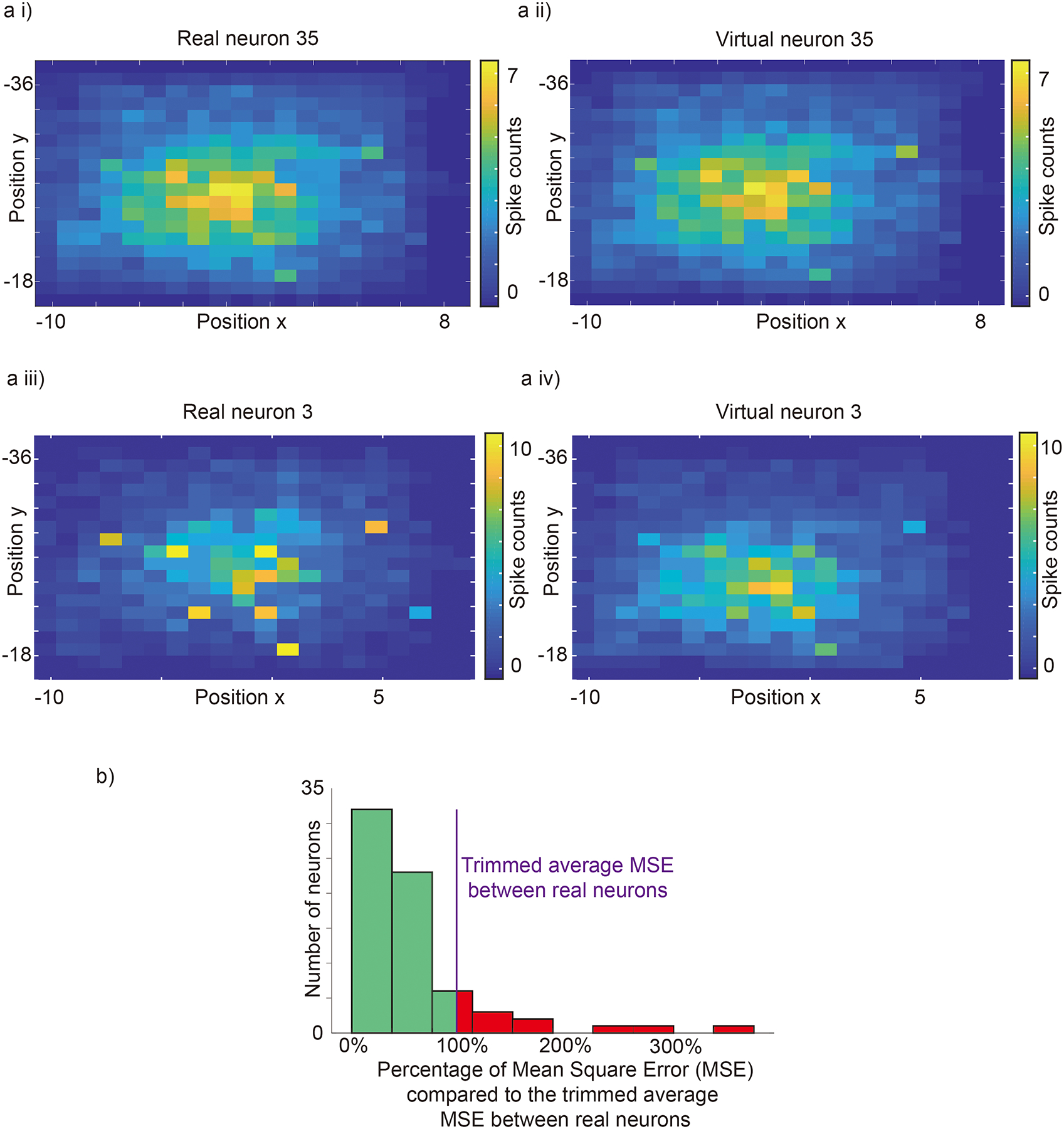
a i,Position activity map for real neuron 35 normalized across the workspace. a ii, corresponding position activity map for virtual neuron 35. a iii, a iv, Position activity maps for real and virtual neuron 3. b, Histogram of mean squared error between the real and generated activity maps for all neurons. The purple line is the trimmed averaged mean square error (based on 99% samples, 0.13) between real neurons. It provides a reasonable bound for quantifying the difference between real and virtual neurons.
Can the spike synthesizer synthesize spikes with realistic firing patterns? We then asked whether the spike synthesizer can learn to synthesize spike trains from specific kinematics (Fig. 4a), with realistic firing rates (Fig. 4b,c). We found that the spike synthesizer produces firing rates (distribution of firing rates across all neurons) that are not different from the those of real neurons (Fig. 4.d; Kolmogorov–Smirnov test: the samples are not from different distributions with p=0.1536).
Fig. 4 |. synthesized spike trains generated from specific kinematics.
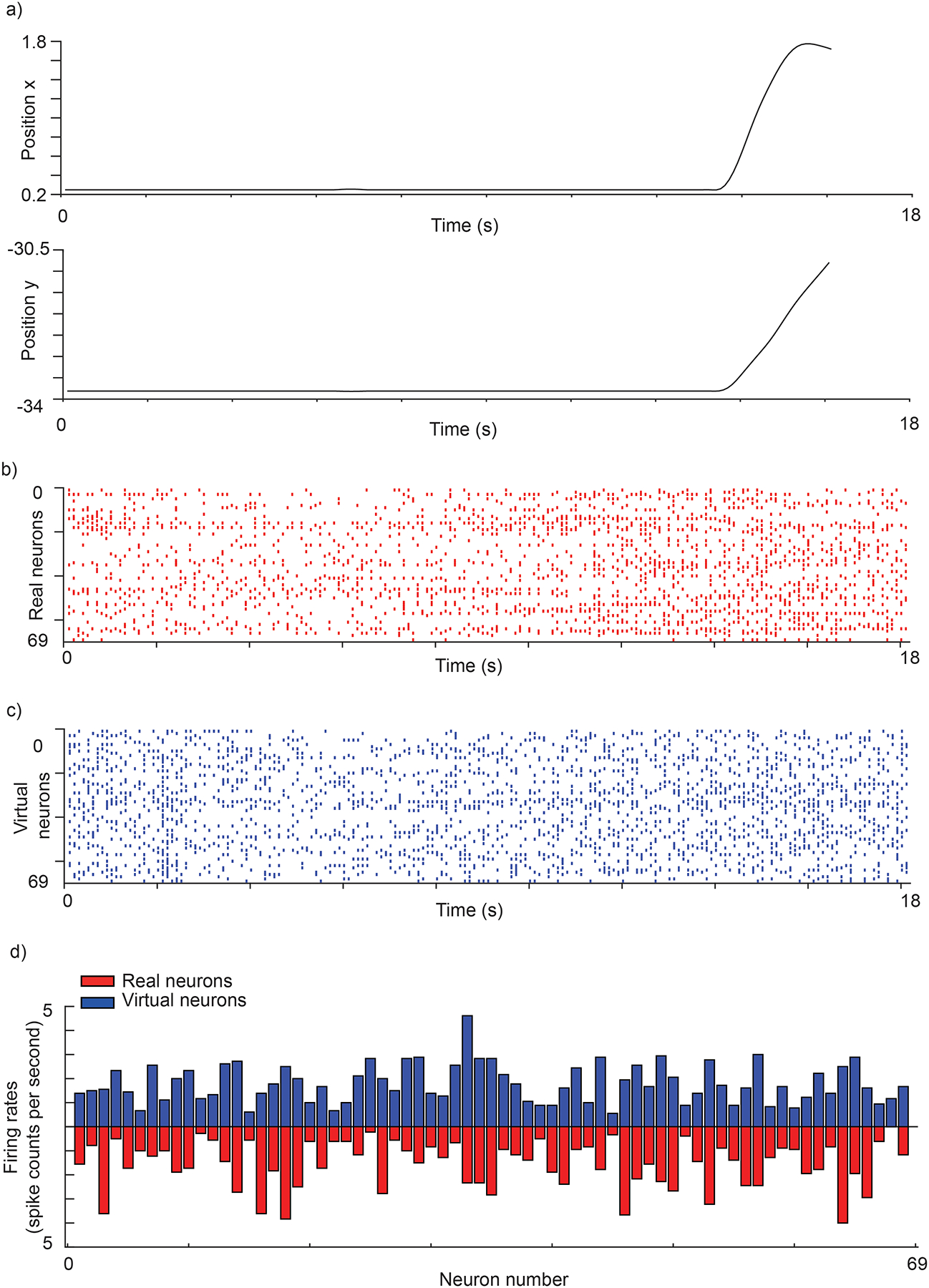
a, Movement kinematics (position). b, Real neural data for the kinematics in (a). c, Synthesized spike trains from the spike synthesizer for the kinematics in (a). d, firing rates (distribution of firing rates across all neurons) for the kinematics in (a) for real and virtual neurons.
Then, we asked whether the synthesized spike trains are correlated with real spike trains more than would be expected by chance. To assess this, we used pairwise correlations computed after placing the spikes in 250-ms time bins35, a time scale relevant to behavioral movements. We compared the correlation coefficients between pairs of real and synthesized spike trains to those between real spike trains and those generated by a homogenous Poisson process, an estimate of chance level (see Methods for an alternate measure that uses randomly shuffled real spike trains). The correlation coefficient is equal to one if spike trains are identical, and zero if they are independent. Fig. 5a,i shows a time series of binned spike counts for neuron 8 (an example from the left portions of Supplementary Fig. 3b), with a correlation between synthesized and real neural data of 0.59. In comparison, the correlation (Fig. 5a,ii) between the neural data from a homogeneous Poisson distribution and real neural data is 0.03. Fig. 5a,iii shows similar plots for neuron 59 (an example from the right portions of Supplementary Fig. 3b). Here, the correlation between actual and synthesized data is 0.18, whereas that between real neural and homogeneous Poisson data is 0.07 (Fig. 5a,iv). In summary, for 91% (63 out of 69) of the neurons (Fig. 5b), the correlations of the actual spike trains with synthesized trains were higher than the correlations between neural spikes of randomly shuffled neurons.
Fig. 5 |. Correlation between synthesized and real spike trains.
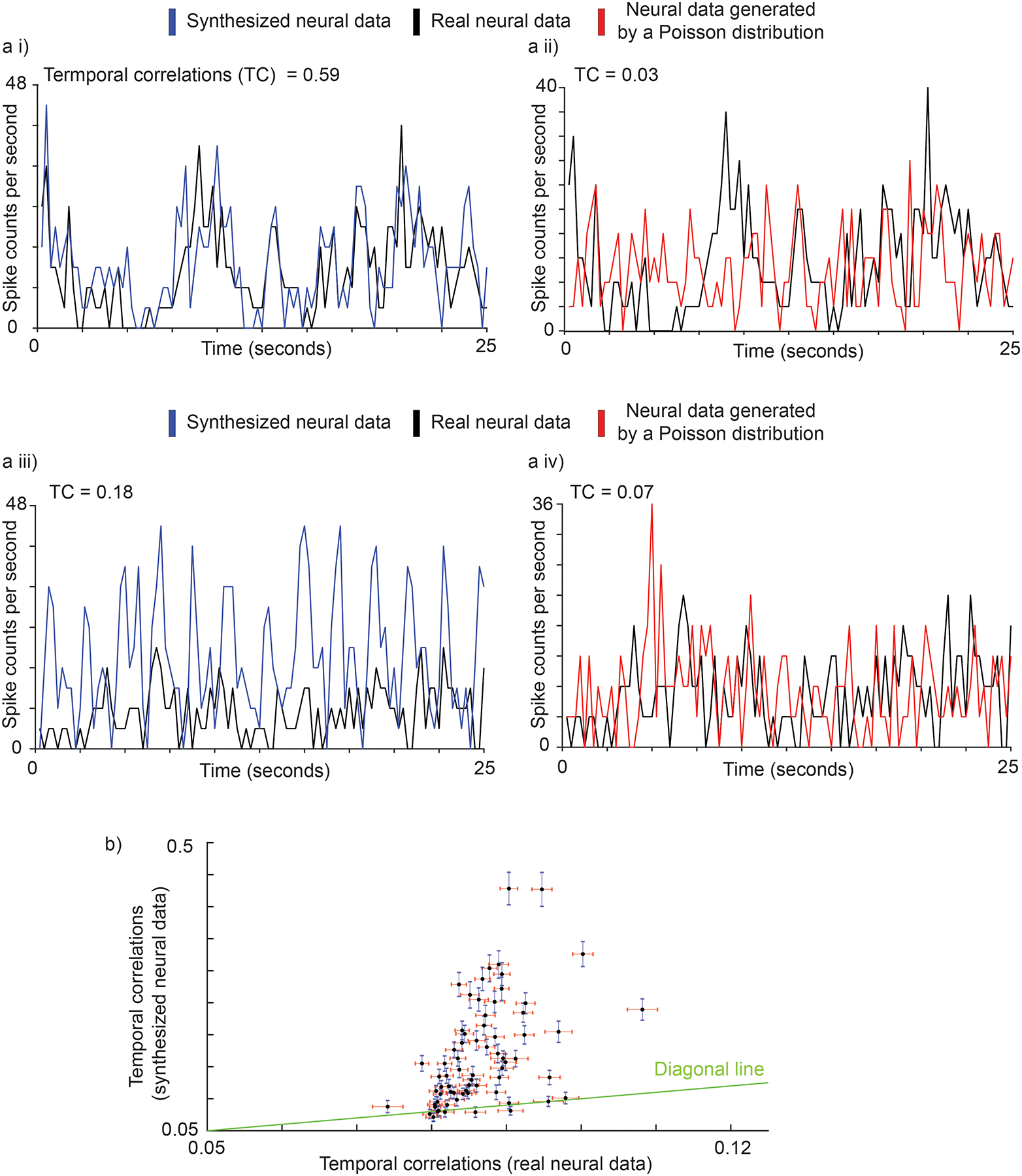
a i, a ii, Time series of binned spike counts for neuron 8 (good example, left portions of Supplementary Fig. 6.b). Correlation between synthesized and real neural data is 0.59. In contrast, correlation between generated (red, from a Homogeneous Poisson distribution) and real (black) neural data is 0.03. a iii, a iv, Time series of binned spike counts for neuron 59 (bad example, right portion of Supplementary Fig. 6.b). Correlation between synthesized neural data and real neural data is 0.18, while correlation between generated neural data from Poisson distribution and real neural data is 0.07. b, Scatter plot for synthesized neural data vs. randomly shuffled real spike trains baseline. Each black point represents a neuron. The vertical axis is the correlation between synthesized and real neural data across all neural spike train samples for each neuron with blue standard error bar (mean + / − S.E., sample number = 63). The horizontal axis is the correlation between neural data of randomly shuffled neurons across all neural spike train samples with red standard error bar (mean + / − S.E., sample number = 63).
In summary, the spike synthesizer learned to generate spike trains that are better correlated with real spike trains than one would expect by chance, although some differences are apparent between real and synthesized data. Therefore, we then assessed whether the synthesized spike trains are sufficiently realistic to effectively assist the training of a BCI decoder, which is the primary goal of this study.
Synthesized neural spikes can accelerate the training and improve the generalization of cross-session and cross-subject decoding.
To test the utility of our spike synthesizer, we explored whether it can accelerate the training and improve the generalization of a BCI decoder across sessions and subjects. We trained the spike synthesizer from the data of the first session of Monkey C (S.1, M.C, Fig. 2. step 1). Then, we split new neural data from a second session, either from the same subject (session 2 of Monkey C; S.2, M.C) or from a different subject (first session of Monkey M; S.1, M.M), into training and test sets. We froze the generator of the spike synthesizer to preserve the embedded neural attributes. Then, we fine-tuned the readout module of the spike synthesizer with as little as 35 seconds of the new training set to learn its dynamics. After training the BCI decoder with various combinations of real and synthesized data, we tested it on an independent test set from another session (S.2, M.C) or subject (S.1, M.M), and compared the decoding performance to other data augmentation methods (Supplementary Information). These included either using real neural data alone (real-only) to train the BCI decoder, or three other data augmentation methods: real augmentation (duplicate and concatenate available real neural data), stretch augmentation (duplicate, randomly stretch, and concatenate available real neural data) and mutation augmentation (duplicate, add noise, and concatenate available real neural data).
The spike synthesizer can synthesize spikes with realistic position (velocity, acceleration)-related activity.
We first tested whether synthesized spike trains can accelerate training for cross-session decoding. When using less than 17 minutes of new data from S.2, M.C to train the BCI decoder, our GAN augmentation method performed better than the other augmentation methods (Extended Data Fig. 2), and the real-only method (Fig. 6.a). Without any data augmentation, the BCI decoder needed at least 8.5 minutes of training data to converge. However, using our spike synthesizer it becomes possible to train the BCI decoder with substantially fewer real data. At the extreme, with only 35 seconds of new neural data (S.2, M.C), augmented by 22 minutes of synthesized data, cross-session decoding performance was better than for competing methods (used to extend the original 35 seconds of new data to 22 minutes). The averaged best performance for all kinematics (the lowest point for each curve in Fig. 6.b) of the GAN-augmentation method was 7.2%, 4.8%, 5.6% and 16% better than the stretch-augmentation, mutation-augmentation, real-concatenation, and real-only methods, respectively. Fig. 6c shows general performance results for all kinematics variables over the percentage of new neural data used, demonstrated with a format similar to receiver operating characteristic (ROC) curves. The area under the GAN-augmentation curve was 0.030, 0.020, 0.015, and 0.33 greater than for the stretch-augmentation, mutation-augmentation, real-concatenation, and real-only methods, respectively. To achieve accuracy saturation (Fig.6.d, >=95% of the peak for the real-only method of training on all neural data from S.2, M.C), GAN-augmentation only requires 1.82 minutes additional neural data from S.2, M.C, compared to 5.47, 6.02, 8.67 and 12.93 minutes (4.27x, 4.70x, 6.77x and 10.10x) for mutation-augmentation, real-concatenation, stretch-augmentation and real-only, respectively. The real-only method requires 8.8 minutes of additional neural data to converge, and achieves 0.77 for average correlation coefficient across kinematics. In comparison, GAN-augmentation requires only 0.67 minutes of additional neural data to achieve the same performance. In summary, our GAN-augmentation is the best among all tested methods for cross-session BCI training.
Fig. 6 |. Cross-session decoding.
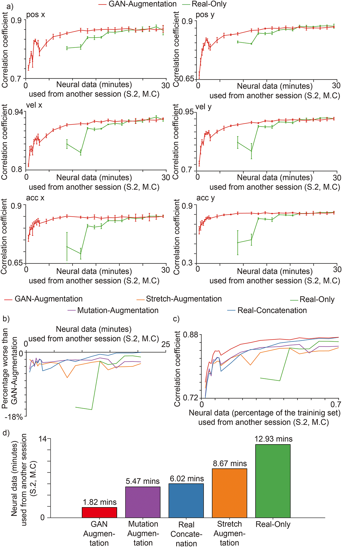
There are six methods: GAN-augmentation (red) mutation-augmentation (purple), stretch-augmentation (orange), real-augmentation (blue), real-only (green). The cut-off time for (b) and (c) is 20.53 minutes - the minimum amount of time needed for other methods to achieve performance comparable to GAN-augmentation. a, The performances for each kinematic in 5-fold cross-validation. The horizontal axis is the number of minutes of neural data from the session two of Monkey C used. The vertical axis is the correlation coefficient (mean + / − S.D., n = 5 folds) between the decoded kinematics and real kinematics on an independent test set from the session two of Monkey C. Synthesized spike trains that capture the neural attributes accelerate the training of a BCI decoder for the cross-session decoding. b, Average percentage performances worse than GAN-augmentation method. The horizontal axis is the number of minutes of neural data from the session two of Monkey C used. The vertical axis is the average performance for all six kinematic signals of each method worse than the average percentage performance of GAN-augmentation method. c, Average performances presented similar to receiver operating characteristic (ROC) curve. The horizontal axis is the percentage of neural data from the training set of session two of Monkey C used. The vertical axis is the same as a). d, Amount of additional neural data (S.2, M.C) needed for each method to achieve accuracy saturation (>=95% of the peak for real-only method training on all neural data from S.2, M.C).
Synthesized spike trains can also accelerate the training for cross-subject decoding. When using less than 9 minutes of new data from S.1, M.M to train the BCI decoder, our GAN augmentation method performed better than the other augmentation methods (Extended Data Fig. 3), and the Real-Only method (Fig. 7.a). Without any data augmentation, the BCI decoder needed at least 8.5 minutes of training data to converge. Fig. 7.b shows the general performance results for all kinematics variables over a wide range of new neural data. The averaged best performance for all kinematics (the lowest point for each curve in Fig. 7.b) of the GAN-augmentation method is 60%, 17%, 11% and 6% better than the stretch-augmentation, mutation-augmentation, real-concatenation and real-only methods. Fig. 7.c shows general performance results for all kinematics variables over the percentage of new neural data used, demonstrated with a similar format as ROC curves. The area under the GAN-augmentation curve was 0.11, 0.052, 0.039, and 0.58 greater than the stretch-augmentation, mutation-augmentation, real-concatenation, and real-only methods, respectively. None of the tested methods achieved performance comparable to GAN-augmentation, since the GAN-augmentation method can transfer learned dynamics and improve the decoding performance beyond the best performance achievable on data from Monkey M alone. (Further explained in the following section). To achieve accuracy saturation, GAN-augmentation only needs 0.1 minutes of additional neural data from S.1, M.M, compared to 1.25, 2.65, 4.02 and 8.67 minutes (12.50x, 26.50x, 40.20x and 86.70x) for real-concatenation, mutation-augmentation, stretch-augmentation and real-only, respectively. Thus, our GAN-augmentation is again the best among all tested methods for accelerating cross-subject BCI training.
Fig. 7 |. Cross-subject decoding.
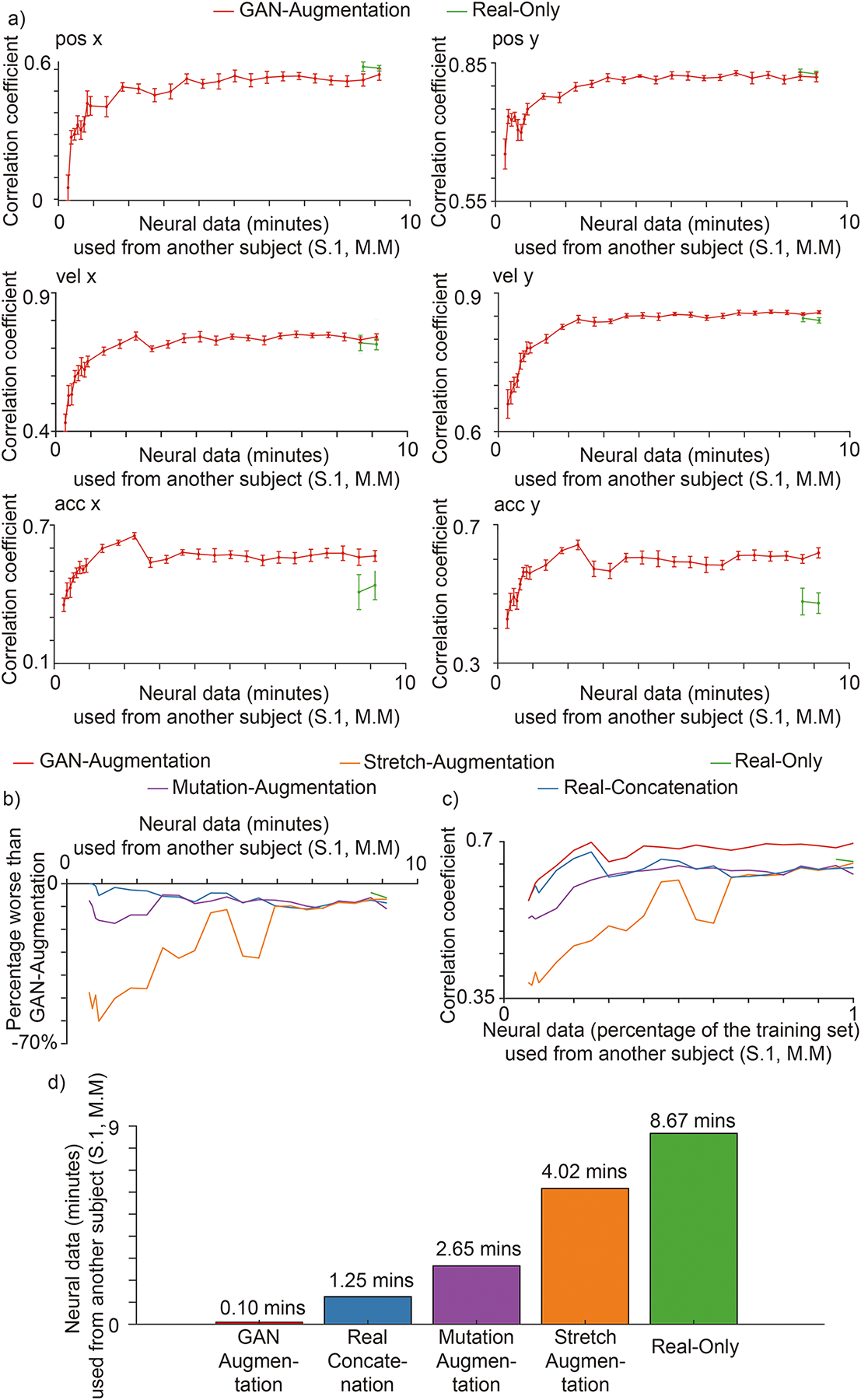
Methods and their notations are the same as that of Fig. 6. a, Performances for each kinematic in 5 folds cross-validation. The horizontal axis is the number of minutes of neural data from Monkey M used. The vertical axis is the correlation coefficient (mean + / − S.D., n = 5 folds) between the decoded kinematics and real kinematics on an independent test set from the Monkey M. When the neural data from another subject is limited, synthesized spike trains that capture the neural attributes accelerate the cross-subject decoding performance. In addition, synthesized spike trains have learned generalizable information that can boost cross-subject decoding performance on acceleration over the best achievable performance. b, Average percentage performances worse than GAN-augmentation method. The horizontal axis is the number of minutes of neural data from the session one of Monkey M used. The vertical axis is the same as Fig. 6. b. c, Average performances presented similar to receiver operating characteristic (ROC) curve. The horizontal axis is the percentage of neural data from the training set of session one of Monkey M used. The vertical axis is the same as (a). d, Amount of additional neural data (S.1, M.M) needed for each method to achieve accuracy saturation (>=95% of the peak for real-only method training on all neural data from S.1, M.M).
Transferring learned dynamics and improving beyond the best-achievable cross-subjects decoding.
Training a spike synthesizer that learns good neural attributes from Monkey C (with its better decoding performance) might transfer useful information to boost cross-subject decoding performance beyond the best achievable on data from Monkey M alone. When neural data are ample for both Monkey C (Fig. 5.a i) and Monkey M (Fig. 6.a), the decoding performance on position and velocity are equally good for both monkeys, though the performance on acceleration of Monkey C is better than that of Monkey M (0.85 vs. 0.43 for acc x; 0.82 vs. 0.48 for acc y). The better decoding performance on acceleration data from Monkey C might come from the better quality of signals collected by the electrode arrays, or from the fact that neural data from Monkey C is inherently easier for the decoder than that from Monkey M. A lower quality of the collected neural data from Monkey M might decrease the decoding accuracy of accelerations, because accelerations are the usually hardest to decode; but this could be improved through prior learning from monkey C. Since decoding performance on position and velocity for monkey M are already good, we wondered whether any useful information learned from neural data of Monkey C could improve the best achievable decoding performance on acceleration for Monkey M.
Here, we compared the best achievable performance of all methods (the highest points for acceleration x and acceleration y curves in Fig. 7.a and Extended Data Fig. 3). As a result, for acceleration y, the best achievable performance for GAN-augmentation was 0.64, significantly better than the best achievable performance for Real-Only (0.48; p = 10−14, t-test), stretch-augmentation (0.62; p = 10−3, t-test), mutation-augmentation (0.51; p = 10−11, t-test) and real-concatenation (0.59; p = 10−4, t-test). The results for acceleration x are similar as that of acceleration y. Thus, even with ample neural data for both monkeys, the neural attributes learned from the first monkey can transfer some useful information to improve the best achievable decoding performance for the second monkey.
Discussion
The intuition of this paper is that building a spike synthesizer that captures underlying neural attributes can accelerate the training and improve the generalization of BCI decoders. We have introduced a new spike synthesizer that can learn a mapping from kinematics to neural data. The spike synthesizer captures and reproduces the neural attributes in its training set. After the fine-tuning procedure, we showed that the synthesizer adapted to data from a new session or even a new subject, and can synthesize new spike trains. The synthesized spike trains can accelerate the training of a BCI decoder and improve its generalization across sessions and subjects.
We could interpret the improvement in the decoding performance from the perspective of statistics of movements. The understanding of the statistics of movements can help us in many situations where obtaining simultaneous recordings of both neural activity and kinematics is difficult. It has been shown36 that distribution-alignment decoding (DAD) can leverage the statistics of movements to achieve semi-supervised decoder training. The authors built prior distributions of motor-output variables during a simple planar reaching task. DAD was then able to align the distributions of decoder outputs to kinematic distribution priors. However, it is not clear whether the approach would work in more complex movements, as one would need many prior distributions of motor-output variables (high-level templates). The complex movements might involve sub-movements such as holding still, rapid reaching and slow reaching. It might take a substantial amount of time to craft these templates manually, and it is hard to choose the right form of the templates for a task and to combine them properly. In comparison, our spike synthesizer recreated neural attributes such as position, velocity and acceleration activity maps, velocity neural tuning curves (low-level templates) directly from the data. For more complex kinematics, our spike synthesizer might synthesize spike trains drawn from different distributions for holding and rapid reaching by combining those neural attributes in an autonomous way. There is no need to handcraft high-level templates (prior distributions of motor-output variables) if they can be constructed from more fundamental low-level ones.
The neural attributes captured by the spike synthesizer (position, velocity, acceleration activity maps and velocity neural tuning curves, Supplementary Figs. 1,2,5,6) have a special name in the literature37–42: motor primitives. Motor primitives are a generalization of movement components or the templates (kinematic distribution priors) used by DAD. It has been suggested that the motor cortex may control movement through flexible combinations of motor primitives, elementary building blocks that can be combined to give rise to complex motor behavior. One study41 defined a motor primitive as the directional neural tuning curve for each neuron, fitted by a Gaussian function. The authors built movement trajectories through linear combinations of those tuning curves. Related research42 used gain patterns over neurons to predict movement trajectories. Another study described43 the learning of a diverse set of motor primitives through a latent representation of a neural abstraction network from kinematics given in demonstration. Then, the authors split new complex kinematics into subparts, and fit those subparts with the motor primitives. The key problem in motor-primitive research is how to learn the primitives, and then how to combine them to create complex motion. Here, our results suggest that our spike synthesizer learned motor primitives through its internal representation (similar to the work in ref.43) from both kinematics and neural data (in contrast to the work in ref.43, where only kinematics was used) and their combination rules in an autonomous and principled way. In addition, from an extended version41 of the definition of a motor primitive that includes both position and velocity tuning for each neuron, we can reproduce these motor primitives by reconstructing position and velocity tuning curves for each neuron from the internal representation.
A recent method20 can infer latent dynamics from single-trial neural spike data by leveraging a deep learning auto-encoder (LFADS). Our method is complementary to this work in the following ways. First, LFADS focuses on how to construct a mapping from the neural data to low-dimensional latent variables (neural population dynamics), while simultaneously reconstructing the same neural data from a Poisson process parameterized by these low-dimensional latent variables. In contrast, our method uses a generative adversarial network to create a mapping directly from the kinematics to the neural data in an end-to-end manner. In addition, the mapping does not impose any prior distribution on the data.
Recent advances in the analysis of neural population activity, especially with the help of BCI methods, have revealed the importance of the covariance structure of neuronal populations in controlling movements and motor skill acquisition44–46. Although, in our work, the spike synthesizer was trained to learn a mapping between kinematic and neural data, internally, the spike synthesizer maps the kinematics to a generalizable internal representation that captures embedded neural attributes, including the high-order statistics between neurons such as covariance. We expect this covariance structure imposed by our generalizable internal representation between neurons can accelerate training for BCI decoders that even aim to generalize across tasks. Finally, our framework of learning the internal representation from raw data and additional synthesized data is general and fully data-driven, in contrast to neural encoding models47–50 that assume Gaussian or Poisson distributions. Hence, our framework could be applied to other neuroscience encoding and decoding problems beyond motor control with minimal too domain-specific modifications.
Methods
The BCI decoder.
We use the state-of-the-art Long Short-Term Memory (LSTM) network10,11 as the decoder. Recurrent neural networks can use their feedback connections to store a representation of recent input in the hidden states. However, with the traditional backpropagation through time to update the hidden states, they often suffer either a gradient exploding or vanishing problem. Long Short-Term Memory creates an uninterrupted gradient flow and thus have a better performance. The structure of LSTM cell can be formalized as
| (1) |
| (2) |
| (3) |
Where xt is the input at time t and ht is the hidden dimension at time t. W is the weight vector from ht−1 and xt to gates. σ is the sigmoid function. i is the input gate, deciding whether to write to cell. f is the forget gate, deciding whether to erase the cell. g is the gate gate, deciding how much to write to the cell. o is the output gate, deciding how much to reveal cell. ct is the middle variable. In the LSTM decoder case, we unroll our LSTM cell and consider 200 timesteps for each sample. The input dimension is (N, T, D), where N is the number of samples, T is the number of timesteps, D is the feature dimensions. Our input is batched neural spikes where there are 128 samples, 200 timesteps and number of neurons (69 for session 1, 77 for session 2 of Monkey C, 60 for session 1 of Monkey M) for feature dimensions. The hidden dimensions h is 200 for the LSTM decoder. So, we have an output dimension (N 128, T 200, H 200) from LSTM decoder. We feed this output into a fully connected layer to produce the kinematics (dimension [128, 200, 6]). We apply dropout techniques47 and learning rate decay48 while training the LSTM decoder.
Bidirectional LSTM49.
The output of a sequence at a current time slot relies not only on the sequences before it, but also depends on the sequences after it. So, to better capture the neural attributes, we use the bidirectional LSTM to build the generator and discriminator in our Constrained Conditional LSTM GAN model. At each time-step t, this network has two hidden states, one for left-to-right propagation and another for the right-to-left propagation. The update rule is
| (4) |
| (5) |
Where and maintain the left-to-right hidden state and right-to-left hidden state separately at time t. g is the LSTM cell update function in Equation (1), (2), (3).
Generative adversarial network (GAN).
GANs21 provide a tool to learn a map from a random noise input to the desired data distribution in an end to end way, updating its parameters via backpropagation50. Thus, it does not require any assumption about the data distribution. It is purely data-driven and does not need a strong prior model which would limit the generality. The process of training a GAN can be thought as an adversarial game between a generator and a discriminator. The role of the generator can be thought of as to produce fake currency and use it without detection, while the discriminator learns to detect the counterfeit currency. Competition in this adversarial game can improve both components’ abilities until the counterfeits are indistinguishable from real currency. After this competition, the generator can take random noise (that provides variations) as input to output different kinds of realistic bills with different textures. Several approaches have been proposed for image synthesis using GANs, enhanced to be able to generate output images for a particular object class, such as conditional GAN25, Semi-Supervised GAN27, InfoGAN28, AC-GAN26 and cGANs29. In this fake currency scenario, by injecting the conditions (Denomination of each bill) into the input of GAN, we can select which kind of bills we want to generate (e.g., a 100-dollar bill), while the noise provides the varied texture of the bills (e.g., smooth or wrinkled).
Constrained Conditional LSTM GAN (cc-LSTM-GAN, the spike synthesizer):
We propose the constrained conditional LSTM GAN to model the behavior of M1 from the kinematics. A normal LSTM model takes input which has a dimension of (N, T, D) where N is the number of samples in one minibatch, T is the time horizon, D is the hidden dimension size. We chose 2 seconds as time horizon in our experiments. the first input dimension, N is the number of batches. The third input dimension, D, is the number of neurons for the discriminator or noise dimension for the generator. For each item in the batch, we have a 2 second slice of neural spikes from D neurons. Since the number of neurons is the third hidden dimension of the LSTM in the discriminator, our discriminator treats different neurons as individuals that have different neural tuning properties. Thus, the CC-LSTM GAN encoding model is a multiple neural encoding model.
Training assistant LSTM decoder (GAN-ta LSTM decoder).
We train a LSTM decoder (hidden dimension h: 200) on neural data ([N,T,M], where N is the sample size 128, T is the time horizon 200, M is the number of neurons (69 for S.1, M.C, 77 for S.2, M.C, 60 for S.1, M.M)) from one monkey and freeze its parameters when we train our Constrained Conditional Bidirectional LSTM GAN. This decoder applies constraints to the cc-LSTM-GAN. We want to maintain the decoding performance while we train the spike synthesizer.
Bidirectional LSTM generator.
The bidirectional-LSTM generator takes Gaussian noise ([N, T, D], where N is sample size 128, T is time horizon 200, D: Dimension for Gaussian noise 6) and real kinematics ([N, T, D] where N is sample size 128, T is time horizon 200, D: Dimension for kinematics 6) as inputs and synthesizes the corresponding spikes trains. We feed the outputs (dimensions [N, T, 2*H], where N is the Sample size 128, T is the time horizon 200, H is the hidden dimension 200) of the bidirectional-LSTM into a fully connected layer to synthesize spikes trains with the correct number of neurons (dimensions [N,T,M] where N is the sample size 128, T is the time horizon 200, M number of neurons (69 for S.1, M.C, 77 for S.2, M.C, 60 for S.1, M.M)). We apply function51 as the output layer of the fully connected layer which maps a real value to [−0.5, 0.5] that gives us a probability representation of whether the current bin contains a spike event or not. For example, if the value in the current bin is −0.3, the probability there is a spike event in this bin is 0.2 (−0.3 + 0.5). Here, for analysis, we sample Bernoulli distribution to generate the neural firing patterns. While, for decoding, the LSTM decoder directly takes the probability as an input.
Bidirectional LSTM discriminator.
The Discriminator is a bidirectional-LSTM. It takes the synthesized spikes trains ([N,T,M], where N is the sample size 128, T is the time horizon 200, M is the number of neurons (69 for S.1, M.C, 77 for S.2, M.C, 60 for S.1, M.M)) and neural data ([N,T,M], N,T, M have the same meaning and dimension as synthesized spike trains) as inputs and learns to determine whether a sample is from the neuron data or synthesized spikes trains. We feed the outputs (processed by a sigmoid activation) of the bidirectional-LSTM into a fully connected layer to obtain a decision value (0,1), a probability that decides whether the current sample is real or fake. We feed the output of a bidirectional-LSTM into another fully connected layer to get the decoded kinematics. This helps us to apply the category constraints.
Multiple neural encoding model (CC-LSTM-GAN).
we use a conditional structure that has a GAN category loss to let the discriminator distinguish both data source distribution (neural spikes) and data label distribution (kinematics corresponding to these spikes). When the input of the bidirectional LSTM discriminator is the neural data (synthesized spikes trains), the real (fake) embedding features are the output of bidirectional LSTM discriminator. GAN embedding category loss is the L2 loss between the real embedding features and the fake embedding features.
| (6) |
When the input of bidirectional LSTM discriminator is the neural data (synthesized spikes trains), the real (fake) decoded kinematics are the output of the fully connected layer after the bidirectional LSTM discriminator. Real (fake) GAN decoding category loss is the L2 loss between real (fake) decoded kinematics and real kinematics. The GAN category loss is the average of real GAN decoding category loss, fake GAN decoding category loss and GAN embedding category loss.
| (7) |
To maintain the source distribution, our cc-LSTM-GAN needs to play the min max game. We need to minimize discriminator GAN loss (LD) and generator GAN loss (LG). The LD and LG
| (8) |
| (9) |
Where z is the Gaussian noise, x is the neuron spikes, k is the kinematics, p(z) is the noise distribution, pdata is the data distribution. LD is the discriminator loss calculated by cross entropy loss function, LG is the generator loss calculated by cross entropy loss function.
To further maintain the statistical structure of the real neurons, we want to maximize the inner product loss between the neural data and synthesized spikes trains. Thus, we have our inner product loss
| (10) |
The pre-trained GAN-ta LSTM decoder takes the neural data and synthesized spike trains as input and decodes the corresponding kinematics. The decoded generated kinematics are kinematics decoded from synthesized spike trains. The decoded real kinematics are kinematics decoded from neural data. We apply L2 loss between real kinematics and decoded generated kinematics. We apply L2 loss between decoded generated kinematics and decoded real kinematics. The pre-trained GAN-ta LSTM decoder helps our generator synthesize more realistic spike trains in terms of the performance of GAN-ta LSTM decoder.
The total generator loss is the weighted average of the generator GAN loss (LG), the GAN category loss, the inner product loss, the L2 loss between decoded generated kinematics and decoded real kinematic and the L2 loss between decoded generated kinematics and real kinematics.
| (11) |
The total discriminator loss is the weighted average of the discriminator GAN loss (LD) and the GAN category loss. We train this network by real GAN training set (a subset of the neural data from the first monkey) and minimize the total discriminator and generator losses.
| (12) |
Fine tuning
We trained CC-LSTM-GAN on the session one data of Monkey C. In the finetuning process, we took a limited amount of neural data from session one of Monkey C (cross-session) or a from Monkey M (cross-subject). We added another fully connected layer (Readout module) on top of the bidirectional LSTM generator and used it to generate the corresponding neural spikes with the same number of neurons as the added data. We froze the parameters of hidden units from the bidirectional LSTM generator and only trained this new fully connected layer with limited new data. The loss function of the finetuning process is the inner product loss in Equation (10). Then, we fed the kinematics corresponding this limited amount of neural data into the Generator multiple times to synthesize a large amount of spike trains.
Correlation
To calculate the correlations across neural spike train samples for each neuron, we parsed the synthesized and real neural spike into 250ms bins and set the time horizon to 25s. We calculated the correlations for each sample and averaged the absolute value of correlations for each neuron. We compared the result against that of randomly shuffled real spike trains (compared the real neural data with shuffled neural data from other neurons) and that of the neural spikes generated from a homogeneous Poisson distribution. For homogeneous Poisson distribution, it assumes that the generation of each spike depends only on a homogeneous firing rate and is independent of all the other spikes. Thus, it is a good baseline for comparison.
Data Augmentation
We used multiple data augmentation methods to train a BCI decoder and achieve a better decoding performance than training a BCI decoder on the neural data only. The start point of limited neural data is always selected from the start of the neural data in each fold. The end point of the limited neural data is the start point plus the length of the required amount of limited data.
Real-only method:
Without any data augmentation, we trained the BCI decoder on the neural data only and tested on the neural data of an independent test set. This method required at least 8.5 mins neural data in the training set to let the BCI decoder converge (The criteria of convergence are that the training loss would decrease slowly during training. If we have less than 8.5 minutes of training data, the training loss does not decrease no matter for how long we train the LSTM BCI decoder). If the BCI decoder fails to converge, the correlation coefficient is defined as correlation between randomly shuffled real kinematics and real kinematics (0.00027, chance level)
Real-concatenation:
We took a limited amount of neural data from the training set and concatenated it multiple times until it has the equal or longer length than the whole training set. We trained the BCI decoder on the concatenated neural data and tested on the neural data of an independent test set.
Mutation-augmentation:
We flipped the value of the limited neural data with 5% probability (spike to non-spike or non-spike to spike). We repeated this step several times and concatenated the mutated neural data and its kinematics until they had equal or longer length than the whole training set. We trained the BCI decoder on the mutated neural data and tested on the neural data of an independent test set.
Stretch-augmentation:
We stretched the limited neural data by 10 percent and filled the empty stretched slots of the neural data by zero or one (50% probability). We calculated the averaged absolute gradients for each kinematic signal for each slot. We filled the empty stretched slots of the kinematics by adding or subtracting (50% probability) the value of the last slot with the averaged absolute gradients. We repeated the above steps several times and concatenated the stretched neural data and its kinematics together until it had equal or longer length than the whole training set. We trained the BCI decoder on the stretched neural data and tested on the neural data of an independent test set.
GAN-augmentation:
We combined the synthesized spike trains (22 minutes in our paper) with the augmented data from Real-Concatenation method. We trained the BCI decoder on the combination of synthesized spike trains and concatenated neural data and tested on neural data of an independent test set.
Extended Data
ED Fig. 1. General Framework.
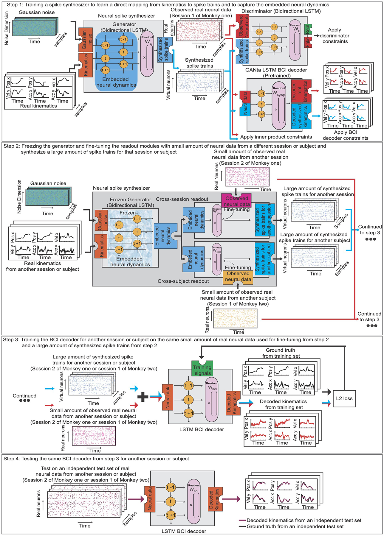
Step 1: training a neural spike synthesizer on the neural data from session one of Monkey one to learn a direct mapping from kinematics to spike trains and to capture the embedded neural attributes. Step 2: freezing the generator that captures the embedded neural attributes and fine-tuning the readout modules for different sessions or subjects to allow variations in neural attributes, using the neural data from session two of Monkey one or the neural data from session one of Monkey two. Then, synthesizing a large amount of spike trains that are suitable for another session or subject. Step 3: training a BCI decoder for another session or subject using the same small amount of real neural data used for fine-tuning (in step 2) and a large amount of synthesized spike trains (in step 2). Step 4: testing the same BCI decoder on an independent test set from another session or subject.
ED Fig. 2. Cross-session decoding.
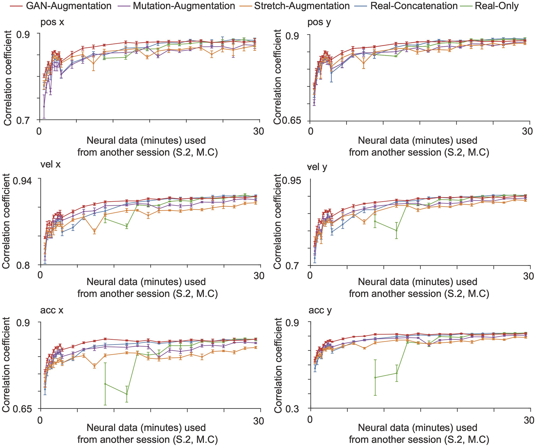
The GAN-augmentation, mutation-augmentation, stretch-augmentation, real-concatenation and real-only methods are shown in red, purple, orange, blue and green curves with an error bar in 5-fold cross-validation. The horizontal axis is the number of minutes of neural data from the session two of Monkey C used. The vertical axis is correlation coefficient between the decoded kinematics and real kinematics on an independent test set from the session two of Monkey C (mean + / − S.D., n = 5 folds). Synthesized spike trains that capture the neural attributes accelerate the training of a BCI decoder for the cross-session decoding.
ED Fig. 3. Cross-subject decoding.
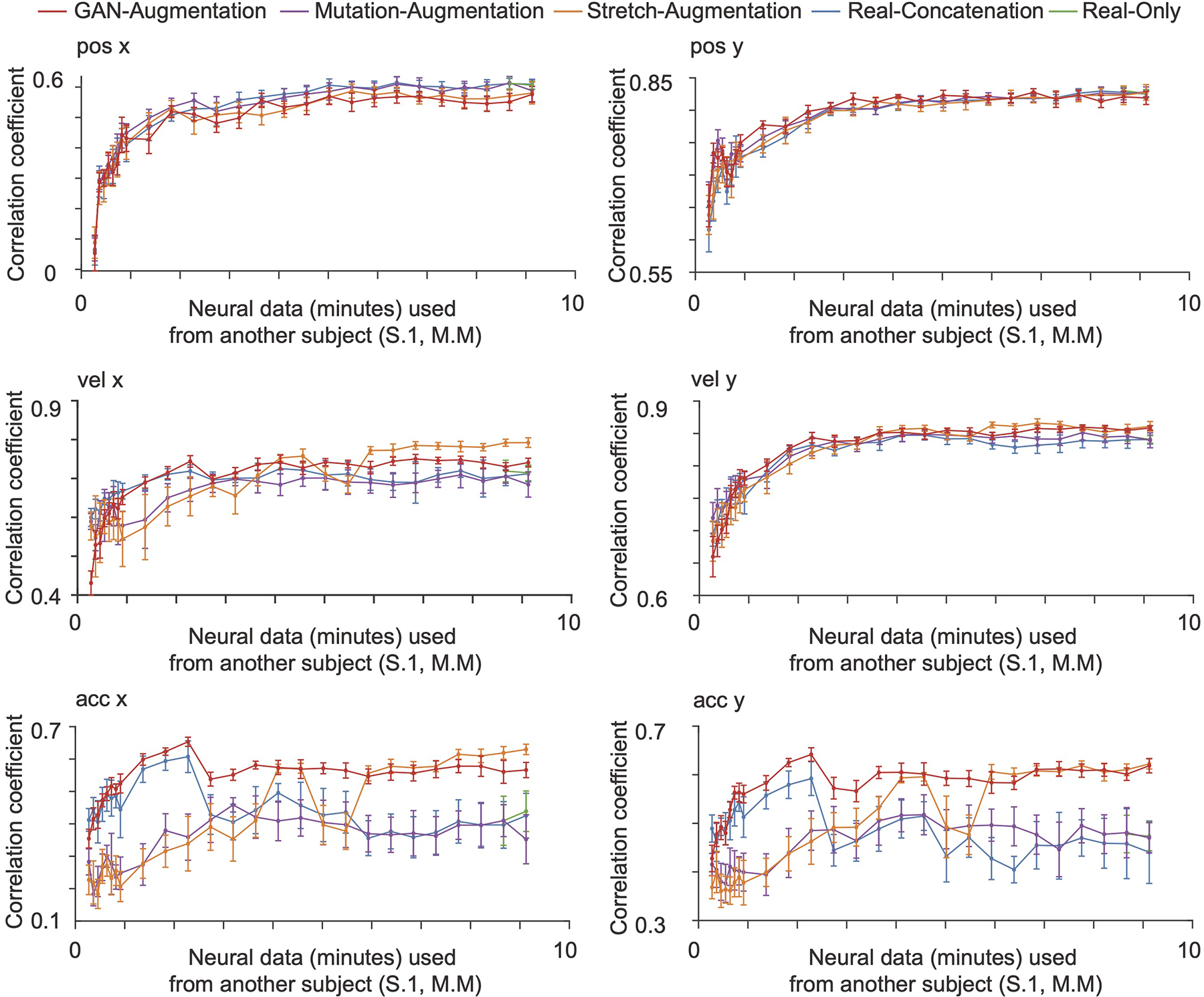
The GAN-augmentation, mutation-augmentation, stretch-augmentation, real-concatenation and real-only methods are shown in red, purple, orange, blue and green curves with an error bar in 5-fold cross-validation. The horizontal axis is the number of minutes of neural data from Monkey M used. The vertical axis is the correlation coefficient between the decoded kinematics and real kinematics on an independent test set from the Monkey M (mean + / − S.D., n = 5 folds). When the neural data from another subject is limited, synthesized spike trains that capture the neural attributes improve the cross-subject decoding performance on acceleration. Even with ample neural data for both subjects, the neural attributes learned from one subject can transfer some useful knowledge that improves the best achievable decoding performance on the acceleration of another subject.
ED Fig. 4.
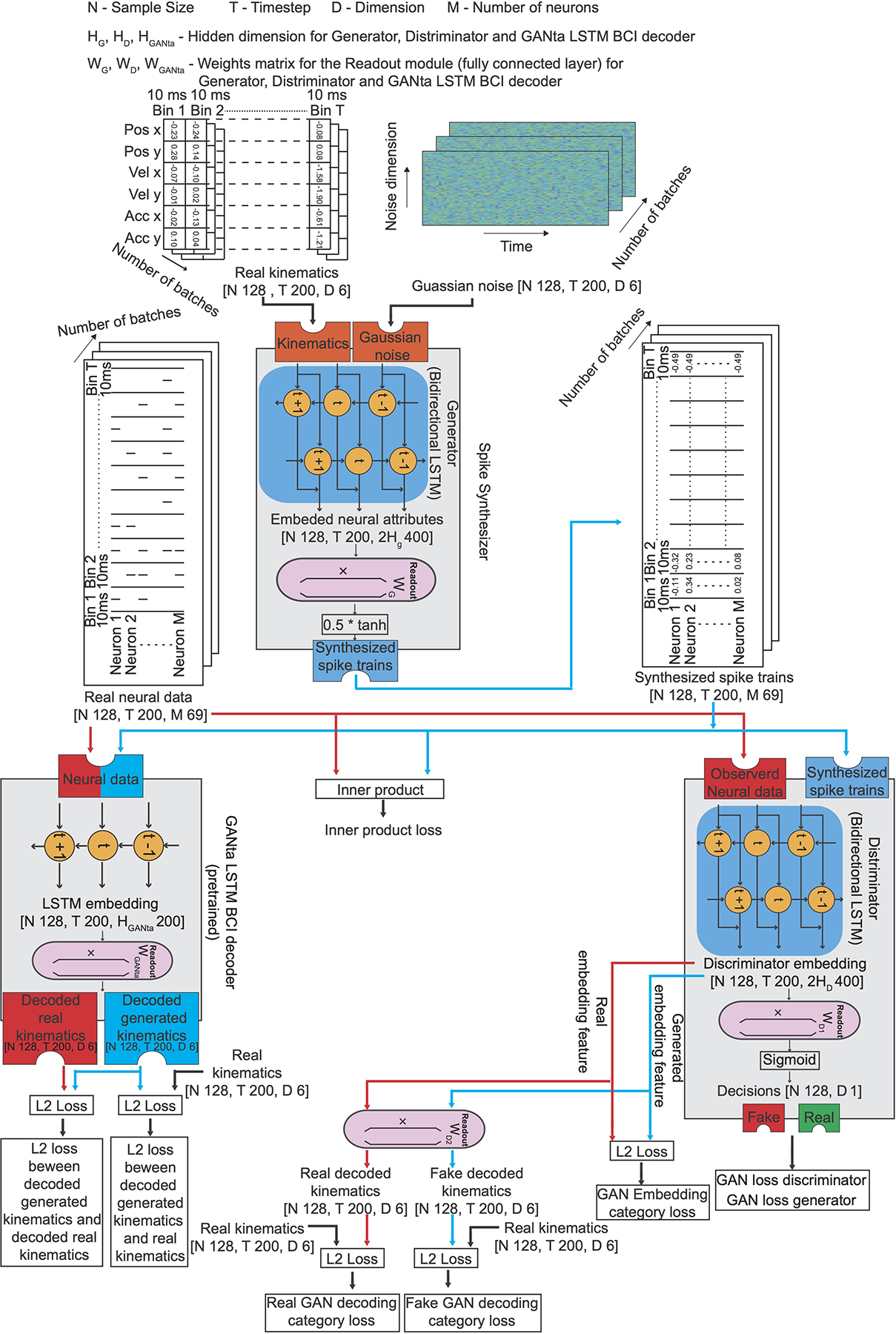
Detailed structure of the CC-LSTM-GAN.
ED Fig. 5. Averaged performance for cross-session decoding (11.73 minutes of neural data from S.2, M.C, which is the amount required for real-only to achieve good performance) on GAN-augmentation (red curve) and real-only (green curve) methods with increasing number of dropped neurons.
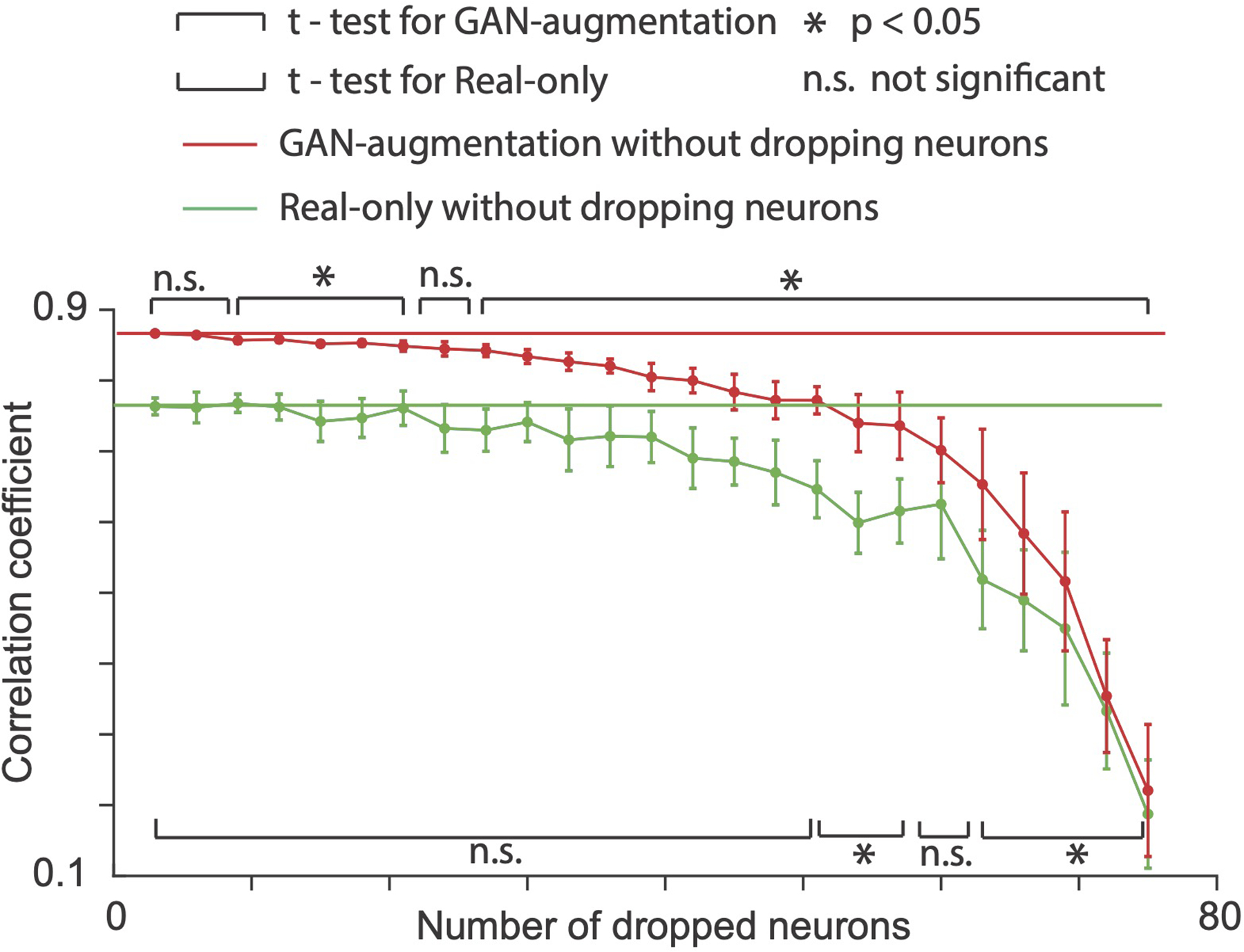
We randomly dropped neurons each time and repeated 10 times for each number of dropped neurons (mean + / − S.D., sample number = 10). P-values (t-test) for the GAN-augmentation method for all data points from left to right are [0.577, 0.130, 0.035, 0.040, 0.002, 0.012, 0.030, 0.054, 0.018, 0.009, 0.010, 0.001, 0.012, 0.004, 0.010, 0.006, 0.001, 0.014, 0.026, 0.007, 0.027, 0.011, 0.007, 0.0001, 9.74 * 10−5]. P-values for the real-only method for all data points from left to right are [0.973, 0.933, 0.774, 0.948, 0.487, 0.576, 0.909, 0.396, 0.306, 0.458, 0.326, 0.368, 0.279, 0.135, 0.050, 0.081, 0.021, 0.005, 0.012, 0.122, 0.008, 0.005, 0.0214, 0.0007, 5.17 * 10−5].
Supplementary Material
Acknowledgements
This work was supported by the National Science Foundation (grant number CCF-1317433), C-BRIC (one of six centers in JUMP, a Semiconductor Research Corporation (SRC) program sponsored by DARPA), the Intel Corporation and the National Institute of Health (grant number NIH NINDS T32 HD07418, F31 NS092356, NS053603 and NS074044). The authors affirm that the views expressed herein are solely their own, and do not represent the views of the United States government or any agency thereof.
Footnotes
Code availability
The codes used in this study are available in Github at https://github.com/shixianwen/Rapid-transfer-of-brain-machine-interfaces-to-new-neuronal-ensembles-or-participants.
Competing interests
The authors declare no competing interests.
Data availability
The raw and analysed datasets generated during the study are available in Github at https://github.com/shixianwen/Rapid-transfer-of-brain-machine-interfaces-to-new-neuronal-ensembles-or-participants.
References
- 1.Wessberg J et al. Real-time prediction of hand trajectory by ensembles of cortical neurons in primates. Nature (2000) doi: 10.1038/35042582. [DOI] [PubMed] [Google Scholar]
- 2.Velliste M, Perel S, Spalding MC, Whitford AS & Schwartz AB Cortical control of a prosthetic arm for self-feeding. Nature (2008) doi: 10.1038/nature06996. [DOI] [PubMed] [Google Scholar]
- 3.Taylor DM, Tillery SIH & Schwartz AB Direct cortical control of 3D neuroprosthetic devices. Science (80-. ). (2002) doi: 10.1126/science.1070291. [DOI] [PubMed] [Google Scholar]
- 4.Wessberg J et al. Real-time prediction of hand trajectory by ensembles of cortical neurons in primates. Nature (2000) doi: 10.1038/35042582. [DOI] [PubMed] [Google Scholar]
- 5.Carmena JM et al. Learning to control a brain-machine interface for reaching and grasping by primates. PLoS Biol. (2003) doi: 10.1371/journal.pbio.0000042. [DOI] [PMC free article] [PubMed] [Google Scholar]
- 6.Li Z et al. Unscented Kalman filter for brain-machine interfaces. PLoS One (2009) doi: 10.1371/journal.pone.0006243. [DOI] [PMC free article] [PubMed] [Google Scholar]
- 7.Wu W et al. Neural Decoding of Cursor Motion Using a Kalman Filter. Adv. Neural Inf. Process. Syst. 15 Proc. 2002 Conf. (2003) doi:10.1.1.6.8776. [Google Scholar]
- 8.Brockwell AE Recursive Bayesian Decoding of Motor Cortical Signals by Particle Filtering. J. Neurophysiol (2004) doi: 10.1152/jn.00438.2003. [DOI] [PubMed] [Google Scholar]
- 9.Gao Y, Black MJ, Bienenstock E, Wu W & Donoghue JP A quantitative comparison of linear and non-linear models of motor cortical activity for the encoding and decoding of arm motions. in International IEEE/EMBS Conference on Neural Engineering, NER (2003). doi: 10.1109/CNE.2003.1196789. [DOI] [Google Scholar]
- 10.Eden UT, Frank LM, Barbieri R, Solo V & Brown EN Dynamic Analysis of Neural Encoding by Point Process Adaptive Filtering. Neural Comput. (2004) doi: 10.1162/089976604773135069. [DOI] [PubMed] [Google Scholar]
- 11.Eden UT Point process adaptive filters for neural data analysis: Theory and applications. in Proceedings of the IEEE Conference on Decision and Control (2007). doi: 10.1109/CDC.2007.4434708. [DOI] [Google Scholar]
- 12.Hochreiter S & Schmidhuber J Long Short-Term Memory. Neural Comput. (1997) doi: 10.1162/neco.1997.9.8.1735. [DOI] [PubMed] [Google Scholar]
- 13.Glaser Joshua I and Chowdhury Raeed H and Perich Matthew G and Miller Lee E and Kording KP Machine learning for neural decoding. in arXiv preprint arXiv:1708.00909 (2017). [DOI] [PMC free article] [PubMed] [Google Scholar]
- 14.Moeendarbary E et al. The soft mechanical signature of glial scars in the central nervous system. Nat. Commun (2017) doi: 10.1038/ncomms14787. [DOI] [PMC free article] [PubMed] [Google Scholar]
- 15.Kozai TDY, Jaquins-Gerstl AS, Vazquez AL, Michael AC & Cui XT Brain tissue responses to neural implants impact signal sensitivity and intervention strategies. ACS Chem. Neurosci (2015) doi: 10.1021/cn500256e. [DOI] [PMC free article] [PubMed] [Google Scholar]
- 16.Duffau H Brain Plasticity and Reorganization Before, During, and After Glioma Resection. in Glioblastoma (2016). doi: 10.1016/B978-0-323-47660-7.00018-5. [DOI] [Google Scholar]
- 17.Tkach D, Reimer J & Hatsopoulos NG Observation-based learning for brain-machine interfaces. Current Opinion in Neurobiology (2008) doi: 10.1016/j.conb.2008.09.016. [DOI] [PMC free article] [PubMed] [Google Scholar]
- 18.Gallego JA, Perich MG, Chowdhury RH, Solla SA & Miller LE A stable, long-term cortical signature underlying consistent behavior. bioRxiv (2018) doi: 10.1101/447441. [DOI] [PMC free article] [PubMed] [Google Scholar]
- 19.Gao P et al. A theory of multineuronal dimensionality, dynamics and measurement. bioRxiv (2017) doi: 10.1101/214262. [DOI] [Google Scholar]
- 20.Pandarinath C et al. Inferring single-trial neural population dynamics using sequential auto-encoders. Nat. Methods (2018) doi: 10.1038/s41592-018-0109-9. [DOI] [PMC free article] [PubMed] [Google Scholar]
- 21.Farshchian A, Gallego JA, Cohen JP, et al. Adversarial Domain Adaptation for Stable Brain-Machine Interfaces. in (2019).
- 22.Sussillo D, Stavisky SD, Kao JC, Ryu SI & Shenoy KV Making brain-machine interfaces robust to future neural variability. Nat. Commun (2016) doi: 10.1038/ncomms13749. [DOI] [PMC free article] [PubMed] [Google Scholar]
- 23.Degenhart Alan D and Bishop William E and Oby Emily R and Tyler-Kabara Elizabeth C and Chase Steven M and Batista Aaron P and Byron MY Stabilization of a brain--computer interface via the alignment of low-dimensional spaces of neural activity. Nat. Biomed. Eng 1––14 (2020). [DOI] [PMC free article] [PubMed] [Google Scholar]
- 24.Gerstner W, Kistler WM, Naud R & Paninski L Neuronal dynamics: From single neurons to networks and models of cognition. Neuronal Dynamics: From Single Neurons to Networks and Models of Cognition (2014). doi: 10.1017/CBO9781107447615. [DOI]
- 25.Goodfellow Ian J., Pouget-Abadie* Jean, Mirza Mehdi, Xu Bing, Warde-Farley David, Ozair† Sherjil, Aaron Courville, Y. B. Generative Adversarial Nets Ian. Vet. Immunol. Immunopathol (2013) doi: 10.1016/j.vetimm.2013.08.005. [DOI] [Google Scholar]
- 26.Wei L, Hu L, Kim V, Yumer E & Li H Real-Time Hair Rendering Using Sequential Adversarial Networks. in Lecture Notes in Computer Science (including subseries Lecture Notes in Artificial Intelligence and Lecture Notes in Bioinformatics) (2018). doi: 10.1007/978-3-030-01225-0_7. [DOI] [Google Scholar]
- 27.Jetchev N & Bergmann U The Conditional Analogy GAN: Swapping Fashion Articles on People Images. in Proceedings - 2017 IEEE International Conference on Computer Vision Workshops, ICCVW 2017 (2018). doi: 10.1109/ICCVW.2017.269. [DOI] [Google Scholar]
- 28.Goodfellow I Generative Modeling Generative Modeling. NIPS (2016) doi: 10.1001/jamainternmed.2016.8245. [DOI] [Google Scholar]
- 29.Mirza M & Osindero S CGAN. CoRR (2014) doi: 10.1017/CBO9781139058452. [DOI] [Google Scholar]
- 30.Odena Augustus and Olah Christopher and Shlens J. Conditional image synthesis with auxiliary classifier gans. (2017).
- 31.Dai W, Yang Q, Xue G-R & Yu Y Boosting for transfer learning. in Proceedings of the 24th international conference on Machine learning - ICML ‘07 (2007). doi: 10.1145/1273496.1273521. [DOI] [Google Scholar]
- 32.Arnold A, Nallapati R & Cohen WW A comparative study of methods for transductive transfer learning. in Proceedings - IEEE International Conference on Data Mining, ICDM (2007). doi: 10.1109/ICDMW.2007.109. [DOI] [Google Scholar]
- 33.Lin Min, Chen Qiang, Y. S Network in network. (2013).
- 34.Ho Daniel, Liang Eric, Stoica Ion, Abbeel Pieter, C. X Population Based Augmentation: Efficient Learning of Augmentation Policy Schedules. in ICML (2019). [Google Scholar]
- 35.Tchumatchenko T, Geisel T, Volgushev M & Wolf F Spike correlations - What can they tell about synchrony? Frontiers in Neuroscience (2011) doi: 10.3389/fnins.2011.00068. [DOI] [PMC free article] [PubMed] [Google Scholar]
- 36.Dyer EL et al. A cryptography-based approach for movement decoding. Nat. Biomed. Eng (2017) doi: 10.1038/s41551-017-0169-7. [DOI] [PMC free article] [PubMed] [Google Scholar]
- 37.Ijspeert AJ, Nakanishi J, Hoffmann H, Pastor P & Schaal S Dynamical movement primitives: Learning attractor models formotor behaviors. Neural Computation (2013) doi: 10.1162/NECO_a_00393. [DOI] [PubMed] [Google Scholar]
- 38.Schaal S Dynamic Movement Primitives -A Framework for Motor Control in Humans and Humanoid Robotics. Adapt. Motion Anim. Mach (2006). [Google Scholar]
- 39.Poggio T & Bizzi E Generalization in vision and motor control. Nature (2004) doi: 10.1038/nature03014. [DOI] [PubMed] [Google Scholar]
- 40.Nuyujukian P et al. Performance sustaining intracortical neural prostheses. J. Neural Eng (2014) doi: 10.1088/1741-2560/11/6/066003. [DOI] [PubMed] [Google Scholar]
- 41.Thoroughman KA & Shadmehr R Learning of action through adaptive combination of motor primitives. Nature (2000) doi: 10.1038/35037588. [DOI] [PMC free article] [PubMed] [Google Scholar]
- 42.Stroud JP, Porter MA, Hennequin G & Vogels TP Motor primitives in space and time via targeted gain modulation in cortical networks. Nat. Neurosci (2018) doi: 10.1038/s41593-018-0276-0. [DOI] [PMC free article] [PubMed] [Google Scholar]
- 43.Shankar T, Pinto L, Tulsiani S & Gupta A DISCOVERING MOTOR PROGRAMS BY RECOMPOSING DEMONSTRATIONS. in ICLR 2020 (2020). [Google Scholar]
- 44.Costa RM, Ganguly K, Costa RM & Carmena JM Emergence of Coordinated Neural Dynamics Underlies Neuroprosthetic Learning and Skillful Control. Neuron (2017) doi: 10.1016/j.neuron.2017.01.016. [DOI] [PubMed] [Google Scholar]
- 45.Golub MD et al. Learning by neural reassociation. Nat. Neurosci (2018) doi: 10.1038/s41593-018-0095-3. [DOI] [PMC free article] [PubMed] [Google Scholar]
- 46.Sadtler PT et al. Neural constraints on learning. Nature (2014) doi: 10.1038/nature13665. [DOI] [PMC free article] [PubMed] [Google Scholar]
- 47.Gold JI & Shadlen MN The Neural Basis of Decision Making. Annu. Rev. Neurosci (2007) doi: 10.1146/annurev.neuro.29.051605.113038. [DOI] [PubMed] [Google Scholar]
- 48.Felsen G & Dan Y A natural approach to studying vision. Nature Neuroscience (2005) doi: 10.1038/nn1608. [DOI] [PubMed] [Google Scholar]
- 49.Paninski L, Pillow J & Lewi J Statistical models for neural encoding, decoding, and optimal stimulus design. Progress in Brain Research (2007) doi: 10.1016/S0079-6123(06)65031-0. [DOI] [PubMed] [Google Scholar]
- 50.Paninski L Superlinear Population Encoding of Dynamic Hand Trajectory in Primary Motor Cortex. J. Neurosci (2004) doi: 10.1523/JNEUROSCI.0919-04.2004. [DOI] [PMC free article] [PubMed] [Google Scholar]
- 51.LeCun YA, Bottou L, Orr GB & Müller KR Efficient backprop. Lect. Notes Comput. Sci. (including Subser. Lect. Notes Artif. Intell. Lect. Notes Bioinformatics) (2012) doi: 10.1007/978-3-642-35289-8-3. [DOI] [Google Scholar]
Associated Data
This section collects any data citations, data availability statements, or supplementary materials included in this article.
Supplementary Materials
Data Availability Statement
The raw and analysed datasets generated during the study are available in Github at https://github.com/shixianwen/Rapid-transfer-of-brain-machine-interfaces-to-new-neuronal-ensembles-or-participants.


