RNA promotes the formation of spatial compartments in the nucleus

SUMMARY

RNA, DNA, and protein molecules are highly organized within three-dimensional (3D) structures in the nucleus. Although RNA has been proposed to play a role in nuclear organization, exploring this has been challenging because existing methods cannot measure higher-order RNA and DNA contacts within 3D structures. To address this, we developed RNA & DNA SPRITE (RD-SPRITE) to comprehensively map the spatial organization of RNA and DNA. These maps reveal higher-order RNA-chromatin structures associated with three major classes of nuclear function: RNA processing, heterochromatin assembly, and gene regulation. These data demonstrate that hundreds of ncRNAs form high-concentration territories throughout the nucleus, that specific RNAs are required to recruit various regulators into these territories, and that these RNAs can shape long-range DNA contacts, heterochromatin assembly, and gene expression. These results demonstrate a mechanism where RNAs form high-concentration territories, bind to diffusible regulators, and guide them into compartments to regulate essential nuclear functions.

In Brief –

Mapping the proximity of RNAs to DNA and to other RNAs elucidates how cellular noncoding RNAs serve as spatial organizers controlling processes underpinning regulated gene expression.

Graphical Abstract

INTRODUCTION

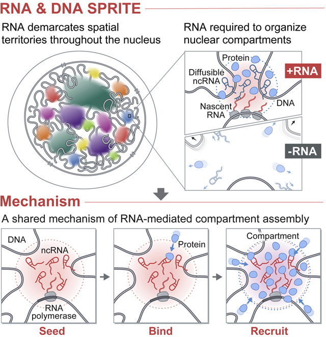
The nucleus is spatially organized in three-dimensional (3D) structures that are important for various functions including transcription and RNA processing (Dundr and Misteli, 2010; Pombo and Dillon, 2015; Strom and Brangwynne, 2019). To date, genome-wide studies of nuclear organization have focused primarily on the role of DNA (Dekker et al., 2017; Pombo and Dillon, 2015), yet nuclear structures are known to contain DNA, RNA, and protein molecules that are involved in shared functional and regulatory processes. These include classical compartments like the nucleolus (Pederson, 2011) (which contains transcribed ribosomal RNAs and their processing molecules) and nuclear speckles (Spector and Lamond, 2011) (which contain nascent pre-mRNAs and mRNA splicing components), as well as more recently described transcriptional condensates (which contain Mediator and RNA Pol II) (Cho et al., 2018; Guo et al., 2019). Because the complete molecular architecture of the nucleus has not been globally explored, the extent to which such compartments exist and contribute to nuclear function remains unknown. Even for the specific nuclear compartments that have been characterized, the mechanism by which intrinsically diffusible RNA and protein molecules become spatially organized remains unclear.

Nuclear RNA has long been proposed to play a central role in shaping nuclear structure (Nickerson et al., 1989; Rinn and Guttman, 2014). Over the past decade it has become clear that mammalian genomes encode thousands of nuclear-enriched ncRNAs (Frankish et al., 2019), several of which play critical regulatory roles (Rinn and Chang, 2012). These include ncRNAs involved in splicing of pre-mRNAs (snRNAs) (Black, 2003; Nilsen and Graveley, 2010), cleavage and modification of pre-ribosomal RNAs (snoRNAs, Rnase MRP) (Kiss-László et al., 1996; Watkins and Bohnsack, 2012), 3’-end cleavage and processing of the non-polyadenylated histone pre-mRNAs (U7 snRNA) (Kolev and Steitz, 2005), and transcriptional regulation (e.g. Xist (Plath et al., 2002) and 7SK (Egloff et al., 2018)). Many of these ncRNAs localize within specific compartments in the nucleus (Dundr and Misteli, 2010). For example, snoRNAs and the 45S pre-ribosomal RNA localize within the nucleolus (Pederson, 2011), the Xist lncRNA localizes on the inactive X chromosome (Barr body) (Engreitz et al., 2013), and snRNAs and Malat1 localize within nuclear speckles (Tripathi et al., 2010).

In each of these examples, RNA, DNA, and protein components simultaneously interact within precise structures. While the localization of specific ncRNAs have been well studied, the localization patterns of most nuclear ncRNAs remain unknown because no existing method can simultaneously measure higher-order RNA-RNA, RNA-DNA, and DNA-DNA contacts within 3D structures. As a result, it is unclear: (i) which specific RNAs are involved in nuclear organization, (ii) which nuclear compartments are dependent on RNA, and (iii) what mechanisms RNAs utilize to organize nuclear structures.

Microscopy is currently the only way to relate RNA and DNA molecules in 3D space, yet it is limited to examining a small number of components and requires a priori knowledge of which RNAs and nuclear structures to explore. An alternative approach is genomic mapping of RNA-DNA contacts using proximity-ligation methods (Bell et al., 2018; Bonetti et al., 2019; Li et al., 2017; Sridhar et al., 2017; Yan et al., 2019). While these can provide genome-wide pairwise maps of RNA-DNA interactions, they do not provide information about the 3D organization of these molecules. Moreover, we recently showed that proximity-ligation methods can fail to identify pairwise contacts between molecules if they are not close enough in space to be directly ligated (Quinodoz et al., 2018). Consistent with this, existing methods fail to identify known RNA-DNA contacts within nuclear bodies including nucleoli, histone locus bodies, and Cajal bodies (Bonetti et al., 2019; Sridhar et al., 2017; Yan et al., 2019).

We recently developed SPRITE, which utilizes split-and-pool barcoding to generate comprehensive and multi-way 3D maps of the nucleus across a wide range of distances (Quinodoz et al., 2018). We showed that SPRITE accurately maps the spatial organization of DNA arranged around two nuclear bodies – nucleoli and nuclear speckles. However, our original version could not detect the majority of RNAs, including low abundance ncRNAs known to organize within several well-defined nuclear structures. Here, we introduce a dramatically improved method, RNA & DNA SPRITE (RD-SPRITE), which enables simultaneous, high-resolution mapping of thousands of RNAs, including low abundance RNAs such as individual nascent pre-mRNAs and ncRNAs, relative to all other RNA and DNA molecules in 3D space. Using this approach, we identify several higher-order RNA-chromatin hubs and hundreds of ncRNAs that form high concentration territories throughout the nucleus. Focusing on specific examples, we show that many of these RNAs recruit diffusible ncRNA and protein regulators and can shape long-range DNA contacts, heterochromatin assembly, and gene expression within these territories. Together, our results highlight a role for RNA in the formation of compartments involved in essential nuclear functions including RNA processing, heterochromatin assembly, and gene regulation.

RESULTS

RD-SPRITE generates accurate maps of higher-order RNA and DNA contacts

To explore the role of RNA in shaping nuclear structure, we improved the efficiency of the RNA-tagging steps of our SPRITE method (Quinodoz et al., 2018) to enable detection of all classes of RNA (see Methods). We refer to this new approach as RNA & DNA SPRITE (RD-SPRITE). It works as follows: (i) RNA, DNA, and protein contacts are crosslinked to preserve their spatial relationships in situ, (ii) cells are lysed and the contents fragmented into smaller complexes, (iii) molecules within each complex are tagged with an RNA or DNA-specific adaptor, (iv) barcoded using an iterative split-and-pool strategy to uniquely assign a shared barcode to all DNA and RNA components contained within a complex, (v) DNA and RNA are sequenced, and (vi) all reads sharing identical barcodes are merged into a SPRITE cluster (Figure 1A, S1A–B). Because RD-SPRITE does not rely on proximity ligation, it can detect multiple RNA and DNA molecules that associate simultaneously.

Figure 1: RD-SPRITE generates maps of higher-order RNA and DNA contacts.

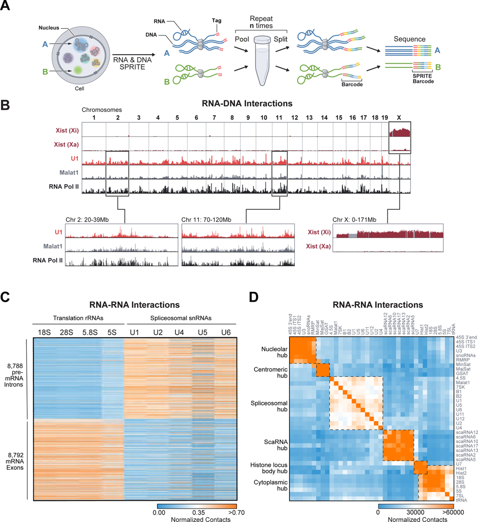
(A) Schematic of RD-SPRITE: Crosslinked cells are fragmented, DNA and RNA are barcoded through multiple rounds of split-and-pool barcoding, and SPRITE clusters defined as a group of molecules sharing a barcode. (B) Xist unweighted contacts on the inactive (Xi) or active X chromosome (Xa), U1 and Malat1 weighted contacts, and RNA Pol II (ENCODE) across the genome. Gray demarcates masked regions. (C) Heatmap showing unweighted RNA-RNA contacts between translation-associated RNAs or splicing RNAs (columns) and introns or exons of mRNAs (rows). (D) Heatmap of unweighted RNA-RNA contact frequencies for several classes of RNA. Boxes denote hubs. See also Figure S1 and Table S1.

We performed RD-SPRITE in an F1 hybrid female mouse ES cell line engineered to induce Xist from a single allele. We sequenced libraries on a NovaSeq S4 run to generate ~8 billion reads corresponding to ~720 million SPRITE clusters (Figure S1C, Table S2–3). To ensure that RD-SPRITE accurately measures bona fide RNA interactions, we focused on RNA-DNA contacts for several ncRNAs that were previously mapped to chromatin and reflect a range of known cis and trans localization patterns. We observed strong enrichment of: (i) Xist over the inactive X (Xi), but not the active X chromosome (Xa) (Figure 1B, S1D) (Engreitz et al., 2013); (ii) Malat1 and U1 over actively transcribed Pol II genes (Figure 1B) (Engreitz et al., 2014; West et al., 2014); and (iii) telomerase RNA component (Terc) over telomere-proximal regions of all chromosomes (Figure S1E) (Mumbach et al., 2019; Schoeftner and Blasco, 2008).

Next, we focused on known RNA-RNA contacts in different cellular locations. We observed a large number of contacts between translation-associated RNAs in the cytoplasm, including all RNA components of the ribosome and ~8000 individual mRNAs (exons), but not with pre-mRNAs (introns) (Figure 1C). Conversely, we observed many contacts between snRNA components of the spliceosome and individual pre-mRNAs (introns) in the nucleus (Figure 1C).

Together, these results demonstrate that RD-SPRITE accurately measures RNA-DNA and RNA-RNA contacts in the nucleus and cytoplasm. While we focus primarily on contacts within the nucleus, RD-SPRITE can also be utilized to study RNA compartments beyond the nucleus (Banani et al., 2017).

Multiple ncRNAs co-localize within spatial compartments in the nucleus

To explore which RNAs localize within spatial compartments, we first mapped pairwise RNA-RNA and RNA-DNA contacts and identified several groups of RNAs that display high pairwise contact frequencies with each other, but low contact frequencies with RNAs in other groups (Figure 1D). Interestingly, the multiple pairwise interacting RNAs within the same group localize to similar genomic DNA regions (Figure S1G–H). Using a combination of RNA FISH and immunofluorescence (IF), we confirmed that RNAs within a group co-localize (Figure S1I) while RNAs in distinct groups localize to different regions of the cell (Figure S1J).

We next explored whether groups of pairwise interacting RNAs simultaneously associate within higher-order structures. To do this, we compared the frequency of contacts between 3 or more distinct RNAs to the expected frequency if these RNAs were randomly distributed. We observed many significant multi-way contacts between RNAs within each group (Table S1). Overall, we observed a significantly higher number of multi-way contacts among RNAs within a group than between RNAs from distinct groups (~50-fold for 3-way contacts, Figure S1F). Because these groups of RNAs are found in higher-order structures, we refer to them as “hubs” and explore them below.

ncRNAs form processing hubs around genomic DNA encoding their nascent targets

We first explored the RNA-DNA hubs associated with RNA processing. Specifically, we examined the RNAs within these hubs (RNA-RNA interactions), their location relative to genomic DNA (RNA-DNA interactions), and the 3D organization of these DNA loci (DNA-DNA interactions).

(i). ncRNAs involved in ribosomal RNA processing organize around transcribed ribosomal RNA genes.

We identified a hub that includes the 45S pre-ribosomal RNA, RNase MRP, and dozens of snoRNAs involved in rRNA biogenesis (Figure 1D, S2A). rRNA is transcribed as a single 45S precursor RNA, is cleaved by RNAse MRP, and is modified by various snoRNAs to generate the mature 18S, 5.8S, and 28S rRNAs (Baßler and Hurt, 2019). We found that these ncRNAs form multi-way contacts with each other (p<0.01, z-score=31, Table S1) and localize at genomic locations proximal to ribosomal DNA repeats that encode the 45S pre-rRNA and other genomic regions that organize around the nucleolus (Quinodoz et al., 2018) (Figure 2A, S2B). We explored the DNA-DNA interactions that occur within SPRITE clusters containing multiple nucleolar hub RNAs and observed that these RNAs and genomic DNA regions are organized together in 3D space (Figure 2B, S2C). Our results demonstrate that the nascent 45S pre-rRNA, along with the diffusible snoRNAs and RNase MRP, are spatially enriched near the DNA loci from which rRNA is transcribed.

Figure 2: Non-coding RNAs involved in RNA processing organize within hubs.

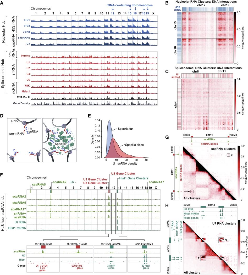
(A) Weighted RNA-DNA contacts (1Mb resolution) for several RNAs within the nucleolar and spliceosomal hubs are plotted alongside Pol II occupancy (ENCODE) and gene density. Chromosomes with rDNA are shown in blue. (B) Weighted DNA-DNA contacts in SPRITE clusters containing nucleolar hub RNAs are shown between chromosomes 12+19 and 15+16. Blue/white color bar represents high and low 45S RNA-DNA contacts. (C) Weighted DNA-DNA contacts in SPRITE clusters containing spliceosomal hub RNAs are shown between chromosomes 4 and 8+11. Red/white color bar represents U1 RNA-DNA contacts. (D) Illustration of two possible snRNA localization models: (left) localization occurs primarily through association with nascent pre-mRNAs; (right) localization depends on 3D position of an individual gene. (E) U1 snRNA density over genomic DNA regions with comparable expression levels that are close (red) or far (blue) from nuclear speckles. (F) Weighted RNA-DNA contacts for clusters containing various scaRNAs or scaRNAs and snRNAs (green) or U7 and histone pre-mRNAs (teal). (G) Weighted DNA-DNA contacts across a genomic region containing snRNA genes for all (bottom) or scaRNA-containing (top) SPRITE clusters. scaRNA RNA-DNA contacts are shown along the top and side axes and enriched loci highlighted by black box and arrow. (H) Weighted DNA-DNA contacts in a genomic region containing histone genes for all (bottom) or U7-containing (top) SPRITE clusters. U7 and histone pre-mRNA RNA-DNA contacts are shown along the top and side axis and enriched loci marked with black box and arrow. See also Figure S2.

(ii). ncRNAs involved in mRNA splicing are spatially concentrated around genes containing a high density of Pol II.

We identified a hub that contains nascent pre-mRNAs, major and minor spliceosomal ncRNAs, and other ncRNAs associated with transcriptional regulation and mRNA splicing (Figure 1D, Table S1). Nascent pre-mRNAs are known to be directly bound and cleaved by spliceosomal RNAs to generate mature mRNA transcripts (Lee and Rio, 2015), yet it is unclear how spliceosomal RNAs are organized in the nucleus relative to target pre-mRNAs and genomic DNA (Bentley, 2014; Herzel et al., 2017). We first explored the possibility that the localization of splicing RNAs to genomic DNA regions occurs primarily through their association with nascent pre-mRNAs. In this case, we would expect the DNA occupancy of splicing RNAs to be proportional to mRNA transcription levels, regardless of the 3D position of an individual gene in the nucleus. However, we find that splicing RNAs do not show a uniform occupancy over all genes but are more highly enriched over DNA regions containing a high-density of actively transcribed Pol II genes (r = 0.86–0.90, Figure 2A, S2B,D). When we explored the higher-order DNA contacts of these RNAs, we found that these genomic DNA regions form preferential inter-chromosomal contacts and are comparable to regions organized around nuclear speckles (Quinodoz et al., 2018) (Figure 2C, S2E). We observed that snRNA localization was significantly higher over DNA regions that are close to the nuclear speckle relative to those located farther away (Figure 2D), even when focusing on genes with comparable levels of transcription (Figure 2E). These results demonstrate that spliceosomal RNAs are spatially enriched near clusters of actively transcribed Pol II genes and their associated nascent pre-mRNAs.

(iii). ncRNAs involved in snRNA biogenesis are organized around snRNA gene clusters.

We identified a hub containing several small Cajal body-associated RNAs (scaRNAs) and snRNAs (Figure 1D, Table S1, Figure S2F). snRNAs are Pol II transcripts produced from multiple locations throughout the genome that undergo 2’-O-methylation and pseudouridylation before acting as functional components of the spliceosome at thousands of nascent pre-mRNA targets (Tycowski et al., 1998). scaRNAs directly hybridize to snRNAs to guide these modifications (Darzacq et al., 2002). We found that scaRNAs are highly enriched at discrete genomic regions containing multiple snRNA genes in close linear space (Figure 2F). Although we cannot directly distinguish between the spatial localization of nascent snRNAs and mature snRNAs, we found that SPRITE clusters containing snRNAs and scaRNAs are highly enriched at genomic DNA regions containing snRNA genes (Figure 2F), indicating that nascent snRNAs are enriched near their transcriptional loci. Despite being separated by large genomic distances, these DNA regions form long-range contacts (Figure 2G) and scaRNAs, snRNAs, and their associated DNA loci simultaneously interact within higher-order SPRITE clusters (Figure S2G). These results demonstrate that these components simultaneously interact within a spatial compartment in the nucleus. We note that this snRNA biogenesis hub may be similar to Cajal bodies, which have been noted to contain snRNA genes and scaRNAs (Machyna et al., 2013) (Figure S2J). However, Cajal bodies are traditionally defined by the presence of Coilin foci in the nucleus (Machyna et al., 2015; Nizami et al., 2010; Ogg and Lamond, 2002) and based on this definition, our mES cells do not contain visible Cajal bodies (Figure S2L). Despite the absence of traditionally defined Cajal bodies, our data suggest that snRNA biogenesis hubs do indeed exist and form around snRNA gene loci, even in the absence of observable Coilin foci.

(iv). The histone processing U7 snRNA is enriched around histone gene loci.

We identified a hub containing U7 and various histone mRNAs (Figure 1D). Unlike most pre-mRNAs, histone pre-mRNAs are not polyadenylated; their 3’ends are bound and cleaved by the U7 snRNP complex to produce mature histone mRNAs (Marzluff and Koreski, 2017; Marzluff et al., 2008). This process is thought to occur within nuclear structures called Histone Locus Bodies (HLBs) (Nizami et al., 2010), demarcated by NPAT protein (Figure S2H). We observed that U7 localizes at genomic DNA regions containing histone mRNA genes, specifically at two histone gene clusters on chromosome 13 (Figure 2F). To determine whether U7, histone genes, and histone pre-mRNAs spatially co-occur, we focused on DNA-DNA contacts from U7-containing clusters and observed long-range DNA contacts between the two histone gene clusters on chromosome 13 (Figure 2H). Consistent with previous observations that HLBs and Cajal bodies are often adjacent to each other in the nucleus (Nizami et al., 2010), we observed that scaRNAs also localize to histone gene clusters, form higher-order DNA interactions, and are adjacent to the HLB in the nucleus (Figure 2F, S2G, S2I–L).

Together, these results indicate that higher-order spatial organization of diffusible regulators around shared DNA sites and their corresponding nascent RNA targets is a common feature of many forms of RNA processing.

RNA processing compartments are dependent on nascent RNA

In each of these examples, we observed spatial compartments that consist of: (i) nascent RNAs localized near their DNA loci, (ii) these DNA loci forming long-range 3D contacts, and (iii) diffusible ncRNAs associating with these nascent RNAs and DNA loci within the compartment. Because many of these diffusible ncRNAs are known to directly bind to the nascent RNA (e.g. snoRNAs bind 45S pre-rRNA (Jády and Kiss, 2001)), we hypothesized that nascent transcription of RNA might act to form a high-concentration territory at these genomic DNA sites and recruit these diffusible ncRNAs into these spatial compartments.

To test this, we treated cells with actinomycin D (ActD), a drug that inhibits RNA Pol I and Pol II transcription (Bensaude, 2011), for 4 hours and performed RD-SPRITE (Figure 3A, S3A). We confirmed that ActD treatment led to robust inhibition of various nascent RNAs (e.g. 45S, histone mRNAs), but did not impact the steady-state RNA levels of their associated diffusible ncRNAs (snoRNAs, U7, scaRNAs) (Figure 3B, S3B–C). Next, we explored the spatial organization of DNA and RNA. Strikingly, while we did not observe structural changes of most DNA structural features (e.g., chromosome territories, A/B compartments, Figure S3I), we observed large-scale disruption of DNA and RNA organization within the nuclear structures associated with ribosome, snRNA, and histone biogenesis.

Figure 3: Inhibition of nascent RNA transcription disrupts RNA processing hubs.

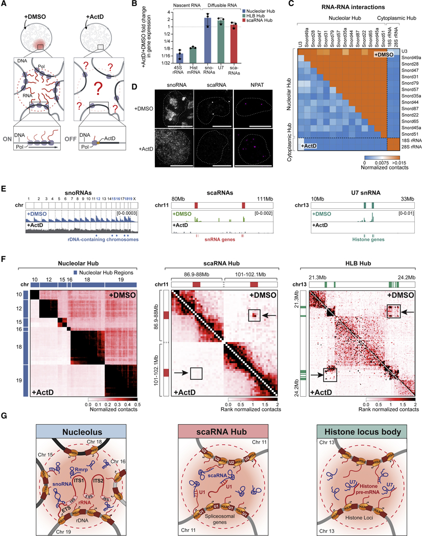
(A) Schematic of transcriptional inhibition of Pol I and Pol II in cells treated with Actinomycin D (+ActD) or control (+DMSO). (B) Gene expression changes of RNAs of interest following ActD treatment. Error bars represent standard deviation of 3 replicate experiments. (C) RNA-RNA contact frequency of snoRNAs and rRNAs following ActD (bottom) or DMSO (top) treatment. (D) Imaging of snoRNA, scaRNA, or NPAT protein upon ActD or DMSO treatment. Scalebar is 10μm. (E) RNA-DNA contacts upon DMSO (top) or ActD (bottom) treatment for aggregated snoRNAs (left, cluster size 1001–10000), scaRNAs (middle, weighted), and U7 (right, weighted). (F) DNA-DNA contact matrices upon ActD (bottom) or DMSO (top) treatment. (Left) Nucleolar-hub associated genomic regions (previously described in (Quinodoz et al., 2018)). (Middle) Two regions on chromosome 11 containing snRNA clusters. (Right) Region on chromosome 13 containing histone gene clusters. (Middle, Right) Rank normalized contacts are defined by rescaling contact frequency based on their rank-order to enable comparison between samples. (G) Model of how nascent transcription of RNA organizes diffusible ncRNAs and genomic DNA to form each hub. See also Figure S3.

Focusing on the nucleolar hub, we observed a strong depletion of RNA-RNA contacts between the various snoRNAs (Figure 3C) and global disruption of snoRNA localization at nucleolar DNA sites (Figure 3D–E, S3D) such that snoRNA and RMRP localization became diffusive throughout the nucleus (Figure 3D, S3E,H). We also observed a dramatic reduction in inter-chromosomal contacts between genomic DNA regions contained within the nucleolar hub (Figure 3F, S3G). These results indicate that transcription of 45S pre-rRNA (which is known to interact with snoRNAs and RNase MRP (Cech and Steitz, 2014; Goldfarb and Cech, 2017) acts to concentrate these diffusible ncRNAs and organize DNA loci into the nucleolar compartment (Figure 3G).

Similarly, ActD treatment led to a loss of focal localization of scaRNAs at snRNA genes (Figure 3E, S3D), a change from focal to diffusive localization throughout the nucleus (Figure 3D), and a striking reduction in the long-range DNA-DNA contacts between snRNA genes (Figure 3F, S3G). In addition, we observed a loss of focal localization of U7 at the histone genes (Figure 3E, S3D), loss of long-range DNA-DNA interactions between the histone loci (Figure 3F), and an increase in the number of nuclear foci containing HLB-associated proteins (NPAT) within each cell (Figure 3D, S3F). These results indicate that nascent transcription of snRNAs and histone pre-mRNAs is required to drive organization of these nuclear compartments (Figure 3G).

Although we did not observe major changes in DNA-DNA or RNA-DNA contacts within the splicing hub, this may be because ActD only led to a modest reduction (<2-fold) in nascent pre-mRNA (introns) levels (Figure S3A). Consistent with this, we previously observed significant changes in snRNA localization at active DNA sites following treatment with flavopiridol (FVP) (Engreitz et al., 2014), a transcriptional inhibitor that leads to robust reduction of nascent pre-mRNA levels.

Satellite-derived ncRNAs organize HP1 localization at inter-chromosomal hubs

In addition to RNA processing, we identified a hub containing ncRNAs transcribed from minor and major satellite DNA regions within centromeric and pericentromeric regions, respectively (Figure 1D). We found that these ncRNAs localize primarily over centromere-proximal regions (Figure 4A–B, S4B) and organize into higher-order structures containing these ncRNAs and multiple centromere-proximal regions from different chromosomes (Figure 4C, S4A). To confirm this, we performed DNA FISH on the major and minor satellite DNA and observed higher-order structures where multiple centromeres interact simultaneously (Figure 4D), indicating that satellite-derived ncRNAs demarcate nuclear compartments where centromeric regions from multiple chromosomes associate with each other.

Figure 4: Satellite-derived ncRNAs organize HP1 at inter-chromosomal hubs.

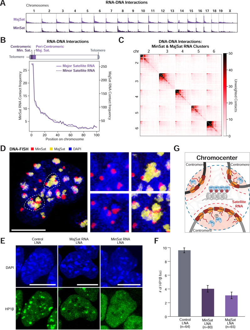
(A) Unweighted RNA-DNA contact frequencies of major and minor satellite-derived ncRNAs across the genome or (B) aggregated across all chromosomes. (C) Unweighted DNA-DNA contacts for chromosomes 2 – 6 within clusters containing a satellite-derived RNA. (D) DNA FISH of major (yellow) and minor (red) satellite DNA in the nucleus (DAPI, blue). Dashed lines demarcate the two DAPI-dense structures shown as zoom-ins on the right. Scalebar is 10μm. (E) HP1β IF following LNA-mediated knockdown of major (MajSat) and minor (MinSat) satellite-derived RNAs. Scalebar is 10μm. (F) Quantification of the mean number of HP1β foci per cell following LNA knockdown. n=number of cells analyzed, error bars represent standard error. (G) Schematic of Chromocenter Hub. Satellite RNAs are spatially concentrated (red gradient) near centromeric DNA. Individual centromeres assemble into a heterochromatic chromocenter structure highly enriched with HP1 protein. See also Figure S4.

Centromeric and pericentromeric DNA (chromocenters) are enriched for various heterochromatin enzymes and chromatin modifications, including the HP1 protein and H3K9me3 modifications (Maison et al., 2002). Previous studies have shown that global disruption of RNA by RNase A leads to disruption of HP1 localization at chromocenters (Maison et al., 2002). However, RNAse A is not specific and can impact several structures in the nucleus, including nucleoli (Barutcu et al., 2019). Because major and minor satellite-derived ncRNAs localize exclusively within centromere-proximal structures, we hypothesized that these ncRNAs might be important for HP1 localization. To test this, we used an antisense oligonucleotide (ASO) to degrade either the major or minor satellite RNAs (Figure S4C–D) and observed depletion of HP1 proteins over these centromere-proximal structures (Figure 4E–F, S4E) without impacting overall HP1 protein levels (Figure S4F). Because disruption of the major satellite RNAs also led to reduced minor satellite RNA levels (Figure S4C–D), we cannot exclude that altered HP1 localization is solely due to depletion of minor satellite RNA.

Our results demonstrate that satellite-derived ncRNAs are enriched close to their transcriptional loci and recruit HP1 into centromere-proximal nuclear compartments (Figure 4G). Consistent with this, previous studies have shown that disruption of the major satellite-derived RNA prior to the formation of chromocenters during preimplantation development leads to loss of chromocenter formation, lack of heterochromatin formation, and embryonic arrest (Casanova et al., 2013).

Hundreds of non-coding RNAs localize in spatial proximity to their transcriptional loci

Thousands of nuclear-enriched ncRNAs are expressed in mammalian cells, but only a handful have been mapped on chromatin. We mapped ~650 lncRNAs in ES cells and observed a striking difference in chromatin localization between these and mature mRNAs (Figure 5A, S5A–B, see Methods). Specifically, we found that the vast majority (93%) of the lncRNAs are strongly enriched within 3D proximity of their transcriptional loci (Figure 5B–D, S5C). This is consistent with previous microscopy measurements that showed that most lncRNAs measured form enriched foci in the nucleus (Cabili et al., 2015). In contrast, we find that mature mRNAs are depleted near their transcriptional loci and at all other genomic locations (chromatin enrichment score <0), consistent with their localization in the cytoplasm (Figure 5A, S5B,D–E). We observed a similar lack of chromatin enrichment for a subset of lncRNAs, including Norad which functions in the cytoplasm (Figure 5A–B) (Lee et al., 2016). Additionally, not all lncRNAs with high chromatin enrichment are restricted to the 3D territory around their locus. For example, Malat1 is strongly enriched on chromatin but localizes broadly across all chromosomes (Figure 5A–B, S5C).

Figure 5: Most lncRNAs localize at genomic targets in 3D proximity to their transcriptional loci.

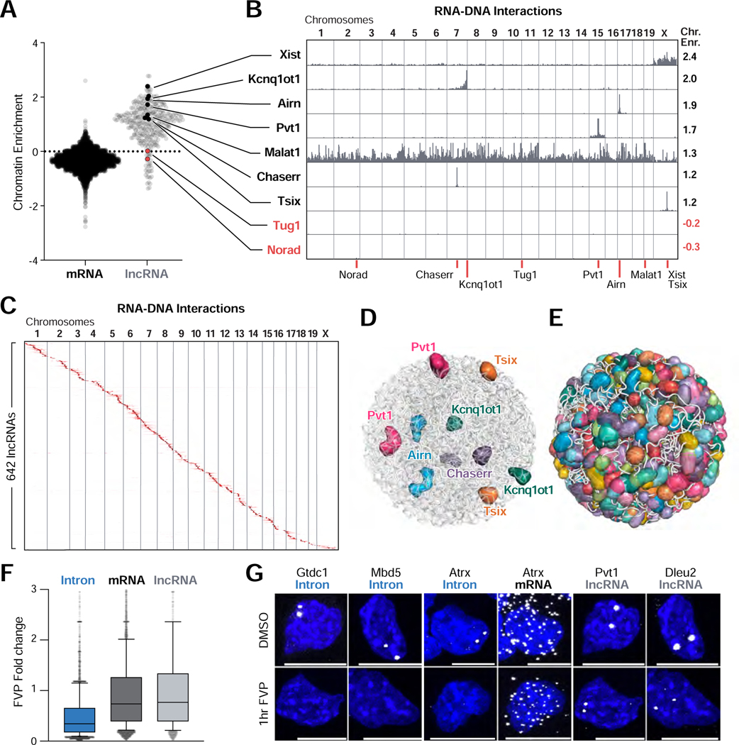
(A) Chromatin enrichment score for mRNAs and lncRNAs. Values > and < 0 represent RNAs enriched and depleted on chromatin, respectively. (B) Unweighted RNA-DNA localization maps for selected chromatin-enriched (black) and chromatin-depleted (red) lncRNAs. Chromatin enrichment scores (Chr. Enr.) are listed (right). Red lines (bottom) indicate transcriptional locus for each RNA. (C) Unweighted RNA-DNA localization map of 642 lncRNAs ordered by genomic position of their transcriptional loci. (D) 3D space filling nuclear structure model of the selected lncRNAs or (E) 543 lncRNAs that display at least 50-fold enrichment in the nucleus. Each sphere corresponds to a 1 Mb region or larger where an individual lncRNA is enriched. (F) Change in RNA levels between untreated and flavopiridol (FVP)-treated mouse ES cells (Jonkers et al., 2014) for introns, mRNAs, and lncRNAs. Plot: line represents median, box extends from 25^th to 75^th percentiles, and whiskers from 10^th to 90^th percentiles. (G) RNA FISH for selected introns, mRNA exons, and lncRNAs following FVP (bottom) or DMSO (top) treatment for 1 hour. Scalebar is 10μm. See also Figure S5.

Localization of lncRNAs in proximity to their transcriptional loci could represent either unstable RNA products transiently associated with their transcriptional loci prior to degradation (consistent with nascent pre-mRNA localization (Levesque and Raj, 2013)) or stable association of mature RNAs after transcription (Figure S5A). To test whether they represent transient RNA products, we measured the expression of lncRNAs after FVP treatment. We explored a previously published RNA sequencing experiment performed after 50 minutes of treatment with FVP in mES cells (Jonkers et al., 2014). Consistent with previous reports (Clark et al., 2012), we found that virtually all lncRNAs were dramatically more stable than nascent pre-mRNAs and comparable in stability to mature mRNAs (Figure 5F). To confirm this, we performed RNA FISH for 4 lncRNAs, 6 nascent pre-mRNAs (introns), and 1 mature mRNA (exons) in untreated cells and upon FVP treatment. We found that all of these lncRNAs form stable nuclear foci that are retained upon transcriptional inhibition (Figure 5G, S5F). In contrast, all nascent pre-mRNA foci are lost upon transcriptional inhibition, even though we observe no impact on their mature mRNA products (Figure 5G).

Together, these results demonstrate that many hundreds of lncRNAs form high concentration spatial territories throughout the nucleus (Figure 5E).

Non-coding RNAs guide regulatory proteins to nuclear territories to regulate gene expression

Because hundreds of lncRNAs are enriched in territories throughout the nucleus, we explored whether RNAs might impact protein localization within these territories. Recently, we and others showed that SHARP (also called Spen) directly binds Xist (Chu et al., 2015; McHugh et al., 2015) and recruits the HDAC3 histone deacetylase complex to the X chromosome to silence transcription (McHugh et al., 2015; Żylicz et al., 2019) Figure 6A, S6A). To explore the nuclear localization of SHARP more globally, we performed super-resolution microscopy and found two types of localization: low-level diffusive localization throughout the nucleus and compartmentalized localization within dozens of well-defined foci (~50–100 foci/nucleus; Figure 6B, Video S1). To determine whether the SHARP foci are dependent on RNA, we deleted the RNA binding domains from SHARP (ΔRRM) and visualized its localization (Figure 6A). We observed diffuse localization of the mutant protein and loss of all compartmentalized SHARP foci (Figure 6B, Video S2) even though there was no change in overall SHARP protein levels (Figure S6B). These results demonstrate that RNA is required for SHARP localization to dozens of spatial territories throughout the nucleus.

Figure 6: SHARP is enriched within dozens of RNA-mediated compartments in the nucleus and can regulate gene expression within specific compartments.

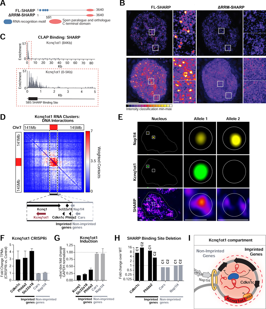
(A) Full length (FL) SHARP (also referred to as Spen) contains four RNA recognition motif (RRM, blue) domains and one Spen paralogue and orthologue C-terminal (SPOC, orange) domain. SHARP lacking its RNA binding motifs (ΔRRM) was generated by deleting the first 591 amino acids. (B) 3D-SIM intensity of Halo-tagged FL-SHARP (left) and ΔRRM-SHARP (right). Shown are 125nm optical sections (top) and z-projections (bottom). FL-SHARP localizes in foci throughout the nucleus (zoom in panels 1–2), while ΔRRM-SHARP localization is more diffuse. Bar: 5μm, insets: 0.5μm. (C) SHARP binding profile to Kcnq1ot1 including its SHARP-binding site (SBS, black box). (D) Weighted DNA-DNA contacts within clusters containing Kcnq1ot1 RNA. Dashed line indicates the location of the Kcnq1ot1-enriched territory. (Zoom box) Genomic locations of the Kcnq1ot1 gene (burgundy), the imprinted Kcnq1, Slc22a18, Cdkn1c, and Phlda2 (black) and non-imprinted Nap1l4 and Cars (gray) genes. (E) RNA FISH combined with IF of Nap1l4 RNA, Kcnq1ot1 RNA and SHARP. Maximum intensity z-projections (left) are shown alongside individual z-section slices of the actively transcribed Kcnq1ot1 allele (center) and the inactive Kcnq1ot1 allele (right). Scale bars are 1μm (left) and 0.5μm (center, right). (F) Changes in gene expression upon CRISPR inhibition (CRISPRi) of Kcnq1ot1. Error bars represent standard deviation between two biological replicates. (G) Changes in gene expression with or without induction of Kcnq1ot1 (+dox/-dox). Error bars represent standard deviation. (H) Comparison of gene expression between two clonal lines lacking the SHARP-binding site (SBS) to wild-type cells. (I) Model of how Kcnq1ot1 seeds the formation of an RNA-mediated compartment in spatial proximity to its transcriptional locus. After transcription, Kcnq1ot1 binds and recruits the SHARP protein into this compartment to silence imprinted target genes. See also Figure S6 and Supplemental Videos 1–3.

To explore whether these ncRNA-mediated territories might act to regulate gene expression, we purified SHARP and mapped its interactions with specific RNAs. We identified strong binding to several RNAs, including a ~600 nucleotide region at the 5’ end of Kcnq1ot1 (Figure 6C), a lncRNA that leads to parental imprinting of several genes within the Cdkn1c locus and is associated with the pediatric Beckwith-Wiedemann overgrowth syndrome (Kanduri, 2011). We found that Kcnq1ot1 localizes within the topologically associating domain (TAD) that contains all of the known imprinted genes (Kcnq1, Cdkn1c, Slc22a18, Phlda2; (Kanduri, 2011; Nagano and Fraser, 2009), but excludes other genes that are linearly close in the genome (e.g. Cars, Nap1l4; Figure 6D). We hypothesized that Kcqn1ot1 acts to guide SHARP to this territory. To test this, we induced Kcnq1ot1 expression and measured the concentration of SHARP over the two distinct alleles: the allele expressing the Kcnq1ot1 RNA (+Kcnq1ot1) and the allele lacking it (-Kcnq1ot1). We observed an enriched focus of SHARP only over the +Kcqn1ot1 allele (Figures 6E and S6C, Video S3). This demonstrates that Kcnq1ot1 localization acts to recruit SHARP to a precise territory.

To explore the functional contribution of this Kcnq1ot1-mediated SHARP territory, we downregulated Kcnq1ot1 using CRISPRi and observed specific upregulation of genes within the Kcnq1ot1-localized territory (Figure 6F). Conversely, induction of Kcnq1ot1 expression led to silencing of these target genes (Figure 6G). In both cases, there was no impact on the genes outside of this Kcnq1ot1-localized domain (Figure 6F–G, S6H). To determine if SHARP binding to Kcnq1ot1 RNA is essential for Kcnq1ot1-mediated transcriptional silencing, we deleted the SHARP binding site on Kcnq1ot1 (ΔSBS) and observed upregulation of its known target genes in two independent clones (Figure 6H, S6D–E). Because SHARP is known to recruit HDAC3 (McHugh et al., 2015), we tested whether induction of Kcnq1ot1 leads to a reduction of histone acetylation over this territory. We performed ChIP-seq against H3K27ac and observed depletion specifically over the imprinted cluster upon Kcnq1ot1 induction (Figure S6F). Moreover, we tested whether histone deacetylase activity is required for Kcnq1ot1-mediated silencing by treating cells with a small molecule that inhibits HDAC activity (TSA) and observed specific loss of Kcnq1ot1-mediated silencing of its target genes (Figure S6G). Together, these results demonstrate that Kcnq1ot1 localizes at a high concentration within the TAD containing its transcriptional locus, binds directly to SHARP, and recruits SHARP and its associated HDAC3 complex to silence transcription of genes within this nuclear territory (Figure 6I).

We also identified several other lncRNAs that localize within specific nuclear territories around their transcriptional loci containing their functional targets. For example: (i) Airn localizes within a TAD containing its reported imprinted target genes (Braidotti et al., 2004) but excludes other neighboring genes (Figure S6I); (ii) Pvt1 localizes to a TAD containing Myc and multiple enhancers of Myc (Figure S6J) and has been shown to repress Myc expression (Olivero et al., 2020); (iii) Chaserr localizes within the TAD containing Chd2 (Figure S6K) and has been shown to repress Chd2 expression (Engreitz et al., 2016; Rom et al., 2019).

These results demonstrate that the localization pattern of a lncRNA in 3D space can act to guide recruitment of regulatory proteins to specific nuclear territories and highlights an essential role for these lncRNA-enriched nuclear territories in gene regulation.

DISCUSSION

Our results demonstrate that ncRNAs can act as seeds to drive spatial localization of otherwise diffusive ncRNA and protein molecules. We showed that experimental perturbations of several ncRNAs disrupt localization of diffusible proteins (HP1, SHARP) and ncRNAs (e.g. U7, snoRNAs, scaRNAs, etc.) in dozens of compartmentalized structures. In all cases, we observed a common theme where (i) specific RNAs localize at high concentrations in proximity to their transcriptional loci and (ii) diffusible ncRNA and protein molecules that bind to them are enriched within these structures. Together, these observations suggest a common mechanism by which RNA can mediate nuclear compartmentalization: nuclear RNAs can form high concentration spatial territories close to their transcriptional loci (“seed”), bind to diffusible regulatory ncRNAs and proteins through high affinity interactions (“bind”), and thus act to dynamically change the distribution of diffusible molecules such that they become enriched within these territories (“recruit”, Figure 7). By recruiting diffusible regulatory factors to multiple DNA sites, these ncRNAs may also act to drive coalescence of distinct DNA regions into a shared territory in the nucleus. This may explain why various RNAs are critical for organizing long-range DNA interactions around specific nuclear bodies.

Figure 7: A model for the mechanism by which ncRNAs drive the formation of nuclear compartments.

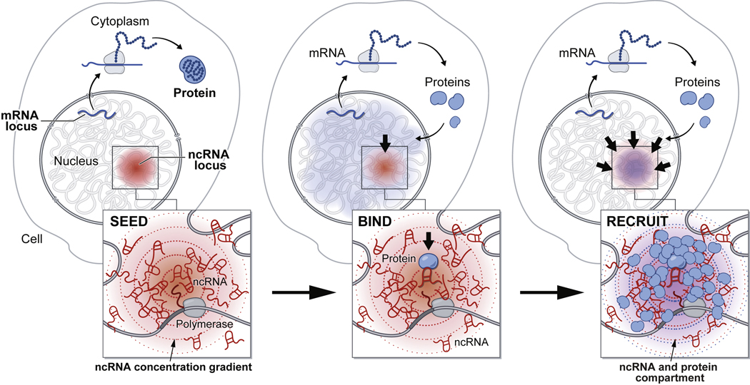
Once transcribed, mRNAs are exported to the cytoplasm while ncRNAs are retained in the nucleus. ncRNA transcription creates a transcript concentration gradient, highest near its transcriptional locus (SEED, left panel). Because ncRNAs can bind with high affinity to diffusible RNAs and proteins immediately upon transcription (BIND, middle panel), they can concentrate other RNAs and proteins in a spatial compartment (RECRUIT, right panel). In this way, ncRNAs can drive the organization of nuclear compartments. See also Figure S7.

More generally, we showed that hundreds of nuclear ncRNAs are preferentially localized within precise territories in the nucleus, suggesting that RNA may represent a widespread class of molecules that act as seeds to drive spatial organization of diffusible molecules. This mechanism utilizes a unique role for RNA in the nucleus (relative to DNA or proteins): the process of transcription produces many copies of an RNA, which accumulate at high concentrations in proximity to their transcriptional locus. In contrast, proteins are translated in the cytoplasm and therefore lack positional information in the nucleus, and DNA is present at a single copy and therefore cannot achieve high local concentrations.

Central to this mechanism is the fact that ncRNAs can form high affinity interactions immediately following transcription and thus can recruit proteins and RNAs. In contrast, mRNAs require translation and therefore generally do not form stable interactions with regulatory molecules in the nucleus. Our results suggest that any RNA that functions independently of its translated product could act in this way. For example, we find that histone pre-mRNAs can seed organization of nuclear compartments even though their processed RNAs are also translated into protein products. Other nascent pre-mRNAs may also have protein-independent functions and form high-affinity interactions within the nucleus that are important for spatial organization. This seeding role for RNA might also contribute to the formation of other recently described nuclear compartments such as transcriptional condensates, which inherently produce high levels of RNAs, including enhancer-associated RNAs and pre-mRNAs. Nonetheless, not all ncRNAs – or even all nuclear ncRNAs – act to form compartments around their loci since nuclear ncRNAs can also localize within other regions in the nucleus (e.g. Malat1, scaRNAs, snoRNAs, and snRNAs). Future work will be needed to understand why some specific nuclear RNAs are locally constrained while others diffuse throughout the nucleus.

Taken together, these results provide a global picture of how spatial enrichment of ncRNAs in the nucleus can seed formation of compartments that are required for a wide range of essential nuclear functions, including RNA processing, heterochromatin organization, and gene regulation (Figure S7). While we focused our analysis on ncRNAs in this work, we note that RD-SPRITE can also be applied to measure how gene expression relates to genome organization because it can detect the arrangement of nascent pre-mRNAs relative other RNAs (e.g. enhancer RNAs, pre-mRNAs) and 3D DNA structure. Beyond the nucleus, we anticipate that RD-SPRITE will also provide a powerful method to study the molecular organization, function, and mechanisms of RNA compartments and granules throughout the cell.

LIMITATIONS OF THE STUDY

We note several technical limitations of the RD-SPRITE method. It requires crosslinking, which may lead to biases in the types of interactions that are detected. Because this approach takes a snapshot in time, it cannot measure dynamic events. While we showed several examples of RNAs that are required for recruiting diffusible molecules into spatial compartments and identified hundreds more that localized in high concentration territories and therefore may act in this way, this mechanism may not hold true for every RNA. Future work is needed to explore the functional and mechanistic roles of individual ncRNAs.

STAR METHODS

RESOURCE AVAILABILITY

Lead Contact

Further information and requests for resources and reagents should be directed to and will be fulfilled by the Lead Contact, Mitchell Guttman (mguttman@caltech.edu).

Materials Availability

This study did not generate new unique reagents.

Data and Code Availability

• SPRITE datasets generated during this study have been deposited on GEO and are publicly available as of the date of publication at https://www.ncbi.nlm.nih.gov/geo/query/acc.cgi?acc=GSE151515. Accession numbers are listed in the key resources table.

• The original code for the SPRITE analysis pipeline used in this study is available on Github at https://github.com/GuttmanLab/sprite2.0-pipeline and https://github.com/GuttmanLab/sprite-pipeline. DOIs are listed in the key resources table.

• Any additional information required to reanalyze the data reported in this paper is available from the lead contact upon request.

EXPERIMENTAL MODEL AND SUBJECT DETAILS

Cell line generation, cell culture, and drug treatments

Cell lines used in this study.

We used the following cell lines in this study: (i) Female ES cells (pSM44 ES cell line) derived from a 129 × castaneous F1 mouse cross. These cells express Xist from the endogenous locus under control of a tetracycline-inducible promoter. The dox-inducible Xist gene is present on the 129 allele, enabling allele-specific analysis of Xist induction and X chromosome silencing. (ii) Female F1–21 mouse ES cells, where we replaced the endogenous Kcnq1ot1 promoter with a tetracycline-inducible promoter (Kcnq1ot1-inducible ES cell line). In the absence of Doxycycline, these cells do not express Kcnq1ot1; in the presence of Doxycycline, these cells express Kcnq1ot1. (iii) Female ES cells containing dCas9 fused to 4-copies of the SID transcriptional repression domain integrated into a single locus in the genome (dCas9–4XSID). (iv) pSM33 male ES cells (gift from K. Plath). These cells express Xist from the endogenous locus under control of a tetracycline-inducible promoter. (v) TX1072, a female mouse embryonic stem cell line (gift from E. Heard (Schulz et al., 2014)). These cells express Xist from the endogenous locus under control of a tetracycline-inducible promoter. (vi) HEK293T, a female human embryonic kidney cell line (ATCC Cat# CRL-3216, RRID:CVCL_0063).

Cell culture conditions.

All mouse ES cell lines were grown at 37°C under 7% CO₂ on plates coated with 0.2% gelatin (Sigma, G1393–100ML) and 1.75 μg/mL laminin (Life Technologies Corporation, #23017015) in serum-free 2i/LIF media composed as follows: 1:1 mix of DMEM/F-12 (Gibco) and Neurobasal (Gibco) supplemented with 1x N2 (Gibco), 0.5x B-27 (Gibco 17504–044), 2 mg/mL bovine insulin (Sigma), 1.37 μg/mL progesterone (Sigma), 5 mg/mL BSA Fraction V (Gibco), 0.1 mM 2-mercaptoethanol (Sigma), 5 ng/mL murine LIF (GlobalStem), 0.125 μM PD0325901 (SelleckChem) and 0.375 μM CHIR99021 (SelleckChem). 2i inhibitors were added fresh with each medium change, and cells were grown. Fresh medium was replaced every 24–48 hours depending on culture density, and passaged every 72 hours using 0.025% Trypsin (Life Technologies) supplemented with 1mM EDTA and chicken serum (1/100 diluted; Sigma), rinsing dissociated cells from the plates with DMEM/F12 containing 0.038% BSA Fraction V.

TX1072 mouse ES cells were grown on gelatin-coated flasks in serum-containing ES cell medium (high glucose DMEM (Sigma), 15% FBS (Gibco), 2 mM L-glutamine (Gibco), 1 mM sodium pyruvate (Gibco), 0.1 mM MEM non-essential amino acids (Gibco), 0.1 mM β-mercaptoethanol, 1000 U/mL leukemia inhibitory factor (LIF, Chemicon), and 2i (3 μM Gsk3 inhibitor CT-99021, 1 μM MEK inhibitor PD0325901). Cell culture media was changed daily.

HEK293T cells were cultured in complete media consisting of DMEM (GIBCO, Life Technologies) supplemented with 10% FBS (Seradigm Premium Grade HI FBS, VWR), 1X penicillin-streptomycin (GIBCO, Life Technologies), 1X MEM non-essential amino acids (GIBCO, Life Technologies), 1 mM sodium pyruvate (GIBCO, Life Technologies) and maintained at 37°C under 5% CO₂. For maintenance, 800,000 cells were seeded into 10 mL of complete media every 3–4 days in 10 cm dishes. HEK293T cells were used for human-mouse mixing experiments to assess noise during the SPRITE procedure as well as for imaging Coilin foci.

METHOD DETAILS

Doxycycline Inducible Xist Cell Line Development.

Female ES cells (F1 2–1 line, provided by K. Plath) were CRISPR-targeted (nicking gRNA pairs TGGGCGGGAGTCTTCTGGGCAGG and GGATTCTCCCAGGCCCAGGGCGG) to integrate the Tet transactivator (M2rtTA) into the Rosa26 locus using R26P-M2rtTA, a gift from Rudolf Jaenisch (Addgene plasmid #47381). This line was subsequently CRISPR-targeted (nicking gRNA pairs GCTCGTTTCCCGTGGATGTG and GCACGCCTTTAACTGATCCG) to replace the endogenous Xist promoter with tetracycline response elements (TRE) and a minimal CMV promoter as previously described (Engreitz et al., 2013). The promoter replacement insertion was verified by PCR amplification of the insertion locus and Sanger sequencing of the amplicon. SNPs within the amplicon allowed for allele identification of the insertion, confirming that the 129 allele was targeted and induced Xist expression. We routinely confirmed the presence of two X chromosomes within these cells by checking the presence of X-linked SNPs on the 129 and castaneous alleles.

3D-SIM SHARP-Halo cell culture conditions.

pSM33 cells were seeded in 4-well imaging chambers (ibidi) equipped with a high precision glass bottom and plasmids were transfected with lipofectamine 3000 24 hours prior to imaging according to the manufacturer’s instructions. Addition of doxycycline 8hrs prior to imaging was performed to transiently induce full-length (FL) SHARP and ΔRRM-SHARP SHARP (also known as Spen) expression from the Sp22 clone as previously described (Markaki et al., 2020). The ΔRRM clone (SHARPΔ1–591) was generated using PIPE mutagenesis using the Sp22 Full Length entry clone as template. It was recombined with appropriate destination vectors using Gateway LR recombination. 1μM JF646 Halo ligand was introduced to the media for 30 min, washed-off twice with PBS and exchanged with fresh media which were incubated for another 15 min. Live-cell 3D-SIM imaging was performed at 37C and 5% CO₂ in media without phenol red.

Doxycycline Inducible Kcnq1ot1 cell line development.

The endogenous promoter of Kcnq1ot1 was CRISPR-targeted (nicking gRNA pairs ACAGATGCTGAATAATGACT and CACGTCACCAAGGTCTTGGT or GCAGCCACGACACTGTTGAT and GTCACCAAGGTCTTGGTAGG) to insert a TRE and minimal CMV promoter into the same cell line with integrated Tet transactivator (M2rtTA) used to generate Dox-inducible Xist (see above). Clones were screened for ablation of endogenous Kcnq1ot1 expression and upregulation of expression upon administration of doxycycline (Supplemental Figure 6E,H).

CRISPRi: dCas9–4XSID cell line generation.

A catalytically dead Cas9 (dCas9) fused to 4 copies of the SID repressive domain (4XSID) expressed from an Ef1α promoter was integrated into a single copy locus in the genome (mm10 - chr6:86,565,487–86,565,506; gRNA sequence AATCTTAGTACTACTGCTGC) using CRISPR targeting (cells hereby referred to as dCas9–4XSID).

Doxycycline induction.

Xist and Kcnq1ot1 expression were induced in their respective cell lines by treating cells with 2 μg/mL doxycycline (Sigma D9891). Xist was induced for 24 hours prior to crosslinking and analysis. Kcnq1ot1 was induced for 12–16hrs prior to RNA harvesting for qRT-PCR or induced for 24hrs prior to cell crosslinking with 1% formaldehyde for ChIP-seq.

Trichostatin (TSA) treatment.

For HDAC inhibitor experiments, cells were treated with either DMSO (control) or 5μM TSA (Sigma T8552–1MG) in fresh 2i media or 2i media containing 2μg/ml doxycycline for induction of Kcnq1ot1 expression.

Flavopiridol (FVP) Treatment.

FVP transcriptional inhibition was performed by culturing cells in FVP (Sigma F3055–1MG) or DMSO at 1 μM final concentration in 2i media for 1 hour.

Actinomycin D (ActD) Treatment.

ActD transcriptional inhibition was performed by culturing cells in 25 μg/mL ActD (Sigma A9415, 25 μL of 1 mg/mL stock added per 1 mL culture medium) or DMSO for 4 hours before cells were processed for RNA-FISH, IF or SPRITE. The concentrations for imaging and for SPRITE were the same and the same stocks were used for all experiments.

Antibodies

Antibodies.

Primary antibodies used in the study: anti-Nucleolin (Abcam Cat# ab22758, RRID:AB_776878, 1:500); anti-NPAT (Abcam Cat# ab70595, RRID:AB_1269585, 1:100); anti-SMN (BD Biosciences Cat# 610646, RRID:AB_397973, 1:100); anti-HP1ß (Active Motif Cat# 39979, RRID:AB_2793416, 1:200); anti-Coilin (Abcam Cat # ab210785; Santa Cruz Biotechnology Cat# sc-55594, RRID:AB_1121780; Santa Cruz Biotechnology Cat# sc-56298, RRID:AB_1121778; 1:100); anti-Sharp (Bethyl Cat# A301–119A, RRID:AB_873132, 1:200); anti-Histone H3K27ac (Active Motif Cat# 39134, RRID:AB_2722569); anti-NPM1 (Abcam Cat# ab10530, RRID:AB_297271; 1:200); anti-Fibrillarin (Abcam Cat# ab5821, RRID:AB_2105785; 1:200); anti-LaminB1 (Abcam Cat# ab16048, RRID:AB_10107828; 1:1000); For imaging studies, all antibodies were diluted in blocking solution.

RNA & DNA-SPRITE

RD-SPRITE is an adaptation of our initial SPRITE protocol (Quinodoz et al., 2018) with significant improvements to the RNA molecular biology steps that enable generation of higher complexity RNA libraries.

RD-SPRITE improves efficiency of RNA tagging.

Although our previous version of SPRITE could map both RNA and DNA, it was limited primarily to detecting highly abundant RNA species (e.g. 45S pre-rRNA). In RD-SPRITE, we have improved detection of lower abundance RNAs by increasing yield through the following adaptations. (i) We increased the RNA ligation efficiency by utilizing a higher concentration of RPM, corresponding to ~2000 molar excess during RNA ligation. (ii) Adaptor dimers that are formed through residual purification on our magnetic beads lead to reduced efficiency because they preferentially amplify and preclude amplification of tagged RNAs. To reduce the number of adaptor dimers in library generation, we introduced an exonuclease digestion of excess reverse transcription (RT) primer that dramatically reduces the presence of the RT primer. (iii) Reverse transcription is used to add the barcode to the RNA molecule, yet when RT is performed on crosslinked material it will not efficiently reverse transcribe the entire RNA (because crosslinked proteins will act to sterically preclude RT). To address this, we performed a short RT in crosslinked samples followed by a second RT reaction after reverse crosslinking to copy the remainder of the RNA fragment. (iv) Because cDNA is single stranded, we need to ligate a second adaptor to enable PCR amplification. The efficiency of this reaction is critical for ensuring that we detect each RNA molecule. We significantly improved cDNA ligation efficiency by introducing a modified “splint” ligation. Specifically, a double stranded “splint” adaptor containing the Read1 Illumina priming region and a random 6mer overhang is ligated to the 3’end of the cDNA at high efficiency by performing a double stranded DNA ligation. This process is more efficient than the single stranded DNA-DNA ligation previously utilized (Quinodoz et al., 2018). (v) Finally, we found that nucleic acid purification performed after reverse crosslinking leads to major loss of complexity because we lose a percentage of the unique molecules during each cleanup. In the initial RNA-DNA SPRITE protocol there were several column (or bead) purifications utilized to remove enzymes and enable the next enzymatic reaction. We reduced these cleanups by introducing biotin modifications into the DPM and RPM adaptors that enable binding to streptavidin beads and for all subsequent molecular biology steps to occur on the same beads. Together, these improvements enabled a dramatic improvement of our overall RNA recovery and enables generation of high complexity RNA/DNA structure maps.

The approach was performed as follows:

Crosslinking, lysis, sonication, and chromatin digestion.

pSM44 mES cells were lifted using trypsinization and were crosslinked in suspension at room temperature with 2 mM disuccinimidyl glutarate (DSG) for 45 minutes followed by 3% Formaldehyde for 10 minutes to preserve RNA and DNA interactions in situ. After crosslinking, the formaldehyde crosslinker was quenched with addition of 2.5M Glycine for final concentration of 0.5M for 5 minutes, cells were spun down, and resuspended in 1x PBS + 0.5% RNAse Free BSA (AmericanBio AB01243–00050) over three washes, 1x PBS + 0.5% RNAse Free BSA was removed, and flash frozen at −80C for storage. We found that RNAse Free BSA is critical to avoid RNA degradation. RNase Inhibitor (1:40, NEB Murine RNAse Inhibitor or Thermofisher Ribolock) was also added to all lysis buffers and subsequent steps to avoid RNA degradation. After lysis, cells were sonicated at 4–5W of power for 1 minute (pulses 0.7 second on, 3.3 seconds off) using the Branson Sonicator and chromatin was fragmented using DNAse digestion to obtain DNA of approximately ~150bp-1kb in length.

Estimating molarity.

After DNase digestion, crosslinks were reversed on approximately 10 μL of lysate in 82 μL of 1X Proteinase K Buffer (20 mM Tris pH 7.5, 100 mM NaCl, 10 mM EDTA, 10 mM EGTA, 0.5% Triton-X, 0.2% SDS) with 8 μL Proteinase K (NEB) at 65°C for 1 hour. RNA and DNA were purified using Zymo RNA Clean and Concentrate columns per the manufacturer’s specifications (>17nt protocol) with minor adaptations, such as binding twice to the column with 2X volume RNA Binding Buffer combined with by 1X volume 100% EtOH to improve yield. Molarities of the RNA and DNA were calculated by measuring the RNA and DNA concentration using the Qubit Fluorometer (HS RNA kit, HS dsDNA kit) and the average RNA and DNA sizes were estimated using the RNA High Sensitivity Tapestation and Agilent Bioanalyzer (High Sensitivity DNA kit).

NHS bead coupling.

We used the RNA and DNA molarity estimated in the lysate to calculate the total number of RNA and DNA molecules per microliter of crosslinked lysate. We coupled the lysate to ~10mL of NHS-activated magnetic beads (Pierce) in 1x PBS + 0.1% SDS combined with 1:40 dilution of NEB Murine RNase Inhibitor overnight at 4°C. We coupled at a ratio of 0.25–0.5 molecules per bead to reduce the probability of simultaneously coupling multiple independent complexes to the same bead, which would lead to their association during the split-pool barcoding process. Because multiple molecules of DNA and RNA can be crosslinked in a single complex, this estimate is a more conservative estimate of the number of molecules to avoid collisions on individual beads. After NHS coupling overnight, the supernatant was removed and 0.5M Tris pH 7.5 was added for 1 hour at 4°C to quench coupling. Beads were subsequently washed post coupling three times with 1mL of Modified RLT buffer and three times with 1mL of SPRITE Wash buffer.

Because the crosslinked complexes are immobilized on NHS magnetic beads, we can perform several enzymatic steps by adding buffers and enzymes directly to the beads and performing rapid buffer exchange between each step on a magnet. All enzymatic steps were performed with shaking at 1200–1600 rpm (Eppendorf Thermomixer) to avoid bead settling and aggregation. All enzymatic steps were inactivated either by adding 1 mL of SPRITE Wash buffer (20mM Tris-HCl pH 7.5, 50mM NaCl, 0.2% Triton-X, 0.2% NP-40, 0.2% Sodium deoxycholate) supplemented with 50 mM EDTA and 50 mM EGTA to the NHS beads or Modified RLT buffer (1x Buffer RLT supplied by Qiagen, 10mM Tris-HCl pH 7.5, 1mM EDTA, 1mM EGTA, 0.2% N-Lauroylsarcosine, 0.1% Triton-X, 0.1% NP-40).

DNA End Repair and dA-tailing.

We then repair the DNA ends to enable ligation of tags to each molecule. Specifically, we blunt end and phosphorylate the 5’ ends of double-stranded DNA using two enzymes. First, the NEBNext End Repair Enzyme cocktail (E6050L; containing T4 DNA Polymerase and T4 PNK) and 1x NEBNext End Repair Reaction Buffer is added to beads and incubated at 20°C for 1 hour, and inactivated and buffer exchanged as specified above. DNA was then dA-tailed using the Klenow fragment (5’−3’ exo-, NEBNext dA-tailing Module; E6053L) at 37°C for 1 hour, and inactivated and buffer exchanged as specified above. Note, we do not use the NEBNext Ultra End Repair/dA-tailing module as the temperatures in the protocol are not compatible with SPRITE as the higher temperature will reverse crosslinks. To prevent degradation of RNA, each enzymatic step is performed with the addition of 1:40 NEB Murine RNAse Inhibitor or Thermofisher Ribolock.

Ligation of the DNA Phosphate Modified (“DPM”) Tag.

After end repair and dA-tailing of DNA, we performed a pooled ligation with “DNA Phosphate Modified” (DPM) tag that contains certain modifications that we found to be critical for the success of RD-SPRITE. Specifically, (i) we incorporate a phosphothiorate modification into the DPM adaptor to prevent its enzymatic digestion by Exo1 in subsequent RNA steps and (ii) we integrated an internal biotin modification to facilitate an on-bead library preparation post reverse-crosslinking. The DPM adaptor also contains a 5’phosphorylated sticky end overhang to ligate tags during split-pool barcoding. DPM Ligation was performed using 11 μL of μM DPM adaptor in a 250 μL reaction using Instant Sticky End Mastermix (NEB) at 20°C for 30 minutes with shaking. All ligations were supplemented with 1:40 RNAse inhibitor (ThermoFisher Ribolock or NEB Murine RNase Inhibitor) to prevent RNA degradation. Because T4 DNA Ligase only ligates to double-stranded DNA, the unique DPM sequence enables accurate identification of DNA molecules after sequencing.

Ligation of the RNA Phosphate Modified (“RPM”) Tag.

To map RNA and DNA interactions simultaneously, we ligated an RNA adaptor to RNA that contains the same 7nt 5’phosphorylated sticky end overhang as the DPM adaptor to ligate tags to both RNA and DNA during split-pool barcoding. To do this, we first modify the 3’end of RNA to ensure that they all have a 3’OH that is compatible for ligation. Specifically, RNA overhangs are repaired with T4 Polynucleoide Kinase (NEB) with no ATP at 37°C for 20 min. RNA is subsequently ligated with a “RNA Phosphate Modified” (RPM) adaptor using High Concentration T4 RNA Ligase I (Shishkin et al., 2015). Briefly, beads were resuspended in a solution consisting of 30 μL 100% DMSO, 154 μL H₂O, and 20 μL of 20 μM RPM adaptor, heated at 65°C for 2 minutes to denature secondary structure of RNA and the RPM adaptor, then immediately put on ice. An RNA ligation master mix was added on top of this mixture consisting of: 40 μL 10x NEB T4 RNA Ligase Buffer, 4 μL 100mM ATP (NEB), 120 μL 50% PEG 8000 (NEB), 20 μL Ultra Pure H₂O, 6 μL Ribolock RNAse Inhibitor, 7 μL NEB T4 RNA Ligase, High Concentration (M0437M) for 24°C for with shaking 1 hour 15 minutes. Because T4 RNA Ligase 1 only ligates to single-stranded RNA, the unique RPM sequence enables accurate identification of RNA and DNA molecules after sequencing. After RPM ligation, RNA was converted to cDNA using Superscript III at 42°C for 1 hour using the “RPM bottom” RT primer that contains an internal biotin to facilitate on-bead library construction (as above) and a 5’end sticky end to ligate tags during SPRITE. Excess primer is digested with Exonuclease 1 at 42°C for 10–15 min. All ligations were supplemented with 1:40 RNAse inhibitor (ThermoFisher Ribolock or NEB Murine RNase Inhibitor) to prevent RNA degradation.

Split-and-pool barcoding to identify RNA and DNA interactions.

The beads were then repeatedly split-and-pool ligated over four rounds with a set of “Odd,” “Even” and “Terminal” tags (see SPRITE Tag Design (Quinodoz et al., 2018)). Both DPM and RPM contain the same 7 nucleotide sticky end that will ligate to all subsequent split-pool barcoding rounds. All split-pool ligation steps were performed for 45min to 1 hour at 20°C. Specifically, each well contained the following: 2.4 μL well-specific 0.45 μM SPRITE tag (IDT), 6.4 μL custom SPRITE ligation master mix, 5.6 μL SPRITE wash buffer (described above), and 5.6 μL Ultra-Pure H₂O. For all SPRITE ligations, we make a custom SPRITE ligation master mix (3.125x concentrated) combining 1600 μL of 2x Instant Sticky End Mastermix (NEB; M0370), 600 μL of 1,2-Propanediol (Sigma-Aldrich; 398039), and 1000 μL of 5x NEBNext Quick Ligation Reaction Buffer (NEB; B6058S). All ligations were supplemented with 1:40 RNAse inhibitor (ThermoFisher Ribolock or NEB Murine RNase Inhibitor) to prevent RNA degradation.

Reverse crosslinking.

After multiple rounds of SPRITE split-and-pool barcoding, the tagged RNA and DNA molecules are eluted from NHS beads by reverse crosslinking overnight (~12–13 hours) at 50°C in NLS Elution Buffer (20mM Tris-HCl pH 7.5, 10mM EDTA, 2% N-Lauroylsarcosine, 50mM NaCl) with added 5M NaCl to 288 mM NaCl Final combined with 5 μL Proteinase K (NEB).

Post reverse-crosslinking library preparation.

AEBSF (Gold Biotechnology CAS#30827–99-7) is added to the Proteinase K (NEB Proteinase K #P8107S; ProK) reactions to inactive the ProK prior to coupling to streptavidin beads. Biotinylated barcoded RNA and DNA are bound to Dynabeads™ MyOne™ Streptavidin C1 beads (ThermoFisher #65001). To improve recovery, the supernatant is bound again to 20μL of streptavidin beads and combined with the first capture. Beads are washed in 1X PBS + RNase inhibitor and then resuspended in 1x First Strand buffer to prevent any melting of the RNA:cDNA hybrid. Beads were pre-incubated at 40C for 2 min to prevent any sticky barcodes from annealing and extending prior to adding the RT enzyme. A second reverse transcription is performed by adding Superscript III (Invitrogen #18080051) (without RT primer) to extend the cDNA through the areas which were previously crosslinked. The second RT ensures that cDNA recovery is maximal, particularly if RT terminated at a crosslinked site prior to reverse crosslinking. After generating cDNA, the RNA is degraded by addition of RNaseH (NEB # M0297) and RNase cocktail (Invitrogen #AM2288), and the 3’end of the resulting cDNA is ligated to attach an dsDNA oligo containing library amplification sequences for subsequent amplification.

Previously, we performed cDNA (ssDNA) to ssDNA primer ligation which relies on the two single stranded sequences coming together for conversion to a product that can then be amplified for library preparation. To improve the efficiency of cDNA molecules ligated with the Read1 Illumina priming sequence, we perform a “splint” ligation, which involves a chimeric ssDNA-dsDNA adaptor that contains a random 6mer that anneals to the 3’ end of the cDNA and brings the 5’ phosphorylated end of the cDNA adapter directly together with the cDNA via annealing. This ligation is performed with 1x Instant Sticky End Master Mix (NEB #M0370) at 20°C for 1 hour. This greatly improves the cDNA tagging and overall RNA yield.

Libraries were amplified using 2x Q5 Hot-Start Mastermix (NEB #M0494) with primers that add the indexed full Illumina adaptor sequences. After amplification, the libraries are cleaned up using 0.8X SPRI (AMPure XP) and then gel cut using the Zymo Gel Extraction Kit selecting for sizes between 280 bp - 1.3 kb. A calculator for estimating the number of reads required to reach a saturated signal depth for each library are provided in Supplemental Table 4.

Sequencing.

Sequencing was performed on an Illumina NovaSeq S4 paired-end 150×150 cycle run. For the mES RNA-DNA RD-SPRITE data in this experiment, 144 different SPRITE libraries were generated from four technical replicate SPRITE experiments and were sequenced. The four experiments were generated using the same batch of crosslinked lysate processed on different days to NHS beads. Each SPRITE library corresponds to a distinct aliquot during the Proteinase K reverse crosslinking step which is separately amplified with a different barcoded primer, providing an additional round of SPRITE barcoding.

Primers Used for RPM, DPM, and Splint Ligation (IDT):

1. RPM top: /5Phos/rArUrCrArGrCrACTTAGCG TCAG/3SpC3/

2. RPM bottom (internal biotin): /5Phos/TGACTTGC/iBiodT/GACGCTAAGTGCTGAT

3. DPM Phosphorothioate top: /5Phos/AAGACCACCAGATCGGAAGAGCGTCGTG*T* A*G*G* /32MOErG/ *Denotes Phosphorothioate bonds

4. DPM bottom (internal biotin): /5Phos/TGACTTGTCATGTCT/iBioT/CCGATCTGGTGGTCTTT

5. 2Puni splint top: TACACGACGCTCTTCCGATCT NNNNNN/3SpC3/

6. 2Puni splint bottom: /5Phos/AGA TCG GAA GAG CGT CGT GTA/3SpC3/

Annealing of adaptors.

A double-stranded DPM oligo and 2P universal “splint” oligo were generated by annealing the complementary top and bottom strands at equimolar concentrations. Specifically, all dsDNA SPRITE oligos were annealed in 1x Annealing Buffer (0.2 M LiCl₂, 10 mM Tris-HCl pH 7.5) by heating to 95°C and then slowly cooling to room temperature (−1°C every 10 sec) using a thermocycler.

Assessing molecule to bead ratio.

We ensured that SPRITE clusters represent bona fide interactions that occur within a cell by mixing human and mouse cells and ensuring that virtually all SPRITE clusters (~99%) represent molecules exclusively from a single species. Specifically, we separately crosslinked HEK293T cells performed a human-mouse mixing RD-SPRITE experiment and identified conditions with low interspecies mixing (molecules = RNA+DNA instead of DNA). Specifically, for SPRITE clusters containing 2–1000 reads, the percent of interspecies contacts is: 2 beads:molecule = 0.9% interspecies contacts, 4 beads:molecule = 1.1% interspecies contacts, 8 beads:molecule = 1.1% interspecies contacts. We used the 2 beads:molecule and 4 beads:molecule ratio for the RD-SPRITE data sets generated in this paper.

RD-SPRITE technical replicates.

One of the RD-SPRITE replicate libraries was generated with a DPM lacking the phosphorothioate bond and 2’-O-methoxy-ethyl bases on the 3’end of the top adaptor. We found that this resulted in a lower number of DNA reads because the exonuclease step can degrade the single-stranded portion of the DPM oligo. As a result, this library has lower DNA-DNA and DNA-RNA pairs, but has more RNA-RNA contacts overall. This experiment was analyzed to generate higher-resolution RNA-RNA contact matrices, including contacts of lower abundance RNAs. The three other RD-SPRITE replicate libraries were generated with the same batch crosslinked lysate but were ligated with a DPM adaptor containing these modifications to prevent DNA degradation.

RD-SPRITE processing pipeline

Adapter trimming.

Adapters were trimmed from raw paired-end fastq files using Trim Galore! v0.6.2 (https://www.bioinformatics.babraham.ac.uk/projects/trim_galore/) and assessed with Fastqc v0.11.9. Subsequently, the DPM (GATCGGAAGAG) and RPM (ATCAGCACTTA) sequences are trimmed using Cutadapt v2.5(Martin, 2011) from the 5’ end of Read 1 along with the 3’ end DPM sequences that result from short reads being read through into the barcode (GGTGGTCTTT, GCCTCTTGTT, CCAGGTATTT, TAAGAGAGTT, TTCTCCTCTT, ACCCTCGATT). The additional trimming helps improve read mapping in the end-to-end alignment mode. The SPRITE barcodes of trimmed reads are identified with Barcode ID v1.2.0 (https://github.com/GuttmanLab/sprite2.0-pipeline) and the ligation efficiency is assessed. Reads with an RPM or a DPM barcode are split into two separate files, to process RNA and DNA reads individually downstream, respectively.

Ligation Efficiency Quality Control.

We assessed the reproducibility and quality of an RD-SPRITE experiment by calculating the ligation efficiency, defined as the proportion of sequencing reads containing only 1, 2, 3… through n barcodes (where n is the number of rounds of split-pool barcoding). Across technical replicates, biological replicates, and multiple sequencing libraries, we have found highly similar ligation efficiencies, with ~60% or more of reads containing all 5 barcoding tags (see Supplemental Table 3).

Processing RNA reads.

RNA reads were aligned to GRCm38.p6 with the Ensembl GRCm38 v95 gene model annotation using Hisat2 v2.1.0 (Kim et al., 2015) with a high penalty for soft-clipping --sp 1000,1000. Unmapped and reads with a low MapQ score (samtools view -bq 20) were filtered out for downstream realignment. (see Supplemental Table 2 for alignment statistics). Mapped reads were annotated for gene exons and introns with the featureCounts tool from the subread package v1.6.4 using Ensembl GRCm38 v95 gene model annotation and the Repeat and Transposable element annotation from the Hammel lab (Jin et al., 2015). Filtered reads were subsequently realigned to our custom collection of repeat sequences using Bowtie v2.3.5 (Langmead and Salzberg, 2012), only keeping mapped and primary alignment reads.

Processing DNA reads.

DNA reads were aligned to GRCm38.p6 using Bowtie2 v2.3.5 (see Supplemental Table 2 for alignment statistics), filtering out unmapped and reads with a low MapQ score (samtools view -bq 20). Data generated in F1 hybrid cells (pSM44: 129 × castaneous) were assigned the allele of origin using SNPsplit v0.3.4 (Krueger and Andrews, 2016). RepeatMasker (Smit et al., 2015) defined regions with milliDev ≤ 140 along with blacklisted v2 regions were filtered out using Bedtools v2.29.0 (Quinlan and Hall, 2010).

SPRITE cluster file generation.

RNA and DNA reads were merged, and a cluster file was generated for all downstream analysis. MultiQC v1.6 (Ewels et al., 2016) was used to aggregate all reports.

Masked bins.

In addition to known repeat containing bins, we manually masked the following bins (mm10 genomic regions: chr2:79490000–79500000, chr11:3119270–3192250, chr15:99734977–99736026, chr3:5173978–5175025, chr13:58176952–58178051) because we observed a major overrepresentation of reads in the input samples.

Microscopy imaging

3D-Structured Illumination Microscopy (3D-SIM):

3D-SIM super-resolution imaging was performed on a DeltaVision OMX-SR system (Cytiva, Marlborough, MA, USA) equipped with a 60x/1.42 NA Plan Apo oil immersion objective (Olympus, Tokyo, Japan), sCMOS cameras (PCO, Kelheim, Germany) and 642 nm diode laser. Image stacks were acquired with z-steps of 125 nm and with 15 raw images per plane. The raw data were computationally reconstructed with the soft-WoRx 7.0.0 software package (Cytiva, Marlborough, MA, USA) using a wiener filter set to 0.002 and channel-specifically measured optical transfer functions (OTFs) using an immersion oil with a 1.518 refractive index (RI). 32-bit raw datasets were imported to ImageJ and converted to 16-bit stacks.

Immunofluorescence (IF).

Cells were grown on coverslips and rinsed with 1x PBS, fixed in 4% paraformaldehyde in PBS for 15 minutes at room temperature, rinsed in 1x PBS, and permeabilized with 0.5% Triton X-100 in PBS for 10 minutes at room temperature. Cells were either stored at −20°C in 70% ethanol or used directly for immunostaining and incubated in blocking solution (0.2% BSA in PBS) for at least 1 hour. If stored in 70% ethanol, cells were re-hydrated prior to staining by washing 3 times in 1xPBS and incubated in blocking solution (0.2% BSA in PBS) for at least 1 hour. Primary antibodies were diluted in blocking solution and added to coverslips for 3–5 hours at room temperature incubation. Cells were washed three times with 0.01% Triton X-100 in PBS for 5 minutes each and then incubated in blocking solution containing corresponding secondary antibodies labeled with Alexa fluorophores (Invitrogen) for 1 hour at room temperature. Next, cells were washed 3 times in 1xPBS for 5 minutes at room temperature and mounting was done in ProLong Gold with DAPI (Invitrogen, P36935). Images were collected on a LSM800 or LSM980 confocal microscope (Zeiss) with a 63× oil objective. Z sections were taken every 0.3 μm. Image visualization and analysis was performed with Icy software (http://icy.bioimageanalysis.org/) and ImageJ software (https://imagej.nih.gov/).

Immunofluorescence (IF) for ActD experiments.

Cells were cultured in DMSO or ActD (Sigma A9415, 25μL of 1mg/mL stock added per 1ml culture medium) for 4 hours, then fixed and processed for IF using the anti-NPAT antibody, as described earlier. Images were acquired using the Zeiss LSM980 microscope with 63x oil objective and 16 Z-sections were taken with 0.3 μm increments. To count the number of NPAT spots, we generated the maximal projections, defined a binary mask by thresholding based on background intensity levels, and manually counted the number of spots for each nucleus.

RNA Fluorescence in situ Hybridization (RNA-FISH).

RNA-FISH performed in this study was based on the ViewRNA ISH (Thermo Fisher Scientific, QVC0001) protocol with minor modifications. Cells grown on coverslips were rinsed in 1xPBS, fixed in 4% paraformaldehyde in 1xPBS for 15 minutes at room temperature, permeabilized in 0.5% Triton-100 in the fixative for 10 minutes at room temperature, rinsed 3 times with 1xPBS and stored at −20°C in 70% ethanol until hybridization steps. All the following steps were performed according to manufacturer’s recommendations. Coverslips were mounted with ProLong Gold with DAPI (Invitrogen, P36935) and stored at 4°C until acquisition. For nuclear and nucleolar RNAs, cells were pre-extracted with 0.5% ice cold Triton-100 for 3 minutes to remove cytoplasmic background and fixed as described. All probes used in the study were custom made by Thermofisher (order numbers available upon request). To test their specificity, we either utilized RNAse treatment prior to RNA-FISH or two different probes targeting the same RNA. Images were acquired on Zeiss LSM800 or LSM980 confocal microscope with a 100x glycerol immersion objective lens and Z-sections were taken every 0.3 μm. Image visualization and analysis was performed with Icy software and ImageJ software.

RNA FISH for scaRNA and tRNAs were performed with a combined set of probes to increase the signal of lower abundance RNAs. Specifically, scaRNAs were visualized with two combined probes of scaRNA2 and scaRNA17. tRNAs were visualized using probes targeting tRNA-Arg-TCG-4–1, tRNA-Leu-AAG-3–1, tRNA-Ile-AAT-1–8, tRNA-Arg-TCT-5–1, tRNA-Leu-CAA-2–1, tRNA-Ile-TAT-2–1, tRNA-Tyr-GTA-1–1. tRNA sequences were obtained using the GtRNAdb GRCm38/mm10 predictions (Lowe Lab, UCSC)(Chan and Lowe, 2009, 2016).

RNA-FISH for FVP experiments.

To compare the relative stability of lncRNAs and pre-mRNAs, we obtained intron FISH probes for targets of comparable gene length to lncRNAs. This was done to ensure that any differences in RNA stability upon FVP treatment are not due to differences in the time it takes to transcribe each RNA. Specifically, we obtained probes for pre-mRNAs that are 57.87kb (Nup188), 73.7kb (Mbd5), 99.8kb (Abi1), 129.7kb (Ehmt1),131.8kb (Atrx), and 297.2kb (Gtdc1) in length. For lncRNAs, we obtained probes for RNAs of lengths 53.4kb (Tsix), 79.5kb (Dleu2), 93.1kb (Kcnq1ot1), and 340kb (Pvt1).

RNA-FISH combined with immunofluorescence of SHARP at Kcnq1ot1 loci.

Dox inducible Kcnq1ot1 mESC were cultured in dox for 24 hours and fixed for RNA-FISH against Kcnq1ot1 and Nap1l4 combined with immunofluorescence for SHARP. Images were acquired on a Zeiss LSM980 confocal microscope with 63x oil immersion objective lens using the Airyscan 2.0 detector. The number of z-slices and size of the image were determined based on Zeiss recommendations for optimal Airyscan 2.0 acquisition. All images were deconvoluted using ZEN Blue Software with the same settings and were analyzed using Imaris software. To visualize the locations of the two alleles, we used the spot detection module to identify 3D surfaces corresponding to either Nap1l4 or Kcnq1ot1 signals. Spots positive for Nap1l4 RNA but not Kcnq1ot1 are referred to as Kcnq1ot1- and spots positive for Kcnq1ot1 are referred to as Kcnq1ot1+ alleles in this manuscript. The same thresholds and size filters were used across all images and the determined 3D objects were of the same volumes. For quality control, we confirmed that the majority of cells only contained a single Kcnq1ot1 volume and filtered the few individual cells containing zero or two volumes. This ensured that we focus only on cells with monoallelic expression of Kcnq1ot1. We quantified fluorescence intensity in these 3D objects by taking the sum of intensity within those volumes across all channels and plotted the resulting values.

Combined RNA-FISH and IF.

For immunostaining combined with in situ RNA visualization, we used the ViewRNA Cell Plus (Thermo Fisher Scientific, 88–19000-99) kit per the manufacturer’s protocol with minor modifications. Immunostaining was performed as described above, but all incubations were performed in blocking buffer with addition of RNAse inhibitor and all the wash steps were performed in RNAse free 1x PBS with RNAse inhibitor. Blocking buffer, PBS, RNAse inhibitors are provided in a kit. After the last wash in 1x PBS, cells underwent post-fixation in 2% paraformaldehyde on 1x PBS for 10min at room temperature, were washed 3 times in 1x PBS, and then RNA-FISH protocol was followed as described above. Images were acquired on the Zeiss LSM800 or LSM980 confocal microscope with a 100x glycerol immersion objective lens and z-sections were taken every 0.3 μm. Image visualization and analysis was performed with Icy software and ImageJ software.

DNA-FISH.

DNA-FISH was performed as previously described (Bolzer et al., 2005) with modifications. Cells grown on coverslips were rinsed with 1x PBS, fixed in 4% paraformaldehyde in 1x PBS for 15 minutes at room temperature, permeabilized in 0.5% Triton-100 in the fixative for 10 minutes at room temperature, rinsed 3 times with 1x PBS and stored at −20°C in 70% ethanol until hybridization steps. Pre-hybridization cells were dehydrated in 100% ethanol and dried for 5 minutes at room temperature. 4 μL drop of hybridization mix with probes was spotted on a glass slide and dried coverslips were placed on the drop. Coverslips were sealed with rubber cement, slides were incubated for 5 minutes at 85°C, and then incubated overnight at 37°C in humid atmosphere. After hybridization and three washes with 2x SSC, 0.05% Triton-100 and 1mg/mL PVP in PBS at 50°C for 10 minutes, cells were rinsed in 1x PBS and mounted with ProLong Gold with DAPI (Invitrogen, P36935).

Hybridization buffer consisted of 50% formamide, 10% dextran sulphate, 2xSSC, 1 mg/mL polyvinyl pyrrolidone (PVP), 0.05% Triton X-100, 0.5 mg/mL BSA. 1 mM short oligonucleotides labeled with Cy5 ([CY5]ttttctcgccatattccaggtc) were used as probes against Major Satellites and full-length minor satellite repeat sequence was used as probes against Minor Satellites. Minor satellite sequence was firstly cloned to pGEM plasmid and then labeled by PCR reaction with self-made TAMRA dATPs for minor satellites. Labeled PCR product was purified with a QIAquick PCR Purification Kit (QIAGEN), and 50 ng was mixed with hybridization buffer. Images were acquired on Zeiss LSM800 or LSM980 confocal microscope with a 63x glycerol immersion objective lens and Z-sections were taken every 0.3 μm. Image visualization and analysis was performed with Icy software and ImageJ software.

Analysis of RNA-DNA contacts

Generating contact profiles.

To map the genome-wide localization profile of a specific RNA, we calculated the contact frequency between the RNA transcript and each region of the genome binned at various resolutions (1Mb, 100kb and 10kb). Raw contact frequencies were computed by counting the number of SPRITE clusters in which an RNA transcript and a genomic bin co-occur. We normalized these raw contacts by weighting each contact by a scaling factor based on the size of its corresponding SPRITE cluster. Specifically, we enumerate all pairwise contacts within a SPRITE cluster and weight each contact by 2/n, where n is the total number of reads within a cluster.

RNA and cluster sizes.

RNA-DNA contacts were computed for a range of SPRITE cluster sizes, such as 2–10, 11–100, and 101–1000, ≥1001 reads. We found that different RNAs tend to be most represented in different clusters sizes – likely reflecting the size of the nuclear compartment that they occupy. For example, 45S and snoRNAs are most represented in large clusters, while Malat1, snRNAs, and other ncRNAs tend to be represented in smaller SPRITE clusters. For analyses in this paper, we utilized clusters containing 2–1000 reads unless otherwise noted.

Visualizing contact profiles.

These methods produce a one-dimensional vector of DNA contact frequencies for each RNA transcript that we output in bedgraph format and visualize with IGV (Robinson et al., 2011). To compare DNA contact profiles between RNA transcripts, we calculated a Pearson correlation coefficient between the one-dimensional DNA contact vectors for all pairs of RNA transcripts.

Aggregate analysis of RNA-DNA contacts.

To map RNA-DNA localization across chromosomes with respect to centromeres and telomeres (e.g. Terc and satellite ncRNAs), we computed an average localization profile as a function of distance from the centromere of each chromosomes. To do this, we converted each 1Mb genomic bin into a percentile bin from 0 to 100 based on its relative position on its chromosome (from 5’ to 3’ ends). We then calculated the average contact frequency for a given RNA with each percentile bin across all chromosomes.

Allele specific analysis.

To map localization to different alleles, we identified all clusters containing a given RNA (as above) and quantified the number of DNA reads uniquely mapping to each allele using allele specific alignments. Allele specific RNA-DNA contact frequencies were normalized by overall genomic read coverage for each allele to account for differences in coverage for each allele.

Nucleolar hub RNA-DNA contacts.

We observe enrichment of pre-rRNAs and other nucleolar hub RNAs on chromosomes containing 45S ribosomal DNA (rDNA). Specifically, rDNA genes are contained on the centromere-proximal regions of chromosomes 12, 15, 16, 18, and 19 in mouse ES cells. We previously showed that regions on these chromosomes organize around nucleoli in the majority of cells imaged with DNA FISH combined with immunofluorescence for Nucleolin (Quinodoz et al., 2018). We also observed nucleolar hub RNAs enriched on other genomic regions corresponding to centromere-proximal DNA and transcriptionally inactive, gene poor regions. We previously showed that these genomic regions are organized proximal to the nucleolus using SPRITE and microscopy (Quinodoz et al., 2018).

Splicing RNA concentration relative to nuclear speckle distance.

We observed that snRNAs are enriched over genomic regions with high gene-density, which we have previously shown organize around the nuclear speckle (Quinodoz et al., 2018). To explore whether splicing RNA concentration is related to genomic DNA distance to nuclear speckles, we computed the RNA-DNA contact profile for U1 snRNA in 10 kb bins across the genome, weighted by cluster size. For the same 10 kb bins, we calculated the RNA expression levels (the number of clusters containing the pre-mRNA) and filtered for bins with RNA counts > 100. In our dataset, this filter selects for genomic regions with high gene expression levels regardless of speckle distance. We then generated a “distance to speckle” metric for each genomic bin using DNA-DNA SPRITE measurements. This “distance” is defined as the average inter-chromosomal contact frequency between a given bin and genomic bins corresponding to the “active” hub (i.e. “speckle” hub). A larger contact frequency value is considered “close to the speckle” while a smaller value is “far from the speckle”. We grouped the 10 kb bins into 5 groups based on the “distance to speckle” metric and focused our subsequent analysis on the “closest” and “farthest” groups. Closest regions contained a normalized speckle distance score between 0.4–0.5 and farthest contained a score from 0–0.1. We then compared the distribution of U1 density over genes close to or far from the nuclear speckle.

Analysis of RNA-RNA contacts

RNA-RNA contact matrices.

We computed the contact frequency between each RNA-RNA pair by counting the number of SPRITE clusters containing two different RNAs. To account for coverage differences in individual RNAs, we normalized this matrix using a matrix balancing normalization approach as previously described (Imakaev et al., 2012). Briefly, this approach works by ensuring the rows and columns of a symmetric matrix add up to 1. In this way, RNA abundance does not dominate the overall strength of the contact matrix. For multi-copy RNAs (e.g. repeat-encoded RNAs, ribosomal RNA, tRNAs), all reads mapping to a given RNA were collapsed. Specifically, multi-copy RNA reads mapping to either the mm10 genome annotated using repeat masker or a custom repeat genome consensus were collapsed.

RNA Hubs.

Groups of pairwise interacting RNAs were first identified using hierarchical clustering of the pairwise RNA-RNA contact matrix. Groups were defined as sets of pairwise interacting RNAs that showed high pairwise contact frequencies with other RNAs within the same group, but low contact frequency with RNAs in other groups. We next explored the multiway contacts of the RNAs within these groups using our multi-way contact score (details below). The term “hub” is used to refer to these higher-order, multi-way interacting group of RNAs.

Multi-way Contact Score (k-mer analysis).

To assess the significance of multiple RNAs co-occurring within the same SPRITE cluster, we computed a multi-way contact score. Specifically, we compared the observed number of SPRITE clusters containing a specific multi-way contact to the “expected” number of SPRITE clusters containing the multi-way contacts if the components were randomly distributed. To account for the fact that higher-order structures (i.e. k-mers) might be more frequent than expected at random because only a subset of the RNAs, but not all components, specifically interact, we calculated the “expected” count for a given k-mer from permutations where we fixed the frequency and structure of each (k-1)-mer subsets and permuted the remaining RNAs in a cluster based on its observed RNA frequency in the dataset. We then computed the frequency that we observe the full k-mer structure at random. More concretely, consider the 3-way simultaneous contact between RNAs A, B, and C (A-B-C). First, we generate the permuted dataset to estimate the frequency of this interaction occurring randomly. We focus on only clusters in the RD-SPRITE dataset containing a sub-fragment of the interaction (clusters with A-B) and reassign the other members of the cluster using the fractional abundances of RNAs within the complete RD-SPRITE dataset. We then count the number of occurrences of A-B-C within the permuted dataset. We repeated these permutations 100 times to generate an “expected” distribution and used this distribution to compute a p-value (how frequently do we randomly generate a value greater than or equal to the observed frequency) and z-score (the observed frequency minus average frequency of permuted values divided by the permuted distribution standard deviation). For a given multi-way k-mer, we report the maximum statistics of all possible paths to assembling the k-mer (e.g. max(A-B|C, B-C|A, A-C|B)). In this way, if only the interaction of a k-mer subset, for instance B-C, occurs more frequently than by random chance, but the addition of A to the B-C k-mer does not occur more frequently than by random chance, the full multi-way interaction would not be significant.

Mapping intron versus exon RNA-RNA contacts.

To explore the differential RNA contacts that occur within nascent pre-mRNA and mature mRNAs, we focused on the intronic regions and exonic regions of mRNAs respectively. We retained all intronic or exonic regions that were contained in at least 100 independent SPRITE clusters. We then generate contact matrices between splicing non-coding RNAs (U1, U2, U4, U5, U6) and translation non-coding RNAs (18S, 28S, 5S, 5.8S) and these mRNA exons, and introns. We performed a matrix balancing normalization (ICE normalization (Imakaev et al., 2012)) on this symmetric contact matrix and plotted splicing RNAs and translation RNAs (columns) versus mRNA exons and introns (rows).

Identifying unannotated scaRNAs.

We calculated the weighted contact frequency of how often a given RNA contacts scaRNA2. Many of the top hits correspond to Mus musculus (mm10) annotated scaRNAs (e.g. scaRNA9, scaRNA10, scaRNA6, scaRNA7, scaRNA1, scaRNA17, and scaRNA13). Other hits include regions within mRNA introns. We performed BLAST-like Alignment Tool (BLAT, https://genome.ucsc.edu/cgi-bin/hgBlat) on other top hits contacting scaRNA2, including the Trrap intron region and Gon4l1 intron region and found they are homologous to human scaRNA28 and scaRNA26A, respectively. Specifically, the Trrap region in mm10 homologous to scaRNA28 is chr5:144771339–144771531 and the Gon4l region in mm10 homologous to scaRNA26A is chr3:88880319–88880467.

Analysis of multi-way RNA and DNA SPRITE contacts

Generating RNA-DNA-DNA Contact Matrices for SPRITE clusters containing an individual or multiple RNAs.

To analyze higher-order RNA and DNA contacts in the SPRITE clusters, we generated DNA-DNA contact frequency maps in the presence of specific sets of RNA transcripts. To generate these DNA-DNA contact maps, we first obtained the subset of SPRITE clusters that contained an RNA transcript or multiple transcripts of interest (e.g., nucleolar RNAs, spliceosomal RNAs, scaRNAs satellite RNAs, lncRNA). We then calculated DNA-DNA contact maps for each subset of SPRITE clusters at 100kb and 1Mb resolution by determining the number of clusters in which each pair of genomic bins co-occur. Raw contacts were normalized by SPRITE cluster size by dividing each contact by the total number of reads in the corresponding SPRITE cluster. Specifically, we enumerate all pairwise contacts within a SPRITE cluster and weight each contact by 2/n, where n is the total number of reads within a cluster. This resulted in genome-wide DNA-DNA contact frequency maps for each set of RNA transcripts of interest.

Aggregate DNA-DNA inter-chromosomal maps for SPRITE clusters containing an individual or multiple RNAs.

For satellite-derived ncRNAs, we also calculated a mean inter-chromosomal DNA-DNA contact frequency map. To do this, we converted each 1Mb genomic bin into a percentile bin from 0 to 100 based on its chromosomal position, where the 5’ end is 0 and the 3’ end is 100. We then calculated the DNA contact frequency between all pairs of percentile bins for all pairs of chromosomes. We used these values to calculate a mean inter-chromosomal contact frequency map, which reflects the average contact frequency between each pair of percentile bins between all pairs of chromosomes.

Actinomycin D RNA-DNA SPRITE and DNA SPRITE

DNA SPRITE.

DNA SPRITE was performed on three biological replicates of ActD-treated or control DMSO-treated pSM44 mES cells. Briefly, treated cells were crosslinked, lysed, and sonicated as described for RNA-DNA SPRITE above. The individual samples were processed in parallel during crosslinking, cell lysis, sonication, and chromatin fragmentation. DNase treatment conditions were independently optimized for cell lysates of ActD or DMSO-treated samples. Samples were then separately coupled to NHS-beads and the DNA fragments end-repaired and phosphorylated as described above. For DPM adaptor ligation, a unique set of DPM adaptors (Plate 6) was used for each treatment condition and replicate, allowing us to distinguish the subsequently sequenced DNA reads corresponding to each sample based on the identity of the DPM adaptor. Following DPM ligation, the six samples (three biological replicates of ActD and three biological replicates of DMSO) were pooled and taken through four rounds of split-pool barcoding (Odd, Even, Odd, Terminal tags). After split-and-pool barcoding, samples were aliquoted into 5% aliquots and reverse crosslinked overnight at 65°C as described above. DNA was isolated using Zymo DNA Clean and Concentrator column and PCR amplified for library generation as described above.

RNA & DNA SPRITE.

RD-SPRITE was performed on ActD or DMSO treated pSM44 mES cells following the protocol detailed above. Similar to the DNA-SPRITE experiment, the individual replicates were processed in parallel for the first steps of the protocol and pooled after the first round of split-pool barcoding. In DNA-SPRITE, there are 96 possible DPM adaptors and we could therefore use the identity of the DPM adaptor to distinguish reads from the individual samples. In RD-SPRITE, there is a single DPM adaptor and we instead use the first round of split-pool barcoding to distinguish individual samples. Therefore, the samples were only pooled after the first round of barcoding and each sample ligated with a unique subset of ODD adaptors for the first round.

Sequencing.

Sequencing was performed on an Illumina NovaSeq S4 paired-end 150×150 cycle run. For the DNA-SPRITE data, 16 different SPRITE libraries were generated and sequenced. For the RD-SPRITE data, 16 different SPRITE libraries were generated and sequenced. In both cases, the individual libraries contained data from all three biological replicates of ActD-treated and all three biological replicates of DMSO-control treated samples.

DNA SPRITE processing pipeline.

DNA-SPRITE data for ActD-treated and control DMSO-treated samples was processed using the SPRITE pipeline. To distinguish clusters corresponding to each sample, the identity of the DPM tag was used.

RNA-DNA SPRITE processing pipeline.

RNA-DNA SPRITE data for ActD-treated and control DMSO-treated samples was processed using the SPRITE 2.0 pipeline with minor modifications. For instance, updated versions of gene annotations (Gencode release M25 annotations for GRCm38.p6) and our custom collection of repeat RNA sequences were used to annotate RNA reads. To distinguish clusters corresponding to each sample, the identity of the first ODD barcode was used.

Sample replicates.

Biological replicates of ActD-treated and control DMSO-treated samples were prepared in triplicate for both DNA-SPRITE and RNA-DNA SPRITE experiments. As described, the individual replicates were processed in parallel for the initial steps of the protocols and merged for the split-pool barcoding and sequencing steps of the protocols. Following cluster generation, the three replicates for each treatment condition were merged into a single cluster file. All subsequent contact analysis was performed on the aggregated datasets. Various metrics, such as ligation efficiency, alignment rates, RNA expression, and cluster sizes, were comparable across the biological replicates.

Sample and cluster sizes.

The cluster size distribution was computed for each sample and each replicate independently. In both RD-SPRITE and DNA-SPRITE, the cluster size distribution for different technical replicates of a single treatment condition was nearly identical. Between the ActD and DMSO conditions, we found that the ActD and DMSO overall cluster sizes (all clusters) were comparable. However, specifically within the clusters containing DNA reads, ActD treated samples and control DMSO treated samples had different cluster size distribution profiles, with ActD samples favoring larger DNA cluster sizes.

When comparing DNA-DNA contacts or RNA-DNA contacts for specific hub RNAs, we focused on the cluster size ranges we found reflected certain nuclear compartments in the untreated samples. Specifically, the nucleolar hub is best seen in larger cluster sizes (2–10,000 reads/cluster for DNA-SPRITE while the scaRNA hub or HLB hub is seen in smaller cluster sizes (2–1000 reads/cluster). In addition, we found that snoRNAs shifted from their typical localization in larger SPRITE clusters in control-DMSO samples (Quinodoz et al., 2018), to smaller clusters in ActD treated samples, likely due to a loss of localization to the nucleolus. For analysis involving snoRNA-DNA contacts for DMSO and ActD treatment, we focused on larger cluster sizes (1001–10K).

Quantification of RNA abundance.

RNA abundance was calculated by counting the number of annotated RNA reads within all SPRITE clusters of size 2–1000. To account for differences in read coverage between samples, we normalized expression to the number of counted reads for 28S rRNA. For classes of RNA corresponding to different hubs (snoRNAs, scaRNAs, tRNAs), we summed the total number of reads annotated with genes in this class. For intron reads, we only considered protein-coding transcripts and, for 45S rRNA, we considered reads mapped to ITS1, ITS2 or the 3’ end. Finally, to visualize the changes for RNAs with vastly different expression levels, we set the normalized expression value of DMSO samples to one and rescaled the ACTD values accordingly.

DNA-DNA contact matrices.

Cluster size weighted DNA-DNA contact matrices were generated at various resolutions (1Mb, 100kb, 50kb, etc.) from DNA-SPRITE data as previously described. In brief, raw contact frequencies were calculated by counting the number of clusters containing reads from both genomic bins. We weighted each contact by a scaling factor related to the cluster size, specifically, n/2 where n is the number of reads in each cluster. The weighted contact matrices were normalized using iterative correction and eigenvector decomposition (ICE), a matrix balancing normalization approach, as previously described (Imakaev et al., 2012).

To compare nucleolar-hub DNA-DNA contact profiles, we scaled the DNA-DNA matrices to the mean intra-chromosomal contact frequency. Specifically, to compute this re-scaling factor, we defined 20-bin windows for each chromosome and then calculated the average pairwise contacts within these 20-bin windows, excluding self-contacts, across the genome. This way, we can visualize changes in the inter-chromosomal vs intra-chromosomal contact frequency. We defined the genomic regions corresponding to the nucleolar hub based on previous SPRITE data (Quinodoz et al., 2018).

Because the two samples contained slightly different read depths and cluster sizes, we wanted to ensure that observed differences could not simply be explained by these differences. Therefore, to compare DNA-DNA contact profiles at histone gene clusters or snRNA gene clusters between the ActD and DMSO treatment conditions and account for different read depths, we rank-order rescaled the DNA-DNA matrices. This normalization allows us to determine if the overall structure of the two matrices are similar, even if the exact order of magnitude of individual interactions might differ. To do this, we first computed the pairwise contact frequencies in both samples. Then we rank ordered the contact frequencies in a specific region for DMSO and ActD samples independently and computed the average rank ordered contact frequency. Finally, we remapped the matrix values for each sample to the average value based on rank position. After rescaling, the DNA-DNA contact matrices for each sample share the same distribution and can be visually compared. We note that we observe comparable differences at the reported structures regardless of the precise method of normalization.

RNA-RNA contact matrices.

We computed contact frequencies between pairs of RNAs by counting the number of SPRITE clusters containing both RNAs. To account for differences in RNA abundance in each sample, we normalized the contact frequency of a given pair to the number of clusters containing either RNA. Specifically, we computed a normalized score by dividing the number of SPRITE clusters containing A and B by the number of clusters containing A or B.

RNA-DNA contact bedgraphs.

To compare changes in RNA localization on chromatin following ActD treatment, we plotted weighted DNA-contact profile bedgraphs for various hub RNAs. Specifically, to generate a DNA-contact profile, we computed the number of clusters containing the RNA and a genomic bin. Identical to DNA-DNA contact profiles, the raw RNA-DNA contacts were weighted by a n/2 scaling factor corresponding to cluster size, where n corresponds to the number of reads in each cluster. We then normalized the weighted bedgraph by dividing each contact frequency by the read count of a given RNA. This normalization allows us to account for differences in abundance of a given RNA.

Satellite-derived ncRNA knockdowns and HP1 measurements

LNA transfections.

LNA antisense oligonucleotides designed against Major Satellite and Minor Satellite were transfected using Lipofectamine™ RNAiMAX Transfection Reagent according to manufacturer protocol (Thermo Fisher Scientific #13778030). We designed LNAs targeting the forward and reverse strand of the satellite-derived RNAs. These probes, targeting distinct regions of the transcript, were mixed to a final concentration of 10 μM each and 5 μL of the mix was transfected to each well of a 24-well plate containing cells. As a control, non-targeting LNA were transfected at the same concentrations. After 48h or 72h in culture, cells were used for further procedures. KD for both LNA were confirmed by RT-qPCRs (Supplemental Figure 4C–D). We note that the LNA-depletion of MinSat RNA does not impact expression of the MajSat RNA, but MajSat RNA depletion does moderately reduce MinSat RNA (Supplemental Figure 4C–D).

LNA sequences.

LNAs were designed by Qiagen. The following sequences were used. Minor Satellite (forward): ACTCACTCATCTAATA, Minor Satellite (reverse): TGGCAAGACAACTGAA, Major Satellite (forward): AGGTCCTTCAGTGTGC, Major Satellite (reverse): ACATTCGTTGGAAACG. Control: Negative control A Antisense LNA GapmeR (#339515).

Reverse transcription and quantitative PCR (RT-qPCR).

Total RNA was extracted from mES cells with Silane beads (Sigma) according to manufacturer conditions and treated with Turbo DNase (Life Technologies) for 15min at 37C to remove genomic DNA. RT reactions were performed according to Superscript II protocol (Thermo Fisher Scientific #18064022) with random 9mer. qPCRs were performed in technical replicates using a Roche Lightcycler and a representative of three biological replicates is shown. Plots were generated using GraphPad software. ddCt values were calculated by normalizing Ct values to GAPDH and to samples transfected with control LNA to compare gene expression differences between samples.

qPCR primers used for analysis.

GAPDH:CATGGCCTTCCGTGTTCCTA	GCCTGCTTCACCACCTTCTT
MinS_1: GAACATATTAGATGAGTGAGTTAC	GTTCTACAAATCCCGTTTCCAAC
MinS_2: GATGGAAAATGATAAAAACC	CATCTAATATGTTCTACAGTGTGG
MajS_1: GACGACTTGAAAAATGACGAAATC	CATATTCCAGGTCCTTCAGTGTGC
MajS_2: GCACACTGAAGGACCTGGAATATG	GATTTCGTCATTTTTCAAGTCGTC

Image analysis of HP1 foci.

Image visualization and analysis was performed with Icy software and ImageJ software with a minimum of 10 cells observed per condition. For HP1 foci quantification, we computed a binary mask based on relative intensity threshold (>100 for HP1ß staining replicate 1, >120 for HP1ß replicate 2) in which the relative signal intensity was set from 10 to 200.

Western Blot for HP1 levels.

To access the levels of HP1ß after LNA-mediated knockdown, we performed a western blot for HP1ß. Cells were transfected as previously described and then 4 wells out of a 24 well plate pooled and flash frozen. The cells were lysed completely by resuspending frozen cell pellets in 100 μL of ice-cold lysis buffer (50 mM HEPES, pH 7.4, 100 mM NaCl, 1% NP-40, 0.1% SDS, 0.5% Sodium Deoxycholate) supplemented with 1X Protease Inhibitor Cocktail (Roche), 20 U Turbo DNase (Ambion), and 1X Manganese/Calcium Mix (0.5 mM CaCl₂, 2.5 mM MnCl₂). Samples were incubated on ice for 10 minutes to allow lysis to proceed. The lysates were then incubated at 37°C for 10 minutes at 700 rpm shaking on a Thermomixer (Eppendorf). Following, lysates were run through a Qiashredder column (Qiagen) and cleared by centrifugation at 15,000 x g for 2 minutes. The supernatant was transferred to new tubes, mixed with LDS loading buffer and reducing buffer, heated to 95C for 3 minutes and then cooled on ice for 2 minutes. The samples were then run on a 4–12% SDS gel in MES-SDS buffer. Gel transfer to a nitrocellulose membrane was done using the P2 setting of the iBlot transfer system (Thermofisher). The nitrocellulose membrane was washed 3 times with 1x PBS and blocked for 30 minutes in LI-COR blocking buffer. The blocked membrane was incubated with primary antibodies - HP1ß (mouse, 1:1000) and LaminB1 (rabbit; 1:1000) - overnight at 4°C on a shaker. Unbound primary antibody was then removed by washing 3 times with 1x PBS + 0.1% Tween. The membrane was then incubated with secondary antibodies (LI-COR, 1:10,000) for 45 minutes at room temperature and washed 2 more times with 1xPBS. The membranes were developed using the LI-COR Imaging System.

Mapping lncRNA localization

Defining lncRNAs.

We used Gencode release 95 (GRCm38.p6, https://ftp.ensembl.org/pub/release-95/gtf/mus_musculus/Mus_musculus.GRCm38.95.gtf.gz) to define all lncRNAs in this study. Specifically, we included all annotations with the “lincRNA” or “antisense” biotypes to define all lncRNAs. For example, lncRNAs such as Tsix, Airn, and Kcnq1ot1 are annotated as “antisense” rather than “lincRNA”. We included all lncRNAs that contained coverage in our mouse ES data by filtering the list to those that were contained in at least 10 SPRITE clusters. This yielded a list of 642 lncRNAs.

Calculation of chromatin enrichment scores.

To determine the extent to which RNA transcripts are in contact with chromatin, we calculated a chromatin enrichment score for each RNA transcript. The chromatin enrichment score is computed as the ratio of the number of SPRITE clusters containing a given RNA that also contains DNA (“chromatin bound”) relative to all SPRITE clusters containing the RNA transcript. We normalize these counts by the SPRITE cluster size in which it was observed (described above). We determined an “expected” DNA to RNA contact ratio by calculating mean DNA to RNA contact ratio across all RNA transcripts. Chromatin enrichment scores were calculated as the natural log of the observed DNA to RNA contact ratio divided by the expected ratio. Positive chromatin enrichment scores indicate RNA transcripts with higher ratios of DNA to RNA contacts than the mean. We performed a similar analysis to calculate enrichment scores for different sets of RNA transcripts. For example, we compute a ribosomal RNA enrichment score based on the ratio of ribosomal RNA contacts to all RNA contacts for a given RNA transcript.

RD-SPRITE measures the frequency at which RNAs are contacting chromatin.

Although data from previous methods have reported that both lncRNAs and mRNAs are similarly enriched on chromatin at their transcriptional loci, we observed a striking difference in chromatin localization between these classes of RNA. The major reason for this is because RD-SPRITE measures RNA localization within all compartments of the cell, including in the nucleus and cytoplasm. Accordingly, we can compute a chromatin enrichment score, which we define as the frequency at which a given RNA is localized on chromatin (Figure S5A–B). Other RNA-DNA mapping methods such as hybridization (e.g. RAP, ChIRP) or proximity-ligation (e.g. GRID-Seq, Margi) methods exclusively measure RNA when they are present on chromatin and therefore cannot measure this differential localization frequency.

lncRNA RNA-DNA genome wide heatmap.

We plotted these 642 lncRNAs across the genome at 10Mb resolution. For each lncRNA, we computed the number of SPRITE clusters that co-occur within each 10Mb bin. We then normalized this count by the average contacts across all genomic bins. We refer to this ratio as an enrichment score. This enrichment score is intrinsically normalized for the different expression levels of different lncRNAs. We plotted all bins that have an enrichment value greater than 5-fold. We zoomed in on selected examples and plotted them across the entire genome at 1Mb resolution. In these examples, we plotted the enrichment scores across all values as a continuous bedgraph in IGV.

Calculation of lncRNAs enriched around their transcriptional loci.

Using these values, we defined a lncRNA as enriched in proximity to its transcriptional locus if it was >20-fold enriched within the 10Mb bin containing its transcriptional loci. At this cutoff, lncRNAs that have very broad distribution patterns across the genome such as Malat1 are excluded, while the vast majority of lncRNAs (596 lncRNAs, 92.8%) are highly enriched around their transcriptional loci.

Visualizing proportion of lncRNAs or mRNAs on chromatin.

To visually compare the fraction of different RNAs that are retained on chromatin across the genome, we computed a weighted score accounting for the counts within a given genomic bin relative to the total fraction of SPRITE clusters contained off chromatin. Specifically, we identified all SPRITE clusters containing a given RNA and computed the number that also contained a DNA read (on chromatin count) and the number that do not contain DNA (off chromatin count). We computed a score for each genomic bin defined as the number of SPRITE clusters containing an RNA and genomic bin by dividing this count by the total number of SPRITE clusters containing the same RNA that did not have a paired DNA read (off-DNA count). We multiplied this number by 100 to linearly scale values. This score accounts for different abundance levels of different RNAs allowing us to compare them directly to each other and accounts for the proportion of the RNA that is present on chromatin versus off-chromatin.

Generating nuclear structure models of lncRNA localization.

To visualize the localization of lncRNAs in 3D, we generated 3D models of the genome based on SPRITE DNA-DNA contacts. We modeled each chromosome as a linear polymer composed of N monomers, where N is the number of 1Mb bins on the chromosome. Each chromosome polymer is initialized as a random walk, and then a Brownian dynamics simulation is performed on all chromosomes using an energy function composed of the following forces: 1) a harmonic bond force between adjacent monomers, 2) a spherical confinement force, 3) a repulsive force to prevent monomers from overlapping, 4) an attractive force based on SPRITE contact frequencies to ensure that preferential contacts determined by SPRITE are accurately reflected by the models. Simulations were performed using the open-source molecular simulation software OpenMM. The outputs of simulations were visualized using Pymol 2 (pymol.org/2). Chromosomes were visualized as cartoon tubes and lncRNAs were visualized by drawing a surface over the genomic regions where lncRNA enrichment was greater than 50-fold over background.

FVP treatment and analysis.

GRO-seq data from Jonkers et al. (Jonkers et al., 2014) were obtained from NCBI GEO (accession GSE48895) and aligned to mm10 using HISAT2. Raw read counts were determined for each gene using deepTools module multiBamSummary for untreated and 50 min FVP conditions. Raw read counts were converted to transcripts per million (TPM) values using a custom Python script, and fold change in TPM was calculated for each gene by dividing 50 min FVP TPM values by untreated TPM values. Cumulative distribution plots were generated using R and box-and-whisker plots were generated using PRISM.

Kcnq1ot1 protein binding, perturbations, and gene expression measurements

Kcnq1ot1 CRISPR interference.

dCas9–4XSID cells were transfected using multiplexed gRNA vector constructs, containing an episomal polyoma origin of replication, puromycin resistance driven by a PGK promoter, and four tandem U6-gRNA cassettes, allowing for simultaneous expression of four sgRNAs. Negative control gRNA sequences recognizing the Saccharomyces cerevisiae Upstream Activation Sequence (UAS) and the Tetracycline Response Element (TRE) were multiplexed together (referred to as sgTUUT; gRNAs are as follows: TCTCTATCACTGATAGGGAG, GAGGACAGTACTCCGCTCGG, GCGGAGTACTGTCCTCCGAG, and TCTCTATCACTGATAGGGAG). Four gRNA sequences targeting the Kcnq1ot1 promoter were multiplexed together (referred to as sgKcnq1ot1; gRNAs are as follows: GCCTAGCCGTTGTCGCTAGG, GCCCTGTACTGCATTGAGGT, GCCTGCACAGTAGGATTCCA, and GGAGGATGGGTCGAGTGGCT).

dCas9–4XSID cells were transfected with either sgTUUT or sgKcnq1ot1 and selected for three days with 1 μg/mL of puromycin in standard 2i culture conditions. Cells were subsequently passaged and maintained in 0.5μg/mL puromycin for an additional 7 days prior to RNA harvesting. Data presented are from two separate transfections and biological replicates.

SHARP binding to Kcnq1ot1 RNA using Covalent linkage and Affinity Purification (CLAP).

We transfected an expression vector containing full-length SHARP with an N-terminal Halo-FLAG (HF) fusion protein into mouse ES cells containing a doxycycline inducible Xist gene. Cells were washed once with PBS and then crosslinked on ice using 0.25 J cm−2 (UV2.5k) of UV at 254 nm in a Spectrolinker UV Crosslinker. Cells were then scraped from culture dishes, washed once with PBS, pelleted by centrifugation at 1,500g for 4 min, and flash-frozen in liquid nitrogen for storage at −80°C. We lysed batches of 5 million cells by completely resuspending frozen cell pellets in 1 mL of ice cold iCLIP lysis buffer (50 mM Hepes, pH 7.4, 100 mM NaCl, 1% NP-40, 0.1% SDS, 0.5% Sodium Deoxycholate) supplemented with 1X Protease Inhibitor Cocktail (Promega), 200 U of Murine RNase Inhibitor (New England Biolabs), 20 U Turbo DNase (Ambion), and 1X Manganese/Calcium Mix (0.5mM CaCl₂, 2.5 mM MnCl₂). Samples were incubated on ice for 10 minutes to allow lysis to proceed. The lysates were then incubated at 37°C for 10 minutes at 1150 rpm shaking on a Thermomixer (Eppendorf). Lysates were cleared by centrifugation at 15,000g for 2 minutes. The supernatant was collected and kept on ice until bound to the HaloLink Resin.

We used 200 μL of 25% HaloLink Resin (50 μL of HaloLink Resin total) per 5 million cells. Resin was washed three times with 2 mL of 1X TBS (50 mM Tris pH 7.5, 150 mM NaCl) and incubated in 1X Blocking Buffer (50 mM HEPES, pH 7.5, 10 μg/mL Random 9-mer, 100 μg/mL BSA) for 20 minutes at room temperature with continuous rotation. After the incubation, resin was washed three times with 1X TBS. The cleared lysate was mixed with 50 μL of HaloLink Resin and incubated at 4 °C for 3–16 hrs with continuous rotation. The captured protein bound to resin was washed three times with iCLIP lysis buffer at room temperature and then washed three times at 90°C for 2 minutes while shaking at 1200 rpm with each of the following buffers: 1X ProK/NLS buffer (50 mM HEPES, pH 7.5, 2% NLS, 10 mM EDTA, 0.1% NP-40, 10 mM DTT), High Salt Buffer (50 mM HEPES, pH 7.5, 10 mM EDTA, 0.1% NP-40, 1M NaCl), 8M Urea Buffer (50 mM HEPES, pH 7.5, 10 mM EDTA, 0.1% NP-40, 8 M Urea), and Tween buffer (50 mM HEPES, pH 7.5, 0.1% Tween 20, 10 mM EDTA). Finally, we adjusted the buffer by washing with Elution Buffer (50 mM HEPES, pH 7.5, 0.5 mM EDTA, 0.1% NP-40) three times at 30°C. The resin was resuspended in 83 μL of Elution Buffer and split into a 75 μL (ProK elution) and 8 μL (TEV elution) reaction. 25 μL of 4X ProK/NLS Buffer and 10 μL of ProK were added to the ProK elution tube and the sample was incubated at 50°C for 30 minutes while shaking at 1200 rpm. 2.3 μL of ProTEV Plus Protease (Promega) was added to the TEV Elution and the sample was incubated at 30°C for 30 minutes while shaking at 1200 rpm.

For each experiment, we ensured that we successfully purified the Halo-tagged protein. To do this, the TEV elution sample was mixed with 1X LDS Sample Buffer (Invitrogen) and 1X Reducing Agent (Invitrogen) and heated for 6 minutes at 70°C. The sample was run on a 3–8% Tris Acetate Gel (Invitrogen) for 1 hour at 150 V. The gel was transferred to a nitrocellulose membrane using an iBlot Transfer Device (Invitrogen). The nitrocellulose membrane was blocked with Odyssey Blocking Buffer (LI-COR) for 30 minutes. We incubated the membrane in Anti-FLAG mouse monoclonal Antibody (Sigma-Aldrich Cat# F3165, RRID:AB_259529) and V5 rabbit polyclonal antibody (Santa Cruz Biotechnology Cat# sc-83849-R, RRID:AB_2019669) at a 1:2500 dilution for 2 hours at room temperature to detect the protein. We visualized the protein by incubating the membrane in 1:17,500 dilution of both IRDye 800CW Goat anti-Rabbit IgG (LI-COR Biosciences Cat# 925–32210, RRID:AB_2687825) and IRDYE 680DR Goat anti-Mouse IgG (LI-COR Biosciences Cat# 925–68070, RRID:AB_2651128) for 1 hour at room temperature followed by imaging on a LI-COR Odyssey.

RNA was purified from the Proteinase K elution sample and an RNA-Seq library was constructed as previously described. Briefly, after Proteinase K elution, the RNA was dephosphorylated (Fast AP) and cyclic phosphates removed (T4 PNK) and then cleaned up on Silane beads as previously described (Shishkin et al., 2015). The RNA was then ligated to an RNA adapter containing a RT primer binding site. The ligated RNA was reverse transcribed (RT) into cDNA, the RNA was degraded using NaOH, and a second adapter was ligated to the single stranded cDNA. The DNA was amplified, and Illumina sequencing adaptors were added by PCR using primers that are complementary to the 3’ and 5’ adapters. The molarity of PCR amplified libraries was measured by Agilent Tapestation High Sensitivity DNA and all samples were pooled at equal molarity. The pool was then purified and size selected on a 2% agarose gel and cut between 150–700 nts. The final libraries were measured by Agilent Bioanalyzer and Qubit High Sensitivity DNA to determine the loading density of the final pooled sample. Pooled samples were paired-end sequenced on an Illumina HiSeq 2500 with read length 35 × 35nts.

Sequencing reads were trimmed to remove adaptor sequences and any bases containing a quality scores <10 using Trimmomatic(Bolger et al., 2014). We filtered out all read-pairs where either read was trimmed to <25 nucleotides. We excluded PCR duplicates using the FastUniq tool (Xu et al., 2012). The remaining reads were then aligned to Ribosomal RNAs (rRNAs) using the Tagdust program(Lassmann et al., 2009) with a database of 18S, 28S, 45S, 5S, 5.8S rRNA sequences. TagDust was chosen because it allowed more permissive alignments to rRNA reads that contained mismatches and indels due to RT errors induced by rRNA post-transcriptional modifications. The remaining reads were then aligned to the mouse genome using STAR aligner (Dobin et al., 2013). Only reads that mapped uniquely in the genome were kept for further analysis.

Stability of SHARP protein lacking RNA recognition motifs (ΔRRM).

We generated mouse embryonic stem cells (TX1072; gift from E. Heard (Schulz et al., 2014)) that express either full length SHARP or a truncated version of SHARP lacking the four RRM domains (SHARPΔ1–591) using stable random integration with Piggy-Bac. Both these SHARP variants were tagged with eGFP. To assess the stability of the ΔRRM-SHARP protein, we measured single cell eGFP expression using flow cytometry. Cells expressing full length (FL) or ΔRRM-SHARP were trypsinized to single cell suspension, as described previously, and resuspended in 1xPBS. Fluorescence was detected using the MACSQuan VYB cell analyzer. We gated on the single cell population and plotted the distribution GFP fluorescence levels for each sample. At least 10,000 cells were analyzed for each condition.

Genetic deletion of SHARP Binding Site (ΔSBS) in Kcnq1ot1.

F1 2–1 line were CRISPR-targeted with gRNAs targeting the SHARP-Binding Site (SBS) (SHARP Binding Site Coordinates: mm10 - chr7:143,295,789–143,296,455; gRNA sequences were ATGCACCATCATAGACCACG and TCATAGCCTCCCCCTCCTCG). Following selection using 1 μg/mL of puromycin in standard 2i culture conditions, transfected cells were allowed to recover in standard 2i media prior to sub-cloning. Clone were subsequently screened using genomic DNA PCR, using primers flanking the deletion region (CAGCATCTGTCCAATCAACAG and GCAAAATACGAGAACTGAGCC). In contrast to the wild type 1048bp band, successfully targeted alleles produced a 305bp band. Sub-clones homozygous for the targeted allele were subject to RT-qPCR and GAPDH-normalized gene expression was further normalized to the F1 parent line.

HDAC inhibitor treatment.

The inducible Kcnq1ot1 cell line was treated with either DMSO (control) or 5μM TSA in fresh 2i media or 2μg/mL doxycycline in standard 2i. RNA was extracted, reverse transcribed, and qPCR was performed. Ct values were normalized to GAPDH to compare gene expression differences between induced and non-induced samples within the same pharmacologic condition (i.e. GAPDH-normalized “Induced DMSO” to GAPDH-normalized “Non-Induced DMSO Vehicle”) to generate fold gene expression ratios. RT-qPCR data presented is summarized from two separate replicate experiments.

ChIP-seq of H3K27Ac upon induction of Kcnq1ot1.

The inducible Kcnq1ot1 cell line was treated with either DMSO (control; -dox) or 2μg/mL doxycycline (+dox) in standard 2i for 24 hours to induce expression in two biological replicates. 10 million cells equivalents were then harvested and crosslinked in suspension at room temperature with 1% Formaldehyde for 10 minutes. After crosslinking, the formaldehyde crosslinker was quenched for 5 minutes with addition of 2.5M Glycine for final concentration of 0.5M. Cells were spun down, washed three times with 1x PBS + 0.5% RNAse Free BSA (AmericanBio #AB01243–00050) and final cell pellets flash frozen at −80C for storage.

For cell lysis with nuclear enrichment, the cell pellets were resuspended in 1 ml of Gagnon Hypotonic lysis buffer (10mM Tris pH 7.5, 10mM NaCl, 3mM MgCl₂, 0.3% NP-40 (v/v), 10% glycerol (v/v)) + 1:50 PIC, incubated on ice for 10 minutes, vortexed, and pelleted by centrifugation for 3min at 1250g. The isolated nuclei were resuspended in 600 μL of Mammalian Lysis Buffer (50mM HEPES, 150mM NaCl, 1% Triton X-100, 0.1% sodium deoxycholate, 0.1% SDS) + 1X PIC and transferred to 15mL conical tubes (Diagenode adaptors - C30010009). Chromatin was fragmented using a Bioruptor waterbath sonicator for 27 cycles at max intensity for 30 seconds followed by 30 seconds of rest. To remove debris, the lysate was centrifuged at 13000RPM for 10 minutes at 4C and cleared by incubating at room temperature for 1 hour with 100 μL of Protein G beads in 500μL of 1X RIPA (10mM Tris-HCl pH 7.5, 1mM EDTA, 1% Triton X-100, 0.1% SDS, 0.1% Sodium deoxycholate, 100nM NaCl) + 1:50 PIC. The resulting supernatant was diluted in 1800 μL of Hanks’ Balanced Salt Solution (Thermo Scientific 88284) + 2400 μL of 2X RIPA + 1:50 PIC. A 1% aliquot (48 μL) was taken to serve as input.

H3K27Ac antibody-Protein G bead complexes were prepared a day in advance. 5 μg of H3K27Ac Antibody (Active Motif, 39134) was incubated with 100 μL of Dynabeads Protein G (ThermoFisher Scientific 10003D) in 500 μL of 1X RIPA + 1:50 PIC for 4 hours with rotation at 4C. The beads were washed twice with 1X RIPA + 1:50 PIC and stored at 4C until use.

Prepared chromatin (~4.8ml of mixture) was coupled to the prepared Antibody-Bead complexes (200 μL in 1X RIPA) overnight (12–15hrs) at 4C while rotating end-to-end on a hula mixer. Coupled beads were then washed 1X with Low Salt Immune Complex Buffer (50mM Tris-HCl pH 8.1, 150mM NaCl, 0.1% SDS, 1% Triton X-100, 2mM EDTA), 1X with High Salt Immune Complex Wash Buffer (50mM Tris-HCl pH 8.1, 50mM NaCl, 2mM EDTA, 0.1% SDS, 1% Triton X-100), 1X with LiCl Immune Complex Wash Buffer (10mM Tris-HCl pH 8.1, 0.25 M LiCl, 1mM EDTA, 1% Igepal-CA630, 1% deoxycholic acid) and 1X with TE Buffer (10mM Tris-Hcl pH 8, 10mM EDTA). DNA molecules were eluted from the beads by reverse crosslinking overnight (~12–13 hours) at 65°C in NLS Elution Buffer (20mM Tris-HCl pH 7.5, 10mM EDTA, 2% Sodium-Lauroylsarcosine, 50mM NaCl) supplemented with 10 μL Proteinase K (NEB). The eluted DNA was purified using the Zymo DNA Clean Up and Concentrator Kit.

Sequencing was performed on an Illumina HiSeq 2500, 100 base pair paired end flowcell. Sequencing reads were trimmed using Trimmomatic (Bolger et al., 2014) to remove adaptor sequences and any bases containing a quality scores <10. Reads were then aligned to the mouse GRCm38.p6 genome using STAR aligner (Dobin et al., 2013) and only reads that mapped uniquely were kept for further analysis. RepeatMasker (Smit et al., 2015) defined regions with milliDev ≤ 140 along with blacklisted v2 regions were filtered out using Bedtools v2.29.0 (Quinlan and Hall, 2010). Using the aligned and filtered read set, H3K27 acetylation peaks were called using MACS2 with default settings (Zhang et al., 2008).

H3K27 ChIP-seq Analysis.

For each gene of interest, windows over the promoter region were defined using the H3K27ac peaks in the -dox control sample. For some genes, multiple H3K27ac peaks were detected, and each peak window was analyzed separately. The number of reads falling within the promoter-overlaying window was counted and normalized to the total reads in the experiment. Then, the change in promoter acetylation following Kcnq1ot1 induction was calculated for each gene by taking the ratio of normalized reads in the +dox condition to the -dox condition. Analysis was performed and reported separately for two replicates.

QUANTIFICATION AND STATISTICAL ANALYSIS

Details of statistical analyses performed in this paper including analyses packages can be found in the figure legends, main text, and STAR methods. Precision measures such as mean, standard deviation, confidence intervals are described in the corresponding figure legends.

Supplementary Material

1

Supplemental Figure 1: RD-SPRITE accurately measures RNA and DNA contacts, Related to Figure 1. (A) Schematic of tagging used to identify DNA- and RNA-specific reads through sequencing. DNA and RNA are each tagged with sequence-specific tags, namely DPM tag and RPM tags using T4 DNA and RNA Ligase, respectively. DNA is double stranded and therefore DPM will be read from both strands, while RNA is single stranded and therefore RPM will be read only from 1 strand. RPM and DPM tags have identical dsDNA sticky ends that enable subsequent split-pool barcoding with the same SPRITE tags. (B) The percentage of reads aligning to each DNA strand based on their DPM tag (DNA reads) or RPM tag (RNA reads) is shown across 144 independently amplified and sequenced SPRITE libraries from four SPRITE experiments (technical replicates). (C) Percentage of reads in SPRITE clusters of different sizes, stratified into categories of clusters containing 1, 2–10, 11–100, 101–1000, and 1001+ reads per cluster. Distributions shown for all clusters (left) and paired clusters (2+ reads per cluster) (right). (D) Percentage of DNA reads aligning to each chromosome from SPRITE clusters containing the Xist lncRNA (black) as compared to all SPRITE clusters (gray). (E) The aggregate unweighted RNA-DNA contact frequency of the Telomerase associated RNA Component (Terc) across all chromosomes. (F) Multiway contact analysis statistics for 3-way and 4-way RNA contacts co-occurring in SPRITE clusters. We calculated the expected frequency of multiway contacts if RNAs associated at random (n=100 iterations) versus the observed frequency within the RD-SPRITE dataset (see Methods). Z-scores are shown for 3-way (top) or 4-way (bottom) contacts among all RNAs (all, black) or RNAs within the same “group” (within group, red), defined by sets of pairwise interacting RNAs (see Figure 1D). (G) Weighted genomic DNA localization heatmap of individual RNAs belonging to distinctive nuclear hubs. RNAs are organized by their RNA hub occupancy (shown in Figure 1D). Contacts are normalized from 0 to 1 to account for expression levels of each RNA. (H) Pearson correlation of RNA-DNA unweighted contact frequencies across the genome for all pairs of RNAs within the nuclear hubs (nucleolar, centromeric, spliceosomal, and scaRNA hubs). Red represents high correlation and blue represents low correlation. (I) RNA FISH of various non-coding RNAs within the spliceosomal hub (top rows) or nucleolar hub (bottom rows). Panels show individual RNAs (left), DAPI (right-middle); and overlays (right). Scalebar is 10μm. (H) RNA FISH (left) of specific, hub-associated ncRNA along with nucleolin immunofluorescence (middle) and DAPI (right). tRNAs are visualized using pooled RNA FISH probes (see Methods). Scalebar is 10μm. See also Table S2 and S3.</SI Caption>

2

Supplemental Figure 2: Various RNA processing bodies are organized around the transcriptional loci of their targets, Related to Figure 2. (A) Genome-wide localization of each individual snoRNA, as determined by unweighted RNA-DNA contact frequency. Blue track shows 45S pre-rRNA localization on DNA. Chromosomes containing ribosomal DNA (rDNA) genes are denoted in blue. (B) RNA-DNA contact frequencies on (Top) chromosome 12 for various RNAs within the nucleolar hub and on (bottom) chromosome 11 for various RNAs within the spliceosomal hub. (C) Weighted DNA-DNA contact heatmap is shown for SPRITE clusters containing any of the RNAs within the nucleolar hub (top) and snoRNAs, 45S, and 5S (bottom) simultaneously. (D) Genome-wide 1Mb enrichment of several spliceosomal hub RNA-DNA interactions (U1 and U2 snRNA) compared to enrichment of Pol II ChIP-seq signal (ENCODE). Pearson correlation scores are provided for each set of comparisons. (E) Weighted DNA-DNA contacts that co-occur in a SPRITE cluster with at least one RNA in the splicing hub (left) or multiple (2 or more) RNAs in the splicing hub are shown (right). Weighted U1 snRNAs contacts on DNA are shown as a heatmap (red-white scale) along the top and side axes. (F) RNA-RNA contact frequency between scaRNA2 and all RNAs. Top hits include annotated scaRNAs and two previously unannotated scaRNAs, which we identified (see Supplemental Methods). (G) Weighted DNA-DNA contacts within (top) SPRITE clusters containing scaRNAs and snRNAs are shown across a region on chromosome 11 which contains snRNA gene clusters (red boxes) and (bottom) SPRITE clusters containing scaRNAs across a region on chromosome 13 which contains histone gene clusters (green boxes). (H) IF of NPAT (magenta), RNA FISH of Histone H2B mRNA (green), nuclear stain with DAPI (blue) and overlaid images in mES cells. Scalebar is 10μm. (I) Combined IF and RNA FISH image of a mouse ES cell co-stained for NPAT protein (magenta) and scaRNAs (pooled scaRNA2 and scaRNA17 probes, yellow) within the nucleus (DAPI). Inset shows an example of scaRNA localization near NPAT foci. Scalebar is 10μm. (J) Combined IF and RNA FISH image of a mouse ES cell co-stained for SMN protein (red) and scaRNAs (pooled scaRNA2 and scaRNA17 probes, yellow) within the nucleus (DAPI). Inset shows an example of scaRNA localization near SMN foci (arrow). It is possible that these snRNA processing bodies might represent nuclear gems (Matera and Frey, 1998), which contain SMN protein, or “residual bodies,” which are Coilin negative (Nizami et al., 2010; Tucker et al., 2001). We observe SMN foci in our mES cells and that some, but not all, scaRNAs colocalize with SMN protein in the nucleus. Scalebar is 10μm. (K) RNA FISH image of mouse ES cell with probes targeting U7 (purple) and scaRNAs (pooled scaRNA2 and scaRNA17 probes, yellow) within the nucleus (DAPI). Inset shows an example of scaRNA localization near U7 (arrow). Scalebar is 10μm. (L) Immunofluorescence imaging of classical Cajal Body (Coilin) and nuclear gem (SMN) markers in mouse ES cells (top) and HEK293T cells (bottom). Cajal bodies are traditionally defined by the presence of Coilin foci in the nucleus (Machyna et al., 2015; Nizami et al., 2010; Ogg and Lamond, 2002) and based on this definition, our mES cells do not contain visible Cajal bodies with multiple antibodies tested. In contrast, HEK293T cells show visible Coilin foci. SMN foci, which are markers for nuclear Gemini of Cajal bodies (“gems”), are present in both mouse ES cells and HEK293T cells. Scalebar is 10μm.

3

Supplemental Figure 3: Transcriptional Inhibition with Actinomycin D leads to structural changes in the Nucleolar Hub, scaRNA Hub, and HLB Hubs, Related to Figure 3. (A) Cluster size distribution in RD-SPRITE for DMSO-treated (left) and ActD-treated (right) samples. Independent results from three biological replicates are shown. (B) Fold-changes in gene expression upon ActD treatment compared to control DMSO-treated samples for RNAs in the nucleolar, HLB, scaRNA, spliceosomal, and cytoplasmic hubs. Gene expression changes were computed in RD-SPRITE clusters containing 2–1000 reads/cluster. Raw RNA counts were normalized to 28S rRNA counts to account for differences in read depth prior to computing the ratio of ActD to DMSO counts. (see Methods). (C) Microscopy image of nascent RNA in DMSO-treated cells or ActD-treated cells. Nascent transcription was visualized by incubating cells with 5EU (see Methods). Scalebar is 10μm. (D) Genome-wide, weighted RNA-DNA contact frequencies for hub-associated RNAs in RD-SPRITE. (Top) DNA localization of snoRNAs following ActD transcriptional inhibition (+ActD, grey) or control treatment (+DMSO, blue). Contacts for top expressing snoRNAs in SPRITE clusters of size 1001–10000 reads were aggregated (see Methods) (Middle) DNA localization for scaRNAs following ActD transcriptional inhibition (+ActD, grey) or control treatment (+DMSO, green). (Bottom) DNA localization of U7 snRNA following ActD transcriptional inhibition (+ActD, grey) or control treatment (+DMSO, teal). Untreated tracks are from the original RD-SPRITE dataset used in this study. (E) RNA FISH of Rnase MRP (RMRP) following ActD treatment or DMSO-control treatment. Dashed lines demarcate the nuclear boundary identified with DAPI. (F) Quantification of the mean (red line) number of NPAT spots (HLBs) per cell in IF stained cells following ActD or DMSO-control treatment. DMSO: n=6 cells; ActD: n=18 cells. (G) DNA-DNA contact matrices generated by DNA-SPRITE at different hub-associated regions following ActD treatment (lower diagonal) or DMSO-control treatment (upper diagonal). (Left) Weighted contact matrixes from SPRITE clusters of size 2–10K reads for chromosomes 12–19. Raw contact frequencies were rescaled to the mean intra-chromosomal contact frequency (see Methods). (Right) Weighted contact matrixes from SPRITE clusters of size 2–1000 reads for a region on Chromosome 11 spanning two snRNA gene clusters. Raw contact frequencies were rescaled based on rank-ordering (see Methods). (H) IF stain for NPM1 (green), IF stain for Fibrillin (pink), nuclear stain with DAPI (blue) and overlayed images in DMSO-control treated cells (left) or ActD treated cells (right). Scalebar is 10μm. (I) (Left) Genome-wide, weighted DNA-SPRITE contact frequencies in SPRITE clusters of size 2–1000 reads for ActD or DMSO-control treated samples. (Right) Weighted DNA-SPRITE contact frequencies on chromosome 2 in SPRITE clusters of size 2–1000 reads measured by DNA-SPRITE for ActD or DMSO-control treated samples. See also Table S2 and S3.

4

Supplemental Figure 4: Satellite-derived ncRNAs mediate higher-order heterochromatin organization at centromeric clusters, Related to Figure 4. (A) (Top) Unweighted, genome wide DNA-DNA contact matrices constructed from SPRITE clusters containing minor or major satellite RNAs. (Bottom) Weighted, inter-chromosomal DNA-DNA contact matrices averaged over all chromosomes from SPRITE clusters containing minor and major satellite RNA. DNA-DNA contacts occurring between regions on all pairs of chromosomes (1 through X) were computed, averaged, and plotted as an aggregate heatmap (see Methods). (B) RNA FISH images of either MajSat RNA (top, yellow) or MinSat RNA (bottom, green). DAPI (blue) only images are shown on the left; merged images are on the right. Dashed lines and corresponding inset boxes zoom in on a single DAPI-dense chromocenter structure. Scalebar is 10μm. (C) Quantification of major and minor satellite RNA gene expression changes following LNA knockdown for minor satellite RNA (2 primer sets) compared to control LNA. Error bars represent standard deviation across 3 biological replicates. (D) Quantification major and minor satellite RNA gene expression changes following LNA knockdown for major satellite RNA (2 primer sets) compared to control LNA. Error bars represent standard deviation across 3 biological replicates. (E) Quantification of number of HP1β foci per cell shown in Figure 5E depicted as a violin plot. Control: n=64 cells, MinSat LNA: n=80 cells, MajSat LNA: n=65 cells. (F) Western blot for Lmnb1 protein and HP1β protein in untreated (WT), scramble LNA (scr LNA), Minor Satellite-targeting LNA (MinS LNA) or Major Satellite-targeting LNA (MajS LNA) treated cells.

5

Supplemental Figure 5: Many lncRNAs localize within 3D proximity to their transcriptional loci in the nucleus, Related to Figure 5. (A) Schematic illustration of our chromatin enrichment score which computes the frequency of an RNA interaction with chromatin (top inset) compared to the frequency of interactions without chromatin, such as interactions with rRNA, tRNA, and mRNA in the cytoplasm (bottom inset). (B) Chromatin enrichment score for multiple classes of RNAs. tRNAs, rRNAs, and exons are predominantly depleted on chromatin (enrichment score < 0) versus other classes of RNAs, including introns, scaRNAs, lncRNAs, are enriched on chromatin (enrichment score > 0). (C) RNA FISH localization patterns of multiple lncRNAs (Xist, Malat1, Tsix, Kcnq1ot1, Pvt1, and Dleu2 lncRNAs) in the nucleus (DAPI). Scalebar is 10μm. (D) Genome-wide normalized RNA-DNA interactions for several lncRNAs (blue) and mRNAs (red). Each RNA locus is demarcated at the bottom. (E) Chromatin enrichment scores (x-axis) versus ribosomal RNA enrichment scores (y-axis) for exons (red), introns (blue), and lncRNAs (purple). (F) RNA FISH for 4 mRNA introns and 4 lncRNAs treated for 1 hour with DMSO (top) or FVP (bottom). As a control, we co-stained lncRNAs (white) and introns (red) within the same cell. Scalebar is 10μm.

6

Supplemental Figure 6: lncRNAs regulate target gene expression precisely with high concentration territories in the nucleus, Related to Figure 6. (A) CLAP binding profile of SHARP protein to the Xist lncRNA. SHARP particularly binds at the 0–2kb region of XIST. (B) Detection of GFP-tagged FL-SHARP (blue) or ΔRRM-SHARP (red) protein expression by flow cytometry. (C) Quantification of SHARP localization on the Kcnq1ot1-expressing allele (left) versus the not-expressing allele (right) for images in Figure 7E. Red bar indicates mean intensity. * indicates a p-value of less than <0.05 by Kolmogorov-Smirnov statistical test. Allele 1: n=22 cells, Allele 2: n=24 cells. (D) RNA FISH of Kcnq1ot1 dSBS in cell lines genetically engineered to delete the internal SHARP-Binding Site (ΔSBS) in Kcnq1ot1, Scalebar is 10μm. (E) Relative Kcnq1ot1 RNA expression in induced cells with the dox-inducible Kcnq1ot1 promoter (Kcnq1ot1 WT), induced cells lacking the sharp-binding site (Kcnq1ot1 dSBS) or non-induced cells (non-induced K3 cells). Bars depict the mean of three primer sets. Error bars represent standard deviation. (F) Relative promoter H3K27 Acetylation (H3K27ac) in Kcnq1ot1-expression inducted vs non-induced cells. Fold-change in enrichment is computed at all H3K27ac peaks is shown for imprinted genes (black) and non-imprinted genes (grey). ChIP-seq results from two biological replicates are show in red and blue, respectively. (G) Mean gene expression differences of Kcnq1ot1-regulated and Kcnq1ot1-non-regulated genes between induced (+Dox) and non-induced (-Dox) samples treated with DMSO (left) or the HDAC inhibitor, Trichostatin A (TSA) (right) (see Methods). Error bars represent standard deviation. (H) Gene expression fold-change upon dox-induction of Kcnq1ot1 for Kcnq1ot1-regulated and Kcnq1ot1-non-regulated genes. Regulated genes (black) show robust repression while unregulated genes not within the imprinted TAD (grey) show no change. Error bars represent standard deviation. (I) Weighted DNA-DNA interaction matrix for Airn RNA-containing SPRITE clusters showing Airn lncRNA localization on DNA in a region confined to the genes Airn is known to regulate (Rom et al., 2019). (J) Weighted DNA-DNA interaction matrix for Pvt1 RNA-containing SPRITE clusters showing Pvt1 lncRNA localization on DNA in a region occupied by Pvt1 and Myc genes. (K) Weighted DNA-DNA interaction matrix for Chaserr RNA-containing SPRITE clusters. Chaserr RNA is confined to a TAD containing the Chaserr gene and its known regulatory target, Chd2.

8

Supplemental Table 1: Multi-way (k-mer) contact score statistics for RD-SPRITE, Related to Figure 1. To access the significance of a multi-way interactions between RNAs within the RD-SPRITE dataset, we designed a mutli-way contact score analysis (see Methods). Hubs were defined as higher-order, multi-way structures with many significant multi-way contacts.

9

Supplemental Table 2: Read alignment statistics for RD-SPRITE, Related to STAR Methods. Alignment statistics to the mouse genome for DPM-tagged (DNA) reads or RPM-tagged (RNA) reads from individual RD-SPRITE experiments and libraries. Unaligned or low MAPQ score aligned (ie multi-mapping) RPM-tagged reads (Repeat) were subsequently aligned to a custom reference genome of repeat RNA sequences (see Methods).

10

Supplemental Table 3: Barcode Identification statistics for RD-SPRITE and DNA-SPRITE, Related to STAR Methods. The complete barcode of each read is identified from read 2 (see Supplemental Figure 1A). The percentage of reads with 0, 1, 2 … up to n (where n is the maximum number of possible) tags is reported for each individual SPRITE library. This represents a quality metric and is included as an output in the processing pipeline for RD-SPRITE or DNA-SPRITE (see Methods).

11

Supplemental Table 4: Template for calculating read depth for sequencing SPRITE libraries, Related to STAR Methods. To determine the amount of reads required to sequence each SPRITE library aliquot to saturation, we estimate the number of unique molecules (pre-PCR) using the final library concentrations. We typically sequence each library 1.5–2x coverage.

12

Supplemental Video 1: Full length SHARP localizes in discrete diffraction-limited foci, Related to Figure 6. Live-cell 3D-SIM of Halo-tagged FL-SHARP JF646 captured for ~2 minutes reveals distinct and persistent SPEN foci throughout the nucleus.

13

Supplemental Video 2: Deletion of the RNA recognition motifs of SHARP leads to diffusive localization, Related to Figure 6. Live-cell 3D-SIM of ΔRRM-SHARP JF646 captured for ~2 minutes exhibits a diffusive localization pattern and no observable foci in the nucleus.

14

Supplemental Video 3: SHARP is enriched in a territory at the Kcnq1ot1-expressing allele, Related to Figure 6. SHARP (purple gradient) is enriched within the nucleus (DAPI, white) within a focus over the allele expressing Kcnq1ot1 (left spot, green), but is absent over the allele lacking it (right spot, red). The +Kcnq1ot1 and -Kcnq1ot alleles are demarcated by the presence of Kcnq1ot1 RNA (green) and the Nap1l4 (red) RNAs, respectively.

Supp.Fig7

Supplemental Figure 7. A widespread role for ncRNAs in shaping compartments throughout the nucleus that are associated with various nuclear functions, Related to Figure 7. A model schematic of the localization of the different nuclear compartments within the nucleus and the molecular components contained within them. In each of these cases, an RNA seeds organization by achieving high concentration in spatial proximity to its transcriptional locus. This leads to the formation of nuclear compartments associated with RNA processing, heterochromatin assembly, and gene regulation.

HIGHLIGHTS.

1. RNA & DNA SPRITE comprehensively maps the spatial organization of RNA and DNA.

2. Hundreds of ncRNAs form high concentration territories throughout the nucleus.

3. ncRNAs recruit diffusible RNA and protein regulators into precise 3D structures.

4. ncRNA compartments can shape DNA contacts, heterochromatin, and gene expression.

REFERENCES

- Banani SF, Lee HO, Hyman AA, and Rosen MK (2017). Biomolecular condensates: Organizers of cellular biochemistry. Nat. Rev. Mol. Cell Biol [DOI] [PMC free article] [PubMed] [Google Scholar]
- Barutcu AR, Blencowe BJ, and Rinn JL (2019). Differential contribution of steady-state RNA and active transcription in chromatin organization . EMBO Rep. [DOI] [PMC free article] [PubMed] [Google Scholar]
- Baßler J, and Hurt E. (2019). Eukaryotic Ribosome Assembly. Annu. Rev. Biochem [DOI] [PubMed] [Google Scholar]
- Bell JC, Jukam D, Teran NA, Risca VI, Smith OK, Johnson WL, Skotheim JM, Greenleaf WJ, and Straight AF (2018). Chromatin-associated RNA sequencing (ChAR-seq) maps genome-wide RNA-to-DNA contacts. Elife. [DOI] [PMC free article] [PubMed] [Google Scholar]
- Bensaude O. (2011). Inhibiting eukaryotic transcription: Which compound to choose? How to evaluate its activity? Transcription 2, 103–108. [DOI] [PMC free article] [PubMed] [Google Scholar]
- Bentley DL (2014). Coupling mRNA processing with transcription in time and space. Nat. Rev. Genet 15, 163–175. [DOI] [PMC free article] [PubMed] [Google Scholar]
- Black DL (2003). Mechanisms of Alternative Pre-Messenger RNA Splicing. Annu. Rev. Biochem [DOI] [PubMed] [Google Scholar]
- Bolger AM, Lohse M, and Usadel B. (2014). Trimmomatic: A flexible trimmer for Illumina sequence data. Bioinformatics. [DOI] [PMC free article] [PubMed] [Google Scholar]
- Bolzer A, Kreth G, Solovei I, Koehler D, Saracoglu K, Fauth C, Müller S, Eils R, Cremer C, Speicher MR, et al. (2005). Three-dimensional maps of all chromosomes in human male fibroblast nuclei and prometaphase rosettes. PLoS Biol. [DOI] [PMC free article] [PubMed] [Google Scholar]
- Bonetti A, Agostini F, Suzuki AM, Hashimoto K, Pascarella G, Gimenez J, Roos L, Nash AJ, Ghilotti M, Cameron CJ, et al. (2019). RADICL-seq identifies general and cell type-specific principles of genome-wide RNA-chromatin interactions. BioRxiv. [DOI] [PMC free article] [PubMed] [Google Scholar]
- Braidotti G, Baubec T, Pauler F, Seidl C, Smrzka O, Stricker S, Yotova I, and Barlow DP (2004). The Air noncoding RNA: An imprinted cis-silencing transcript. In Cold Spring Harbor Symposia on Quantitative Biology, p. [DOI] [PMC free article] [PubMed] [Google Scholar]
- Cabili MN, Dunagin MC, McClanahan PD, Biaesch A, Padovan-Merhar O, Regev A, Rinn JL, and Raj A. (2015). Localization and abundance analysis of human lncRNAs at single-cell and single-molecule resolution. Genome Biol. 16, 20. [DOI] [PMC free article] [PubMed] [Google Scholar]
- Casanova M, Pasternak M, ElMarjou F, LeBaccon P, Probst AV, and Almouzni G. (2013). Heterochromatin Reorganization during Early Mouse Development Requires a Single-Stranded Noncoding Transcript. Cell Rep. [DOI] [PubMed] [Google Scholar]
- Cech TR, and Steitz JA (2014). The noncoding RNA revolution - Trashing old rules to forge new ones. Cell. [DOI] [PubMed] [Google Scholar]
- Chan PP, and Lowe TM (2009). GtRNAdb: A database of transfer RNA genes detected in genomic sequence. Nucleic Acids Res. [DOI] [PMC free article] [PubMed] [Google Scholar]
- Chan PP, and Lowe TM (2016). GtRNAdb 2.0: An expanded database of transfer RNA genes identified in complete and draft genomes. Nucleic Acids Res. [DOI] [PMC free article] [PubMed] [Google Scholar]
- Cho WK, Spille JH, Hecht M, Lee C, Li C, Grube V, and Cisse II (2018). Mediator and RNA polymerase II clusters associate in transcription-dependent condensates. Science (80-. ). [DOI] [PMC free article] [PubMed] [Google Scholar]
- Chu C, Zhang QC, Da Rocha ST, Flynn RA, Bharadwaj M, Calabrese JM, Magnuson T, Heard E, and Chang HY (2015). Systematic discovery of Xist RNA binding proteins. Cell 161, 404–416. [DOI] [PMC free article] [PubMed] [Google Scholar]
- Clark MB, Johnston RL, Inostroza-Ponta M, Fox AH, Fortini E, Moscato P, Dinger ME, and Mattick JS (2012). Genome-wide analysis of long noncoding RNA stability. Genome Res. [DOI] [PMC free article] [PubMed] [Google Scholar]
- Darzacq X, Jády BE, Verheggen C, Kiss AM, Bertrand E, and Kiss T. (2002). Cajal body-specific small nuclear RNAs: A novel class of 2′-O-methylation and pseudouridylation guide RNAs. EMBO J. [DOI] [PMC free article] [PubMed] [Google Scholar]
- Dekker J, Belmont ASAS, Guttman M, Leshyk VOVO, Lis JTJT, Lomvardas S, Mirny LALA, O’Shea CC, Park PJPJ, Ren B, et al. (2017). The 4D nucleome project. Nature 549, 219–226. [DOI] [PMC free article] [PubMed] [Google Scholar]
- Deryusheva S, and Gall JG (2009). Small Cajal body-specific RNAs of Drosophila function in the absence of Cajal bodies. Mol. Biol. Cell [DOI] [PMC free article] [PubMed] [Google Scholar]
- Dobin A, Davis CA, Schlesinger F, Drenkow J, Zaleski C, Jha S, Batut P, Chaisson M, and Gingeras TR (2013). STAR: Ultrafast universal RNA-seq aligner. Bioinformatics. [DOI] [PMC free article] [PubMed] [Google Scholar]
- Dundr M, and Misteli T. (2010). Biogenesis of nuclear bodies. Cold Spring Harb. Perspect. Biol 2. [DOI] [PMC free article] [PubMed] [Google Scholar]
- Egloff S, Studniarek C, and Kiss T. (2018). 7SK small nuclear RNA, a multifunctional transcriptional regulatory RNA with gene-specific features. Transcription. [DOI] [PMC free article] [PubMed] [Google Scholar]
- Engreitz JM, Pandya-Jones A, McDonel P, Shishkin A, Sirokman K, Surka C, Kadri S, Xing J, Goren A, Lander ES, et al. (2013). The Xist lncRNA Exploits Three-Dimensional Genome Architecture to Spread Across the X Chromosome. Science (80-. ). 341, 1237973–1237973. [DOI] [PMC free article] [PubMed] [Google Scholar]
- Engreitz JM, Sirokman K, McDonel P, Shishkin AA, Surka C, Russell P, Grossman SR, Chow AY, Guttman M, and Lander ES (2014). RNA-RNA interactions enable specific targeting of noncoding RNAs to nascent pre-mRNAs and chromatin sites. Cell 159, 188–199. [DOI] [PMC free article] [PubMed] [Google Scholar]
- Engreitz JM, Haines JE, Perez EM, Munson G, Chen J, Kane M, McDonel PE, Guttman M, and Lander ES (2016). Local regulation of gene expression by lncRNA promoters, transcription and splicing. Nature. [DOI] [PMC free article] [PubMed] [Google Scholar]
- Ewels P, Magnusson M, Lundin S, and Käller M. (2016). MultiQC: Summarize analysis results for multiple tools and samples in a single report. Bioinformatics. [DOI] [PMC free article] [PubMed] [Google Scholar]
- Frankish A, Diekhans M, Ferreira AM, Johnson R, Jungreis I, Loveland J, Mudge JM, Sisu C, Wright J, Armstrong J, et al. (2019). GENCODE reference annotation for the human and mouse genomes. Nucleic Acids Res. [DOI] [PMC free article] [PubMed] [Google Scholar]
- Gall JG (2000). Cajal Bodies: The First 100 Years. Annu. Rev. Cell Dev. Biol [DOI] [PubMed] [Google Scholar]
- Goldfarb KC, and Cech TR (2017). Targeted CRISPR disruption reveals a role for RNase MRP RNA in human preribosomal RNA processing. Genes Dev. [DOI] [PMC free article] [PubMed] [Google Scholar]
- Guo YE, Manteiga JC, Henninger JE, Sabari BR, Dall’Agnese A, Hannett NM, Spille JH, Afeyan LK, Zamudio AV, Shrinivas K, et al. (2019). Pol II phosphorylation regulates a switch between transcriptional and splicing condensates. Nature. [DOI] [PMC free article] [PubMed] [Google Scholar]
- Herzel L, Ottoz DSM, Alpert T, and Neugebauer KM (2017). Splicing and transcription touch base: Co-transcriptional spliceosome assembly and function. Nat. Rev. Mol. Cell Biol [DOI] [PMC free article] [PubMed] [Google Scholar]
- Imakaev M, Fudenberg G, McCord RP, Naumova N, Goloborodko A, Lajoie BR, Dekker J, and Mirny LA (2012). Iterative correction of Hi-C data reveals hallmarks of chromosome organization. Nat. Methods [DOI] [PMC free article] [PubMed] [Google Scholar]
- Jády BE, and Kiss T. (2001). A small nucleolar guide RNA functions both in 2′-O-ribose methylation and pseudouridylation of the U5 spliceosomal RNA. EMBO J [DOI] [PMC free article] [PubMed] [Google Scholar]
- Jin Y, Tam OH, Paniagua E, and Hammell M. (2015). TEtranscripts: A package for including transposable elements in differential expression analysis of RNA-seq datasets. Bioinformatics. [DOI] [PMC free article] [PubMed] [Google Scholar]
- Jonkers I, Kwak H, and Lis JT (2014). Genome-wide dynamics of Pol II elongation and its interplay with promoter proximal pausing, chromatin, and exons. Elife 2014. [DOI] [PMC free article] [PubMed] [Google Scholar]
- Kanduri C. (2011). Kcnq1ot1: A chromatin regulatory RNA. Semin. Cell Dev. Biol [DOI] [PubMed] [Google Scholar]
- Kim D, Langmead B, and Salzberg SL (2015). HISAT: A fast spliced aligner with low memory requirements. Nat. Methods [DOI] [PMC free article] [PubMed] [Google Scholar]
- Kiss-László Z, Henry Y, Bachellerie JP, Caizergues-Ferrer M, and Kiss T. (1996). Site-specific ribose methylation of preribosomal RNA: A novel function for small nucleolar RNAs. Cell. [DOI] [PubMed] [Google Scholar]
- Kolev NG, and Steitz JA (2005). Symplekin and multiple other polyadenylation factors participate in 3’-end maturation of histone mRNAs. Genes Dev. [DOI] [PMC free article] [PubMed] [Google Scholar]
- Krueger F, and Andrews SR (2016). SNPsplit: Allele-specific splitting of alignments between genomes with known SNP genotypes. F1000Research. [DOI] [PMC free article] [PubMed] [Google Scholar]
- Langmead B, and Salzberg SL (2012). Fast gapped-read alignment with Bowtie 2. Nat. Methods 9, 357–359. [DOI] [PMC free article] [PubMed] [Google Scholar]
- Lassmann T, Hayashizaki Y, and Daub CO (2009). TagDust - A program to eliminate artifacts from next generation sequencing data. Bioinformatics. [DOI] [PMC free article] [PubMed] [Google Scholar]
- Lee Y, and Rio DC (2015). Mechanisms and Regulation of Alternative Pre-mRNA Splicing. Annu. Rev. Biochem [DOI] [PMC free article] [PubMed] [Google Scholar]
- Lee S, Kopp F, Chang TC, Sataluri A, Chen B, Sivakumar S, Yu H, Xie Y, and Mendell JT (2016). Noncoding RNA NORAD Regulates Genomic Stability by Sequestering PUMILIO Proteins.Cell. [DOI] [PMC free article] [PubMed] [Google Scholar]
- Levesque MJ, and Raj A. (2013). Single-chromosome transcriptional profiling reveals chromosomal gene expression regulation. Nat. Methods 10, 246–248. [DOI] [PMC free article] [PubMed] [Google Scholar]
- Li X, Zhou B, Chen L, Gou LT, Li H, and Fu XD (2017). GRID-seq reveals the global RNA-chromatin interactome. Nat. Biotechnol [DOI] [PMC free article] [PubMed] [Google Scholar]
- Machyna M, Heyn P, and Neugebauer KM (2013). Cajal bodies: Where form meets function. Wiley Interdiscip. Rev. RNA [DOI] [PubMed] [Google Scholar]
- Machyna M, Neugebauer KM, and Staněk D. (2015). Coilin: The first 25 years. RNA Biol. [DOI] [PMC free article] [PubMed] [Google Scholar]
- Maison C, Bailly D, Peters AHFM, Quivy JP, Roche D, Taddei A, Lachner M, Jenuwein T, and Almouzni G. (2002). Higher-order structure in pericentric heterochromatin involves a distinct pattern of histone modification and an RNA component. Nat. Genet [DOI] [PubMed] [Google Scholar]
- Markaki Y, Chong JG, Luong C, Tan SYX, Wang Y, Jacobson EC, Maestrini D, Dror I, Mistry BA, Schöneberg J, et al. (2020). Xist-seeded nucleation sites form local concentration gradients of silencing proteins to inactivate the X-chromosome. BioRxiv. [Google Scholar]
- Martin M. (2011). Cutadapt removes adapter sequences from high-throughput sequencing reads. EMBnet.Journal [Google Scholar]
- Marzluff WF, and Koreski KP (2017). Birth and Death of Histone mRNAs. Trends Genet. [DOI] [PMC free article] [PubMed] [Google Scholar]
- Marzluff WF, Wagner EJ, and Duronio RJ (2008). Metabolism and regulation of canonical histone mRNAs: Life without a poly(A) tail. Nat. Rev. Genet [DOI] [PMC free article] [PubMed] [Google Scholar]
- Matera AG, and Frey MR (1998). Coiled bodies and gems: Janus or gemini? Am. J. Hum. Genet [DOI] [PMC free article] [PubMed] [Google Scholar]
- McHugh CA, Chen C-KK, Chow A, Surka CF, Tran C, McDonel P, Pandya-Jones A, Blanco M, Burghard C, Moradian A, et al. (2015). The Xist lncRNA interacts directly with SHARP to silence transcription through HDAC3. Nature 521, 232–236. [DOI] [PMC free article] [PubMed] [Google Scholar]
- Mumbach MR, Granja JM, Flynn RA, Roake CM, Satpathy AT, Rubin AJ, Qi Y, Jiang Z, Shams S, Louie BH, et al. (2019). HiChIRP reveals RNA-associated chromosome conformation. Nat. Methods [DOI] [PMC free article] [PubMed] [Google Scholar]
- Nagano T, and Fraser P. (2009). Emerging similarities in epigenetic gene silencing by long noncoding RNAs. Mamm. Genome [DOI] [PubMed] [Google Scholar]
- Nickerson JA, Krochmalnic G, Wan KM, and Penman S. (1989). Chromatin architecture and nuclear RNA. Proc. Natl. Acad. Sci. U. S. A 86, 177–181. [DOI] [PMC free article] [PubMed] [Google Scholar]
- Nilsen TW, and Graveley BR (2010). Expansion of the eukaryotic proteome by alternative splicing. Nature. [DOI] [PMC free article] [PubMed] [Google Scholar]
- Nizami Z, Deryusheva S, and Gall JG (2010). The Cajal body and histone locus body. Cold Spring Harb. Perspect. Biol 2. [DOI] [PMC free article] [PubMed] [Google Scholar]
- Ogg SC, and Lamond AI (2002). Cajal bodies and coilin - Moving towards function. J. Cell Biol 159, 17–21. [DOI] [PMC free article] [PubMed] [Google Scholar]
- Olivero CE, Martínez-Terroba E, Zimmer J, Liao C, Tesfaye E, Hooshdaran N, Schofield JA, Bendor J, Fang D, Simon MD, et al. (2020). p53 Activates the Long Noncoding RNA Pvt1b to Inhibit Myc and Suppress Tumorigenesis. Mol. Cell [DOI] [PMC free article] [PubMed] [Google Scholar]
- Pederson T. (2011). The nucleolus. Cold Spring Harb. Perspect. Biol 3, 1–15. [DOI] [PMC free article] [PubMed] [Google Scholar]
- Plath K, Mlynarczyk-Evans S, Nusinow DA, and Panning B. (2002). Xist RNA and the Mechanism of X Chromosome Inactivation . Annu. Rev. Genet [DOI] [PubMed] [Google Scholar]
- Pombo A, and Dillon N. (2015). Three-dimensional genome architecture: players and mechanisms. Nat. Rev. Mol. Cell Biol 16, 245–257. [DOI] [PubMed] [Google Scholar]
- Quinlan AR, and Hall IM (2010). BEDTools: A flexible suite of utilities for comparing genomic features. Bioinformatics. [DOI] [PMC free article] [PubMed] [Google Scholar]
- Quinodoz SA, Ollikainen N, Tabak B, Palla A, Schmidt JM, Detmar E, Lai MM, Shishkin AA, Bhat P, Takei Y, et al. (2018). Higher-Order Inter-chromosomal Hubs Shape 3D Genome Organization in the Nucleus. Cell 174, 744–757.e24. [DOI] [PMC free article] [PubMed] [Google Scholar]
- Richard P, Darzacq X, Bertrand E, Jády BE, Verheggen C, and Kiss T. (2003). A common sequence motif determines the Cajal body-specific localization of box H/ACA scaRNAs. EMBO J. [DOI] [PMC free article] [PubMed] [Google Scholar]
- Rinn JL, and Chang HY (2012). Genome Regulation by Long Noncoding RNAs. Annu. Rev. Biochem [DOI] [PMC free article] [PubMed] [Google Scholar]
- Rinn JL, and Guttman M. (2014). RNA and dynamic nuclear organization. Science (80-. ). 345, 1240– 1241. [DOI] [PMC free article] [PubMed] [Google Scholar]
- Robinson JT, Thorvaldsdóttir H, Winckler W, Guttman M, Lander ES, Getz G, and Mesirov JP (2011). Integrative genomics viewer. Nat. Biotechnol [DOI] [PMC free article] [PubMed] [Google Scholar]
- Rom A, Melamed L, Gil N, Goldrich MJ, Kadir R, Golan M, Biton I, Perry RBT, and Ulitsky I. (2019). Regulation of CHD2 expression by the Chaserr long noncoding RNA gene is essential for viability. Nat. Commun [DOI] [PMC free article] [PubMed] [Google Scholar]
- Schoeftner S, and Blasco MA (2008). Developmentally regulated transcription of mammalian telomeres by DNA-dependent RNA polymerase II. Nat. Cell Biol [DOI] [PubMed] [Google Scholar]
- Schulz EG, Meisig J, Nakamura T, Okamoto I, Sieber A, Picard C, Borensztein M, Saitou M, Blüthgen N, and Heard E. (2014). The Two Active X Chromosomes in Female ESCs Block Exit from the Pluripotent State by Modulating the ESC Signaling Network. Cell Stem Cell 14, 203–216. [DOI] [PubMed] [Google Scholar]
- Shishkin AA, Giannoukos G, Kucukural A, Ciulla D, Busby M, Surka C, Chen J, Bhattacharyya RP, Rudy RF, Patel MM, et al. (2015). Simultaneous generation of many RNA-seq libraries in a single reaction. Nat. Methods 12, 323–325. [DOI] [PMC free article] [PubMed] [Google Scholar]
- Smit A, Hubley R, and Grenn P. (2015). RepeatMasker Open-4.0. [Google Scholar]
- Spector DL, and Lamond AI (2011). Nuclear speckles. Cold Spring Harb. Perspect. Biol 3, 1–12. [DOI] [PMC free article] [PubMed] [Google Scholar]
- Sridhar B, Rivas-Astroza M, Nguyen TC, Chen W, Yan Z, Cao X, Hebert L, and Zhong S. (2017). Systematic Mapping of RNA-Chromatin Interactions In Vivo. Curr. Biol [DOI] [PMC free article] [PubMed] [Google Scholar]
- Strom AR, and Brangwynne CP (2019). The liquid nucleome - phase transitions in the nucleus at a glance. J. Cell Sci [DOI] [PMC free article] [PubMed] [Google Scholar]
- Tripathi V, Ellis JD, Shen Z, Song DY, Pan Q, Watt AT, Freier SM, Bennett CF, Sharma A, Bubulya PA, et al. (2010). The nuclear-retained noncoding RNA MALAT1 regulates alternative splicing by modulating SR splicing factor phosphorylation. Mol. Cell [DOI] [PMC free article] [PubMed] [Google Scholar]
- Tucker KE, Berciano MT, Jacobs EY, LePage DF, Shpargel KB, Rossire JJ, Chan EKL, Lafarga M, Conlon RA, and Gregory Matera A. (2001). Residual Cajal bodies in coilin knockout mice fail to recruit Sm snRNPs and SMN, the spinal muscular atrophy gene product. J. Cell Biol [DOI] [PMC free article] [PubMed] [Google Scholar]
- Tycowski KT, You ZH, Graham PJ, and Steitz JA (1998). Modification of U6 spliceosomal RNA is guided by other small RNAs. Mol. Cell [DOI] [PubMed] [Google Scholar]
- Watkins NJ, and Bohnsack MT (2012). The box C/D and H/ACA snoRNPs: Key players in the modification, processing and the dynamic folding of ribosomal RNA. Wiley Interdiscip. Rev. RNA [DOI] [PubMed] [Google Scholar]
- West JA, Davis CP, Sunwoo H, Simon MD, Sadreyev RI, Wang PI, Tolstorukov MY, and Kingston RE (2014). The Long Noncoding RNAs NEAT1 and MALAT1 Bind Active Chromatin Sites. Mol. Cell [DOI] [PMC free article] [PubMed] [Google Scholar]
- Xu H, Luo X, Qian J, Pang X, Song J, Qian G, Chen J, and Chen S. (2012). FastUniq: A Fast De Novo Duplicates Removal Tool for Paired Short Reads. PLoS One. [DOI] [PMC free article] [PubMed] [Google Scholar]
- Yan Z, Huang N, Wu W, Chen W, Jiang Y, Chen J, Huang X, Wen X, Xu J, Jin Q, et al. (2019). Genome-wide colocalization of RNA–DNA interactions and fusion RNA pairs. Proc. Natl. Acad. Sci. U. S. A [DOI] [PMC free article] [PubMed] [Google Scholar]
- Zhang Y, Liu T, Meyer CA, Eeckhoute J, Johnson DS, Bernstein BE, Nussbaum C, Myers RM, Brown M, Li W, et al. (2008). Model-based Analysis of ChIP-Seq (MACS). Genome Biol. 9, R137. [DOI] [PMC free article] [PubMed] [Google Scholar]
- Żylicz JJ, Bousard A, Žumer K, Dossin F, Mohammad E, da Rocha ST, Schwalb B, Syx L, Dingli F, Loew D, et al. (2019). The Implication of Early Chromatin Changes in X Chromosome Inactivation. Cell. [DOI] [PMC free article] [PubMed] [Google Scholar]
Associated Data
This section collects any data citations, data availability statements, or supplementary materials included in this article.
Supplementary Materials