Sequence-based modeling of three-dimensional genome architecture from kilobase to chromosome scale

Abstract

To learn how genomic sequence influences multiscale three-dimensional (3D) genome architecture, this manuscript presents a sequence-based deep learning approach, Orca, that predicts directly from sequence the 3D genome architecture from kilobase to whole-chromosome scale. Orca captures the sequence dependencies of structures including chromatin compartments and topologically associating domains, as well as diverse types of interactions from CTCF-mediated to enhancer-promoter interactions and Polycomb-mediated interactions with cell-type specificity. Orca enables various applications including predicting structural variant effects on multiscale genome organization and it recapitulated effects of experimentally studied variants at varying sizes (300bp–90Mb). Moreover, Orca enables in silico virtual screens to probe the sequence-basis of 3D genome organization at different scales. At the submegabase scale, it predicted specific transcription factor motifs underlying cell-type-specific genome interactions. At the compartment scale, virtual screens of sequence activities suggest a new model for the sequence basis of chromatin compartments with a prominent role of transcription start sites.

Introduction

Understanding how genomic sequence directs genome folding into 3D structures at all spatial scales will be instructive in interpreting how genomic sequences and genome variations are involved in various cellular processes (e.g. gene expression regulation, DNA replication, and DNA repair) under both normal and disease states. Such sequence dependencies are likely multifold, as there are multiple facets of 3D genome organization that appear to correspond to distinct mechanisms. Most prominently, chromatin compartments are observed typically at megabase-scale with a characteristic plaid-like interaction pattern, where compartment A and B largely correspond to expression-active and -inactive chromatin, which preferentially interact with the same compartment¹. Topologically associating domains (TADs) are found at typically 100-kb to 1-Mb scale^1–3 with an often nested structure.

Despite known associations with gene expression activity and specific histone marks^4–8, the sequence-basis of large-scale organization of chromatin compartments remains unresolved. At submegabase-scale, the formation of TADs is well known to be dependent on CTCF sequence motifs^1–3, likely through a CTCF-cohesin-dependent loop extrusion mechanism^9–12. However, the sequence determinants of multiple types of CTCF-independent interactions, including enhancer-promoter interactions and Polycomb-induced contacts, are less well understood, let alone predicting these interactions from sequence.

The development and improvement of high-throughput chromatin conformation capture (3C¹³)-based methods, including Hi-C and micro-C^14,15, comprehensively catalog diverse types of genome interactions from kilobase to whole-chromosome scale. This provides the foundation for developing machine-learning approaches to recognize the complex sequence dependencies of genome interactions.

Learning the sequence dependencies of 3D genome structure across spatial scales will importantly provide the ability to predict the impact of new sequences. Predicting multiscale 3D genome structure from the sequence will not only enable the prediction of the impact of any sequence variant but also help to understand new sequence-based mechanisms of 3D genome organization. Deep-learning sequence models have been applied to modeling various biochemical and regulatory properties based on genomic sequences^16–22. Recent works including Akita²³ and DeepC²⁴ have led to a significant breakthrough in deep-learning sequence-based modeling of sub-megabase 3D genome structure, which allows prediction of genome interactions up to 1-Mb distance from genomic sequence. However, no sequence models that predict large-scale genome organization involving sequence context beyond 1 Mb have been developed. This limits our ability to predict large structures, including chromatin compartments and local structures that depend on larger sequence context. Moreover, the lack of large-scale sequence models also limits our capability of modeling effects of large structural variants (SVs), which are among the most impactful genomic variations.

To enable modeling all scales of genome architecture measured by Hi-C type methods, I developed Orca, a multiscale sequence modeling framework that predicts from sequence the 3D genome structure from kilobase-scale up to whole-chromosome-scale, as measured by high-throughput chromatin conformation capture data. Orca enables the prediction of diverse types of structures including TADs, chromatin A/B compartments, Polycomb-mediated interactions, and promoter-enhancer interactions. Moreover, both intrachromosomal and interchromosomal interactions, from any pair of sequences in the genome, can be predicted with this approach.

Orca sequence-models effectively provide an “in silico genome observatory” of 3D genome architecture that uniquely enables 1) predicting the multiscale 3D genome organization effects of any genome variant of any size in high throughput, and 2) designing and performing “virtual genetic screen” experiments that probe sequence-based mechanisms of multiscale genome organization. The models’ capability in predicting 3D genome effects of diverse SVs was extensively studied and the models were applied to generate new hypotheses for the sequence-based mechanism of local genome organization and chromatin compartment formation. The Orca sequence modeling framework can provide new opportunities for studying the interplay between sequence and multiscale 3D genome organization. The code and models can be accessed from https://github.com/jzhoulab/orca and a user-friendly webserver is available at https://orca.zhoulab.io.

Results

Sequence-based prediction of multiscale 3D genome interactions

Chromatin organization at multiple scales shows distinct characteristics and likely involves varied mechanisms, and capturing sequence dependencies across all scales from single nucleotides to the entire chromosome with deep learning is an unprecedented challenge. A multiscale deep learning sequence modeling framework, Orca, was first developed to address this challenge.

To predict across the whole range of genomic distance scales, a ‘zooming’-like cascading prediction mechanism was designed to enable the prediction of ultra-long-distance interactions to shorter distance interactions with nine different resolutions (e.g. 4 kb at 1-Mb distance, 8 kb at 2-Mb distance, and 512 kb at 128-Mb distance). Since Hi-C-type data are typically represented through multi-resolution matrices^1,25,26, and longer-distance large-scale structures are typically detected based on sparser sequencing reads and thus can only be measured with a lower resolution, modeling multiscale structure at different resolutions is designed to fit these data types.

The model architecture is composed of a hierarchical multi-resolution sequence encoder and a cascading multi-level decoder. The encoder takes up to 256-Mb sequence as input and generates a series of increasingly coarse-grained sequence representations at nine resolutions from 4 to 1,024 kb. The multi-level decoders predict up to 256-Mb distance interactions at the top level, which is larger than the longest human chromosome chr1, and down to 4-kb resolution interactions within 1-Mb distance at the bottom level. Interchromosomal interactions are also allowed at 32Mb–256Mb levels by using multichromosomal input (Methods). The detailed multiscale deep learning sequence model architecture specification is provided in Supplementary Figure 1 and the code repository. To enable scaling deep learning model training and inference to large chromosome-scale sequences, a horizontal checkpointing technique for increasing memory-efficiency (Methods) was devised to allow training models even when the internal representation size far exceeds GPU memory bound.

Orca sequence models were trained on the micro-C datasets for H1 embryonic stem cells (H1-ESC) and human foreskin fibroblasts (HFF), which are among the highest-resolution datasets to date¹⁵. The encoders and decoders are jointly trained in three stages, during which encoder trained in earlier stage is frozen and used in later stage training (Methods). The final models predict from 1 to 256 Mb at nine different scales (Fig. 1a–c). Each model consists of 1-Mb, 1–32-Mb, and 32–256-Mb modules that can be used together or separately to provide flexibility in applications: the 1–32-Mb model is the main model with high accuracy and flexibility for most applications; the 32–256-Mb model is most useful for prediction of chromosome-scale and interchromosomal interactions; and the 1-Mb model is useful for rapid screening of local genome interaction effects for a very large number of variants. The predicted interaction matrix scores represent the log fold over distance-based background scores, where the background scores (also often referred to as the expected scores) are the average normalized contact score at the same genomic distance. On holdout test chromosomes, the model achieves 0.78–0.85 Pearson correlation with experimental observations consistently across all scales for H1-ESC and 0.73–0.79 Pearson correlation for HFF (Fig. 1c, Extended Data Fig. 1). Interchromosomal interactions are predicted with correlations of 0.47–0.74 (Supplementary Fig. 2, 64–256-Mb levels). The encoder sequence representations were trained with both genome interaction prediction and an auxiliary task of predicting DNase-seq, CTCF, and histone marks peaks for the same cell type from sequence, which improved the performance (Supplementary Tables 1, 2). The inclusion of larger sequence context also provided a small improvement to the prediction of local genome structure (Supplementary Table 1). The models also predict distinct cell-type-specific genome organizations (Extended Data Fig. 2, Supplementary Fig. 3). In addition, submegabase-scale predictions were compared with Akita²³ on the shared test set, and an improvement in correlation for H1-ESC and HFF was observed (Supplementary Figs. 4, 5). To better demonstrate the prediction accuracy and cell-type specificity, an additional set of unbiasedly sampled 20 multiscale prediction examples from positions on holdout chromosomes was visualized in Supplementary Data 1.

Fig. 1. Predicting multiscale 3D genome architecture from sequence.

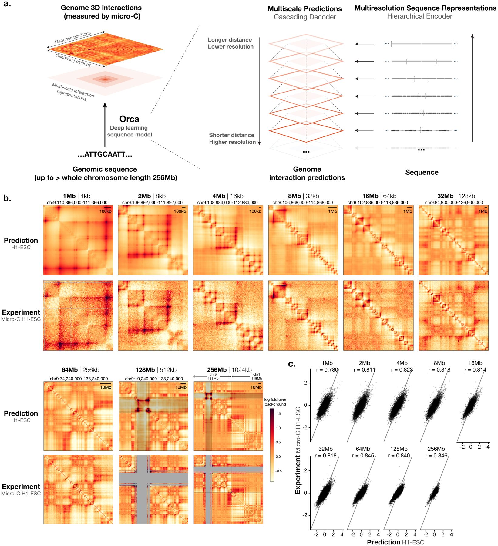
a) Schematic overview of the deep learning model architecture for genome interaction prediction across all scales. Sequence representations at multiple resolutions are computed by a hierarchical encoder starting from the sequence in a bottom-up (high resolution to low resolution) order, whereas genome interaction matrices are predicted from both the corresponding levels of sequence representation and the higher-level genome interaction prediction in a top-down order (low resolution to high resolution). b) Multiscale sequence-based prediction example zooming from the whole-chromosome into a position on a holdout test chromosome. Predictions from 1–256-Mb scales are compared with micro-C experimental observations. Missing values in micro-C data due to lack of coverage are shown in gray, and these regions are also indicated in the 64–256-Mb predictions because the predictions at major assembly gaps or unmappable regions are of unknown accuracy. The genome interactions are represented by the log fold over genomic-distance-based background scores for both the prediction and the experimental data. The predictions for the same regions for the HFF cell type are also shown in Extended Data Figure 1. c). Scatter plot comparison of the predicted interaction scores with the micro-C measured interaction scores on the holdout test chromosomes. 10,000 randomly subsampled scores are shown in each panel. The overall Pearson correlations across the entire test chromosomes are also annotated. Predictions for 1–32-Mb levels are from the Orca 32-Mb model and 64–256-Mb levels are from the Orca 256-Mb model.

The Orca sequence models are capable of predicting diverse genome interaction mechanisms, including not only CTCF-based interactions but also Polycomb-mediated interactions and promoter-enhancer interactions. As illustrated with several regions from the holdout chromosomes, Orca models predicted Polycomb-mediated interactions and promoter-enhancer interactions in a cell-type-specific manner, which are supported by experimental data of interactions and histone marks (Extended Data Figs. 3, 4). The model prediction performances for genome interactions from different genomic region types annotated by CTCF and histone mark ChIP-seq data were also evaluated and compared (Supplementary Figs. 6, 7). This capability of predicting non-CTCF cell-type-specific interactions can potentially contribute to a better understanding of the sequence-basis of cell-type-specific regulation.

Multiscale SV effects on 3D genome predicted from sequence

Since Orca models can accurately predict genome interactions across scales from new unseen sequences, they could be particularly useful when applied to predicting genome variation effects. Notably, because Orca allows very large sequence input (256 Mb, larger than the longest human chromosome chr1: 249 Mb), it enables predicting effects for variants of nearly any size, including very large SVs and copy number variants that are among the most impactful genome variants²⁷. To predict genome structural impact of any variant, one can computationally reconstruct the chromosomal sequence that carries the variant, and compare the predictions against the predictions of the reference sequence. Joint effects of multiple variants on the same haplotype can also be predicted in a similar fashion.

The SV effect predictions of transposon-mediated 2-kb TAD boundary element insertions into various genome locations (2-kb insertion + 5-kb transposon), which have been measured with in situ Hi-C²⁸, were first tested. The insulation score change at each insertion site was computed and compared with the predicted changes. Across 14 insertion sites, Orca attained a cosine similarity score of 0.89 for the H1-ESC model and 0.76 for the HFF model for insulation score changes (P < 1 × 10⁻⁴ for both H1-ESC and HFF, Methods). Moreover, Orca predictions recapitulated all three categories of insertion effects reported, including formation of new boundaries, strengthening existing boundaries, and no domain-level effects (Extended Data Fig. 5, Supplementary Data 2). Thus the experimental Hi-C measurements are highly consistent with the Orca predictions on the genome structural effects of these insertions.

To evaluate the model’s capability in predicting the impacts of diverse types of SVs, the effects of a variety of SVs ranging from 0.3 kb to 80 Mb in size with experimentally measured genome structural impact were predicted (Supplementary Table 3, Fig. 2, Extended Data Fig. 6, Supplementary Figs. 8–14). The multiscale structural impact prediction was first demonstrated with a large 40.5-Mb inversion mutation that was found to be a potential cause of acute myeloid leukemia^29,30, and the predictions were shown at five different levels zooming from a whole chromosome view into the EVI1-proximal breakpoint (Fig. 2a, Supplementary Fig. 8; full predictions at all scales also available at Supplementary Data 3). The predictions showcase both large-scale remodeling of the chromosome organization and the breakpoint-adjacent effects on chromatin compartments and TADs, including at the finest level a gain of EVI1 promoter interaction with a GATA2 enhancer, which has been experimentally confirmed³⁰.

Fig. 2. Multiscale sequence-based prediction of structural variant effects on genome structure.

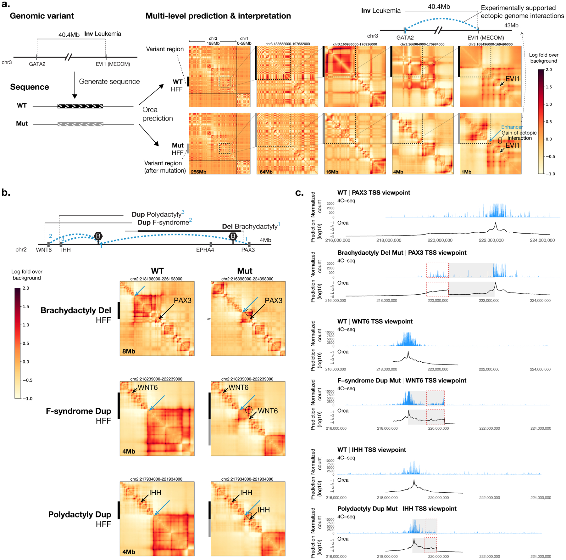
a) Schematic illustration of sequence-based predictions of multiscale genome interaction effects of SVs. A large 40.5-Mb inversion variant involved in leukemia is shown as an example. Predicted effects are shown by predicted genome interaction matrices based on wild type (WT) sequences and mutated sequences (Mut) at multiple scales. The experimentally supported effects of SVs are illustrated at the top of each panel (a-c), with relevant gene positions, major TAD boundaries (marked with the letter B), and range of variant positions indicated (minimal variant range indicated in bold lines). Experimentally supported increase in ectopic interactions is indicated with blue dashed arcs and blue bars. The Orca genome interaction predictions are represented by the log fold over genomic-distance-based background scores. b) Orca predictions of multiple variants with complex phenotypic outcomes in WNT6-PAX3 region. Positions of the major genes affected by the SVs are indicated by black arrows and known enhancer regions involved are indicated by blue arrows. Ectopic interactions caused by the variants are indicated by circles. Black and gray bars on the left side indicate genomic intervals involved in the SVs pre and post mutation. Full multiscale prediction results for both H1-ESC and HFF cell types as well as micro-C observations in the cell types are included in Supplementary Data 3, and validations results for all SVs are summarized in Supplementary Table 3. c) Comparison with 4C-seq experimental data³¹ for variants predicted in b). The normalized counts from 4C-seq and log₁₀ predicted interaction scores (log fold over background) at the 4C-seq point-of-view are shown. The observed and predicted gain of interaction sites relevant to the phenotype are highlighted with the red dashed line box.

Orca predictions were next applied to analyze a complex region where multiple deletion, inversion, and duplication variants ranging from 0.9 Mb to 1.8 Mb lead to several different limb malformation phenotypes: brachydactyly, F-syndrome, and polydactyly³¹. Orca predicts that through different structural alterations all these disease SVs cause de novo contacts between three different genes, PAX3, WNT6, and IHH with the same enhancer region (Fig. 2b–c, Supplementary Fig. 9). These predictions are also fully consistent with prior experimental data based on 4C experiments³¹. These variants showcase several distinct mechanisms that create ectopic interactions predicted by the sequence models: fusion of TADs by boundary deletion creates interactions between distal positions that belonged to two different TADs (PAX3 and the enhancer); duplication creates ectopic interaction between WNT6 and the same enhancer by placing WNT6 sequence into a new context, with similar mechanisms also observed for the Cook syndrome duplications; inversion that spans a TAD boundary leads to changed compositions of both TADs, which results in ectopic interactions of IHH with sequence from a different TAD.

Orca was also applied to complex genomic regions where several adjacent SVs lead to distinct outcomes (Supplementary Figs. 10–14, Extended Data Fig. 6, Supplementary Data 3). The KCNJ2-SOX9 region was first studied, where duplication variants (length 0.2–1.9 Mb) are observed to cause three distinct outcomes: sex reversal (female-to-male), Cooks syndrome (finger hereditary disorder), and no phenotype. Notably, the no phenotype duplication fully encompasses the sex reversal duplication regions. This region has been carefully studied experimentally in³². The effects of both long- and short-form SVs that lead to each phenotype were predicted. Each variant is visualized at a selected scale to showcase their impacts in Figure 2, and the full predictions are available in Supplementary Data 3.

Orca’s sequence-based predictions show that sex reversal duplications (0.2–1 Mb) lead to an enlarged TAD with duplicated interactions with SOX9 within the TAD (Supplementary Figs. 10–12, Extended Data Fig. 6). The duplicated regions include an enhancer³³ in both maximal and minimal duplication variants that cause sex reversal, creating de novo contact between SOX9 and the new copy of the enhancer (Supplementary Fig. 10). In contrast, the larger no phenotype duplication (1.8 Mb) that also includes the RevSex region, is predicted to leave the genome interaction patterns of SOX9 unchanged despite the duplication, because the duplication established a new TAD boundary insulating the new copy from interacting with SOX9. This explains why these duplications lead to the “no phenotype” outcome (Supplementary Figs. 10, 13). A third distinct outcome from disruptions of this region, Cooks syndrome (a finger hereditary disorder), is caused by duplications further extended to include the KCNJ2 gene (1.4–2 Mb). The model predicted that the new copy of KCNJ2 is located in a newly formed TAD due to the duplication, with KCNJ9 hijacking the genome interactions of SOX9. Similar to the no phenotype duplications, SOX9 is insulated in its original TAD and its interactions remain unaffected (Supplementary Figs. 10, 14). Therefore, these results present models of 3D genome architecture changes that explain the phenotypes of those variants, which are fully in agreement with experimental data³². The predictions also provide extra support for the proposed structural changes by resolving ambiguity from the sequencing-based experimental results due to the two duplicated regions being indistinguishable from sequencing reads.

Overall Orca predictions of SV effects were tested on a diverse set of variants across six studies and remarkably in all cases the predictions are concordant with the experimental observations with chromatin conformation capture experiments (Fig. 2, Supplementary Figs. 8–14, Supplementary Data 3, and summarized in Supplementary Table 3). Importantly, such sequence analysis can be made in seconds and is thus scalable to millions or more variants. The accurate recapitulation of genome organization effects of these SVs shows the potential in predicting structural effects of variants without prior data on their consequences in genome 3D structural organization.

Motifs underlie cell-type-specific local genome interactions

The model’s capability in predicting 3D genome architecture at multiple scales directly from sequence also allows to use it as an ‘in silico genome observatory’ to probe the sequence determinants of 3D genome organization learned by the deep learning models. This computational approach has the capability of performing ‘virtual genetic screens’ on a very large number of sequences and allows almost unlimited flexibility in sequence design. Here multiple screen strategies were designed for dissecting the sequence basis of local (1-Mb) and compartment-level (32-Mb) organization, which revealed distinct sequence dependencies.

For discovering sequence dependencies of the sub-megabase scale genome structures that are exemplified by TAD, sub-TAD, and promoter-enhancer interactions, a multiplexed in silico mutagenesis approach was devised to screen for sequence disruptions that lead to ‘local’ structural remodeling within 1-Mb distance (Fig. 3a). This multiplexed approach introduces multiple site-disruption mutations to the same 1-Mb sequence to speed up near-basepair-level screens, leading to 20× speed up in this example. Specifically, each 10-bp site is disrupted in three different sequences each with a random set of disruption sites. Leveraging the sparsity of mutations with structural impact, the site-specific effects were deconvolved using the minimum 1-Mb structural impact score (average absolute log fold interaction changes between the disrupted position and all other positions within the 1-Mb window) across three sequences sharing the same disruption site as the final score (Methods). Taking the minimum of multiple sequences each with independent random disruptions also has the advantage of filtering out the low probability events caused only by specific mutated sequences. We show that this multiplexed approach is highly concordant with the single-mutation approach with >0.9 correlation (Extended Data Fig. 7).

Fig. 3. Identification of cell-type-specific motifs that underlie predicted submegabase-scale genome interactions.

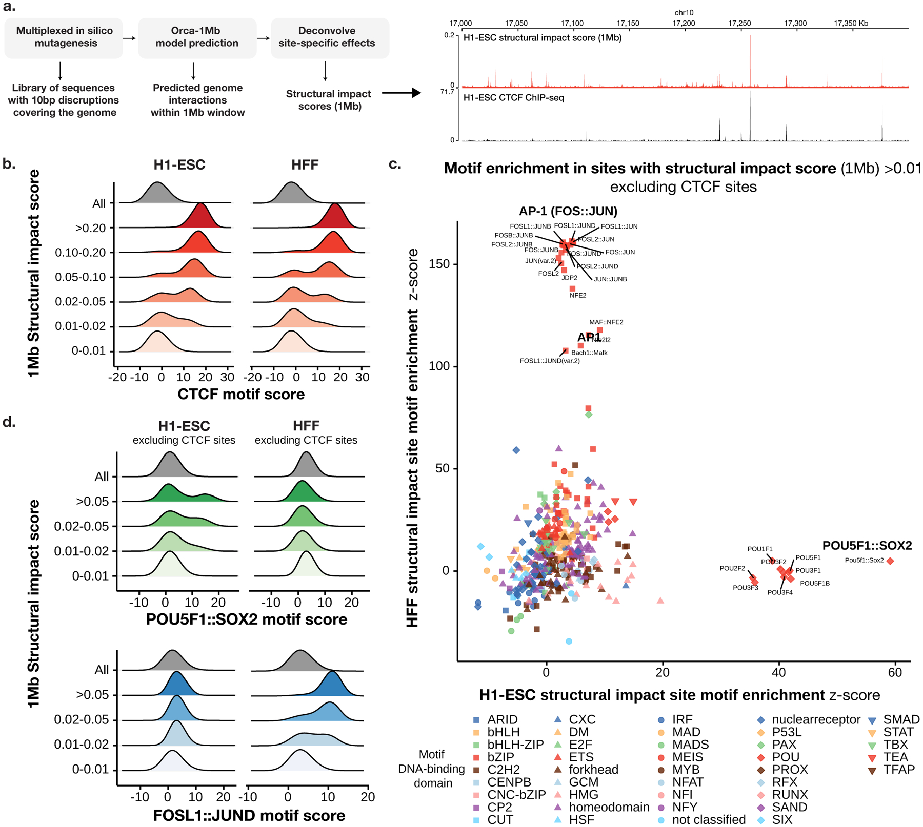
a). Overview of the virtual screen for motif-scale (10-bp) sequences with submegabase-scale structural impact. An example of the estimated 1-Mb structural impact score profile and CTCF ChIP-seq for a section of the genome is shown on the right. b). Distribution of CTCF motif scores (log odds) at 10-bp sequences (including 10-bp flanking sequence) stratified by 1-Mb structural impact score ranges in H1-ESC (left) and HFF (right) are shown. c). Comparison of H1-ESC and HFF structural impact motif enrichment at non-CTCF sites with structural impact scores >0.01. Significance z-scores by two-sided t-test for each motif in both cell types are shown in the scatter plot. Motifs are grouped by DNA-binding domain as in⁴¹. d) Distribution of the cell-type-specific POU5F1∷SOX2 and FOS∷JUN motif scores (log odds) at non-CTCF 10-bp sequences (including 10-bp flanking sequence) stratified by 1-Mb structural impact score ranges in H1-ESC (left) and HFF(right) are shown.

With this approach, all 10-bp sequences on autosomes whose disruptions have structural impact were screened. Consistent with the central role of CTCF in TAD-level structural organization, for both H1-ESC and HFF, most of the 10-bp sites (>88.9%) with the strongest tier of 1-Mb structural impact score (>0.1, <0.015% of the genome) are overlapping with CTCF motifs (log odds > 10) (Fig. 3b) and >95.1% are within 200-bp distance to a CTCF motif (Supplementary Fig. 15), while only <1% are depleted of CTCF motifs (log odds < 6) within 200-bp distance (versus a genome-wide background of 64%). This suggests that the strongest impact sites are predominantly explained by CTCF. However, not all CTCF motifs are predicted to have strong structural impact (only ~1% of sites with CTCF motif log-odds > 10 have structural impact score >0.1), thus CTCF motif is not the only determinant and the model utilizes more complex sequence dependencies to make accurate predictions.

Despite that the strongest tier of 1-Mb structural impact score sites are predominantly CTCF related, non-CTCF transcription factor motifs are highly enriched in the mid-impact score range (0.01–0.1, ~0.2% of the genome), excluding sites with any nearby CTCF motif or binding site (Fig. 3c–d, Methods). Moreover, in contrast to the CTCF motif dependency, which is largely cell-type-invariant (Fig. 3b), very strong cell-type specificity was observed in non-CTCF motifs that are predicted to impact genome structure: H1-ESC is predicted to be most responsive to the disruption of the POU5F1∷SOX2 dimer motif and POU family motifs, while HFF is highly sensitive to AP-1 (FOS∷JUN) motif disruptions (Fig. 3c–d, Supplementary Tables 4, 5, Supplementary Fig. 16; the POU5F1∷SOX2 motif is 48.7× and 1.0x enriched in H1-ESC and HFF, and the FOSL1∷JUND motif is 0.71× and 167× enriched in H1-ESC and HFF, with motif log odds >12). This cell type selectivity is consistent with the well-known gene regulatory roles of POU5F1 and SOX2 in embryonic stem cells³⁴ and AP-1 in fibroblasts³⁵. Example disruptions of single POU5F1∷SOX2 or AP-1 motifs can lead to the elimination of predicted genome interactions in H1-ESC and HFF cell models (Supplementary Figs. 17, 18). These results suggest that cell-type-specific transcription factors mediate local interactions and may also impact transcription through the spatial organization.

A sequence-basis model for compartments with TSS as drivers

As the Orca sequence models uniquely enable the prediction of compartment-level (>1-Mb) genome interactions from sequence, it presents an opportunity to probe into the sequence-based mechanisms of chromatin compartment formation. To understand the sequence dependencies of the compartment-level genome structures as learned by the model, the challenge of deconvoluting sequence effects on chromatin compartments from CTCF-cohesin-mediated mechanisms such as TAD organization needs to be first addressed. To differentiate sequence effects on chromatin compartments, a new sequence model was trained with a cohesin-depleted Hi-C dataset for HCT116 cells³⁶. As acute cohesin depletion completely eliminates TAD domains while chromatin compartments remain intact or strengthened, this sequence model learned only sequence dependencies of chromatin compartments but not CTCF-cohesin dependent structures. The cohesin-depleted HCT116 sequence model predicts genome interactions with a Pearson correlation of 0.71 (32-Mb level, on holdout test chromosomes) and no apparent CTCF motif dependency was observed in this model, consistent with the clean elimination of TADs in this dataset (Supplementary Fig. 19).

To identify the characteristics of sequences that are sufficient for establishing the generally expression-active A or inactive B chromatin compartment according to the model, a virtual genetic screen for ectopic sequence activity in switching A/B chromatin compartment was designed with a strategy of swapping in “insertion” sequences from positions of the genome to a diverse set of target positions (Fig. 4a).

Fig. 4. Virtual screen profiling of sequence-dependencies of chromatin compartments identifies a prominent role of TSS sequences.

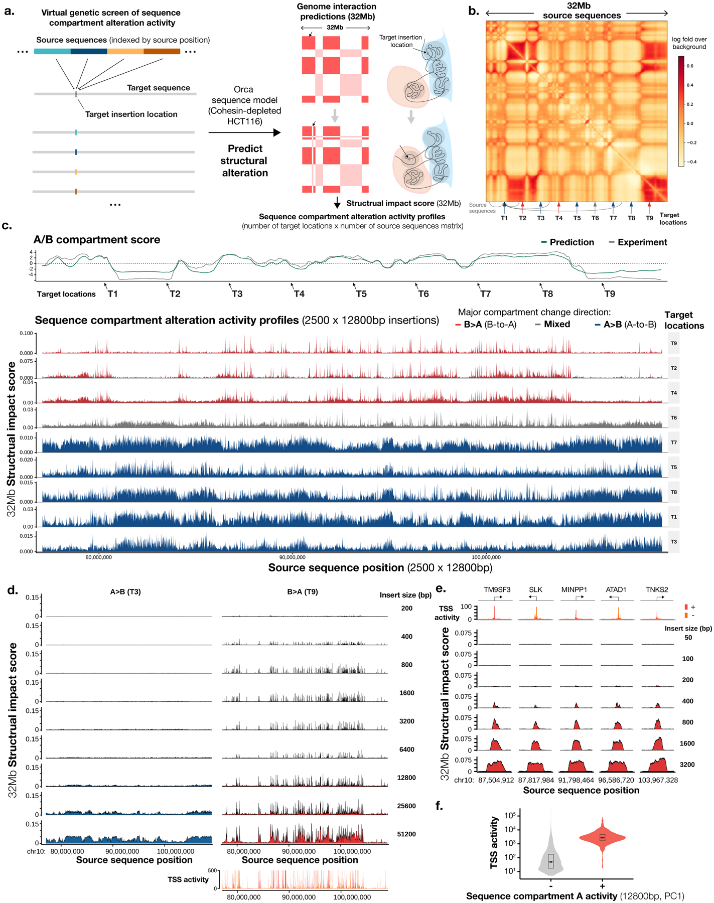
a). Design of the virtual genetic screen for sequence activities in altering chromatin compartment. Source sequences tiling a genomic region or whole chromosomes are inserted into one or multiple target locations by swapping out the original sequence. Genome interaction changes within a 32-Mb window are predicted for each source sequence. b). A virtual screen setup for a region of 32 Mb (chr10:77,072,000–109,072,000), with 9 target locations indicated by arrows and source sequences tiling the entire region. c). Sequence chromatin compartment activity profiles of all source sequences (12,800 bp each) from the 32-Mb region at nine target locations. Top panels show predicted (green) and observed (gray) chromatin A/B compartment scores as computed by the first principal component (PC) of the interaction matrix (high score indicates A compartment). Sequence activity profiles are grouped by the principal compartment change direction of targets: B>A (red), A>B (blue), and mixed (gray). The x-axis shows the locations of source sequences and the y-axis shows the 32-Mb structural impact scores, as measured by predicted average absolute log fold change in genome interactions with the insertion site within the 32-Mb window. d). Effects of insertion sequence sizes (200 bp to 51,200 bp) on chromatin compartment alteration activities, compared at two representative target locations T3 (A>B) and T9 (B<A). Compartment B>A activity is compared with TSS activities as represented by FANTOM CAGE signal (max count across samples). e). High-resolution analysis of sequence compartment A activities at loci with the strongest activities. The x-axis shows the center positions of the insertion sequence and the y-axis shows the 32-Mb structural impact scores. Insert sizes are also annotated. f). Comparison of TSS activities of sequences with and without compartment A activity (top 2% and bottom 98% 12,800-bp sequences, see Methods; total n = 27,281), indicated with ‘+’ sign and ‘−’ sign. The center values of the box plot represent the median; the bounds of boxes represent the 25th and the 75th percentiles; and the notch approximates a 95% confidence interval of the median.

The main characteristics of sequence chromatin compartment activities were here demonstrated with a screen involving a set of 2,500 × 12,800-bp source sequences that tiled a 32-Mb region with multiple A and B compartment regions, and 10 target insertion sites uniformly spaced in the same region (Fig. 4b). For each target site, visualizing the predicted 32-Mb structural impact score (average absolute log fold change in interactions with the insertion site within the 32-Mb window) of all source sequences against the source sequence positions generates a sequence compartment activity profile. These sequence activity profiles are clearly grouped by the compartmental context of the target sites (Fig. 4c, Extended Data Fig. 8, Supplementary Fig. 20): compartment B target sites which detect predominantly B-to-A (B>A) compartment changes and compartment A target sites which detect predominantly A-to-B (A>B) compartment changes, and sites that are near compartment boundaries which detect mixed changes. For succinctness, insertion sequences that are predicted to cause B>A and A>B changes will be referred to as having compartment A activity and compartment B activity respectively.

Sequences with compartment A activities are sparsely distributed in predominantly compartment A regions (Fig. 4c–d, <0.07% of 400-bp sequence have >0.02 32-Mb structural impact score). In contrast, sequences with compartment B activities are widespread across all compartment B regions (Fig. 4c–d). Closer inspection revealed that sequences with strong compartment A activities mostly span transcription start sites (TSS) (Fig. 4d–e). Similar results were recapitulated with a large-scale screen using 12,800-bp insertion sequences tiling all of the holdout chromosomes and 200 random target sites (Fig. 4f, Extended Data Fig. 8, Supplementary Fig. 20). In contrast, the 3’ end of genes are not enriched in compartment A activity (Supplementary Fig. 21). In addition, overlap with HCT116 chromatin states shows very strong enrichment in active TSS states but not in bivalent/poised TSS or other states (Supplementary Fig. 22). Furthermore, little TSS transcription directionality preference was observed in all 200 target positions (Supplementary Fig. 23). A model of active TSS sequences being drivers for compartment A is also in line with prior observations that linked transcription with compartment^4–8. It is worth noting that the cohesin-depleted HCT116 sequence model learned to recognize TSS sequences while training on only 3D genome data without any transcription or chromatin profile data.

The minimum length of insertion sequence that is required for chromatin compartment switching was then assessed using a series of insertion sequence sizes ranging from 200 bp to 51,200 bp (Fig. 4d). Remarkably, insertion of only 800-bp sequence is sufficient for strong A compartment activity, and even 400-bp or 200-bp sequences can have partial effects (Fig. 4d–e). Further increase of length does not significantly increase ectopic compartment A activity until the length starts to cover multiple TSS. While sequences as short as 800 bp are sufficient for the establishment of A compartment within a native B compartment environment, these sequences are expected to induce widespread chromatin changes due to transcription activity or histone modification. For detectable A>B directional compartment change at native A compartment environment, a minimum of 6,400 bp is needed, while 12,800 bp or longer produces more pronounced effects. Interestingly this 6–12-kb minimum length scale coincides with independent experimental measurements of minimum DNA fragment length for maintaining stable compartmentalization. Fragments of at least 10–25 kb are required for stable compartmentalization while <6-kb fragments lead to a gradual loss of genome organization³⁷.

Finally, the size of sequence patterns necessary for compartment activity was analyzed via a permutation-based approach. Specifically, the insertion screen was modified by first dividing the sequence into segments of the same size and then randomly shuffled the order of the segments before insertion, and the effects of different segment sizes are compared. Since permutation eliminates all sequence patterns larger than the specified segment size, if the sequence activity is unaffected after permutation, then such activity only depends upon sequence patterns smaller than the segment size. Interestingly, predicted A-to-B compartment change can be achieved with the insertion of randomly permuted sequences originally with B compartment activity at essentially all segment sizes down to 2 bp (Extended Data Fig. 9). Thus, complex sequence patterns beyond mono- or dinucleotide frequencies may not be necessary for strong predicted B compartment activity (this does not preclude the possibility that some complex sequence patterns can be sufficient for B compartment formation). B compartment activities, before and after permutations, are also correlated with high A/T, low G/C content, as well as AT dinucleotide pattern (Extended Data Fig. 9, Supplementary Fig. 24), which is also consistent with the known enrichment of A/T in B compartment³⁸. In contrast to B compartment activity, compartment A activity is nearly eliminated with segment size below 128 bp and is also decreased at 256 bp, thus A compartment activity likely depends upon sequence patterns of size at least 128–256 bp, which is in line with the involvement of TSS sequences. Moreover, the permuted sequences not only lose A compartment activity but also even gain weak compartment B activity (Extended Data Fig. 9). Consistently, disruption of extended regions of compartment A sequences (e.g. 1.28 Mb) by random permutations are predicted to lead to B compartment formation, while randomly permuted compartment B sequence remains B compartment (Extended Data Fig. 10).

Taken together, these results suggest a sequence-oriented model postulating that chromatin compartment A formation is driven by TSS sequences, likely through induced transcriptional activity and chromatin state changes, while compartment B requires extended sequences (>6–12 kb) without compartment A activity, has a preference to AT-rich sequences, and may be the “default” state established on all non-compartment A sequences.

Discussion

Orca is a sequence model framework for global prediction of 3D genome organization across spatial scales from kilobase to whole chromosomes, based on only genome sequence. It allows the prediction of genome structural impacts of any genome variant including large structural and copy number variants. Orca accurately recapitulated the structural impacts of variants that have previously been experimentally studied. With the potential of rapidly analyzing a large number of variants requiring only the sequences, it can help accelerate the study of structural variants’ roles in health and disease. In addition to enabling predicting variant effects at scale, these sequence models that capture sequence dependencies of 3D genome interaction structures provide new tools for probing sequence-level mechanisms of genome interactions with virtual genetic screens.

As with the multiscale spatial organization of the 3D genome, the sequence dependencies are expected to vary by scale. Sequence determinants at the scale of a single motif appear to be a combination of strong effect CTCF motifs and medium to weak effects that are attributed to tissue-specific TF motifs, possibly through different mechanisms. At hundreds of basepairs length, sequences at TSS are predicted to have activity for establishing compartment A. At 6–12 kb and above, extended stretches of B compartment sequences or even randomly scrambled sequences can establish B compartment. Recently experimentally determined minimal length of genome fragments for maintaining compartment structure is around 6–10 kb³⁷, which is similar to the length scale required to induce significant A>B compartment change. This may suggest this is a key length scale that is required for the underlying biophysical mechanisms of compartmentalization, possibly through phase separation.

From a sequence-based perspective, compartment A appears to be the ‘active’ compartment that requires specific sequence patterns, as widespread chromatin changes may be induced with the insertion of TSS-proximal sequences. In contrast, compartment B appears to be the ‘passive’ compartment as it requires extended sequences without compartment A activity, and compartment B structures are predicted to be robust to random permutation of sequence. Note that the notion of ‘active’ or ‘passive’ here indicates only the sequence dependency characteristics but not the molecular mechanisms, as establishment and maintenance of both compartments could involve active molecular biochemical activities. These hypotheses remain to be tested through future experiments. Moreover, further studies may extend or revise sequence dependencies of chromatin compartment that are proposed in this model, such as possible dependencies on sequences that activate or repress transcription.

There are a few limitations of this study that are worth mentioning. Even though the predictions closely recapitulate experimental observations in most cases, in some cases they still differ from observation beyond what can be explained by technical noise or alignment artifact as shown in Supplementary Data 1. Thus, there is still space for further improvement in performance, and new sequence-based mechanisms are expected to be discovered with higher resolution data and improved models. Secondly, machine-learning-based approaches like Orca are expected to capture sequence pattern dependencies that recur across the genome, therefore sequence-based mechanisms that uniquely apply to very few or even a single genomic locus may not be learned through this approach. Thirdly, sequence models may face challenges in learning the correct “driver” sequence patterns when the “passenger” sequence patterns are nearly perfectly correlated with the driving factor, even though the model can identify the correct driver when the correlations are less perfect and the training data are sufficiently informative. Lastly, because of the current limitation in measuring structure for highly repetitive regions from Hi-C reads, the model’s prediction in these regions were unable to be rigorously assessed (the model typically predicts B compartment-like structure for these regions). Complete end-to-end assembly of the human genomes³⁹ and long-read sequencing techniques⁴⁰ may allow addressing this limitation in the future.

The Orca sequence models also provide ample new opportunities for designing sequence-based experiments to probe sequence dependencies of 3D genome organization with ‘virtual genetic screens’ beyond what was explored in this manuscript, such as finely dissecting sequences at basepair resolution for interactions at specific loci. Such analyses can be done with the models and code released here. More generally, I anticipate such deep learning model-based approaches for in silico modeling of complex biological processes to be powerful methods to generate hypotheses for biological systems.

Methods

Orca model architecture for multiscale 3D genome prediction

The Orca model architecture is composed of a hierarchical sequence encoder and a multi-level cascading decoder, designed to provide a “zooming” series of predictions at multiple scales (Fig. 1). The hierarchical sequence encoder transforms a large input sequence up to 256 Mb to a series of sequence representations at multiple resolutions. A series of cascading decoders each predicts an interaction matrix, which represents all pairwise genome interactions within a window of varying sizes from 1–256 Mb at different resolutions. All predicted interaction matrices are of size 250 × 250 and all predicted scores represent log fold over distance-based background. Decoder at each level takes the sequence encoding at the corresponding resolution as input. The top-level decoder receives input from the entire sequence at the lowest resolution, and lower levels receive sequence representations at higher resolutions. For example, 32-Mb level decoder receives 128-kb resolution sequence encoding for 32-Mb sequence and 1-Mb level decoder receives 4-kb resolution sequence encoding for 1-Mb sequence. In addition, except for the top-level decoder, lower-level decoders also receive the prediction from the upper level as input (e.g. 1-Mb level decoder receives 2-Mb level prediction, cropped to the 1-Mb region), and all multi-level decoders also receive a distance encoding matrix as input. The encoder computation starts from a bottom-up pass (high resolution to low resolution) starting from raw sequence with one-hot encoding, followed by a top-down pass to introduce longer range information to the finer-resolution representations (Supplementary Fig. 1). The decoder computation follows a top-down order (long maximum distance to short maximum distance, low resolution to high resolution) and each lower-level decoder receives the upper-level prediction as input. The architecture and input were described in more detail below, and the detailed architecture of models is available in Supplementary Figure 1 and the code repository.

Both the encoder and decoders are convolutional networks with residual connections. The hierarchical sequence encoder alternates between 1D residual convolution blocks and max-pooling layers. More specifically, the first section of the sequence encoder converts the one-hot sequence encoding into 4-kb resolution sequence representations with a convolutional architecture adapted from Sei⁴² that uses a dual linear+nonlinear path design that stacks nonlinear blocks with residual connections on top of the linear blocks (Supplementary Fig. 1). The first section of the encoder contains 28 convolution layers each with 64–128 channels. With the 4-kb resolution sequence encoding as input, the upper sections of the encoder create a series of sequence encoding at 4-kb, 8-kb, …, 1024-kb resolutions with factors of 2 with a similar residual block structure, using 4 convolution layers per resolution with 128 channels.

To predict 2D interaction matrices at multiple scales, a cascading series of sequence decoders was used, each predicting a genome interaction matrix with a different length and resolution. The 2D convolution architecture consists of 2D residual convolution blocks with the linear+nonlinear path design. The 2D convolution blocks cycle through dilation factors of 1, 2, 4, 8, 16, 32, 64 for four full passes with a total of 112 convolution layers per decoder. Decoders at lower levels receive input from the corresponding level of sequence representations, the interaction matrix prediction from one-level above, and a 2D pairwise distance encoding matrix as an auxiliary input. 1D sequence representations are transformed to 2D with the pairwise sum operation (Y_ij = X_i + X_j). The lower-level decoders predict for a sub-region half the window size of the upper-level prediction, and the prediction from the upper-level corresponding to this region was upsampled by a factor of 2 and provided as input. For the distance encoding matrix D, for each cell type, D_ij is the log distance-based expected balanced contact score at each genomic distance |i − j| for intrachromosomal pairs {i, j}, and interchromosomal pairs are filled with a constant of average interchromosomal log expected balanced contact score. The distance-based expectation scores for 32–256 Mb were monotonically transformed so that the scores for longer distances are no higher than the shorter distances. The distance encoding matrix and the upsampled prediction from the upper level are combined with the 2D sequence representation by concatenation followed by a convolution block (Supplementary Fig. 1). The final model prediction is symmetrized by averaging with its transpose. The model predictions are averaged between the predictions from the forward and the reverse-complement sequences.

The sequence encoder is also trained with an auxiliary task of predicting DNase-seq and ChIP-seq chromatin profile labels (Supplementary Table 6) which improved performance. To simultaneously predict chromatin profile labels and genome interactions, a 1D convolution block for predicting chromatin profiles is introduced which receives input from the 4-kb resolution output of the sequence encoder.

Model training and evaluation

The processed micro-C datasets for H1-ESC and HFF cells¹⁵ were downloaded from the 4D Nucleome (4DN) data portal (accession IDs 4DNFI9GMP2J8 and 4DNFI643OYP9). The genomic sequences were retrieved from the GRCh38/hg38 reference genome. Training data were generated on-the-fly during training by uniformly sampling the genome from training chromosomes with the Selene deep learning sequence modeling library²¹. A separate model was trained for each micro-C dataset. The on-the-fly sampling generated new training samples for every training step. Each training sample consists of a sequence (the input) and the corresponding multi-level distance-normalized contact matrices (the target), which was also referred to as the genome interaction matrices. To compute the genome interaction matrices, the iterative correction matrix balancing algorithm⁴³ and adaptive coarse graining procedures were applied to the contact matrices retrieved from the micro-C datasets with cooler and cooltools packages²⁶. Adaptive coarse graining is a preprocessing procedure implemented in the cooltools package that smooth the low coverage areas of the contact map with adaptive window size and this step eliminates zeros by pooling the reads from the local neighborhood. No further smoothing was applied to preserve the spatial resolution of the data. The processed matrix was then divided by the background matrix which is the exponential of the distance encoding matrix as described in the previous section (all operations are elementwise), and the minimum value of the background matrix was added to both nominator and denominator for numerical stability and noise reduction. The distance-based expectations are computed per chromosome with cooltools and then aggregated over all chromosomes. The distance-expectation curve beyond a 1.6-Mb distance is smoothed with lowess. The chromosomes were divided into the training set (all chromosomes except for chr8, 9, and 10), the validation set (chr8), and the test set (chr9, 10).

The main loss function is the mean squared error between the predictions and the targets, or $\frac{1}{N}{\Vert \text{prediction – target}\Vert }_2^2$, where prediction and target are both 250 × 250 square matrices, N indicates the number of elements in the matrix to average over, and the norm sign indicates the Frobenius norm. Missing values in the genome interaction matrices, which are typically due to low or no coverage, are ignored in the loss and gradient computation. An auxiliary binary cross entropy loss function is also used to train the 4kb resolution sequence encoding to simultaneously predict DNase-seq and ChIP-seq chromatin profile labels, or specifically the auxiliary loss is $\frac{1}{N}{\text{[target}}_{\text{c}}\cdot {\text{log(prediction}}_{\text{c}})+\left(1-{\text{target}}_{\text{c}}\right)\cdot {\text{log(1-prediction}}_{\text{c}})]$ where target_c are binary chromatin profile target matrix of size d × 250 (d is the number of chromatin profiles), and the predicted probability matrix of the same size, and N is the total number of elements in the matrix. The auxiliary loss is simultaneously trained on the same set of sequences as the main loss function. The list of chromatin profiles used is provided in Supplementary Table 6. The chromatin profile labels are generated for 4-kb bins and labeled one or zero based on whether any peak overlaps with the 4-kb bin.

To allow training large-scale sequence models that do not fit into GPU memory with standard techniques, a horizontal checkpointing method was devised leveraging the hierarchical structure of the model (see Methods section “Scaling hierarchical deep learning model training” for details). Other training optimizations include parallelizing training data generation on CPU and randomly selecting either forward or reverse-complement sequence for prediction, which can be seen as an unbiased stochastic approximation to averaging predictions from forward and reverse-complement sequence.

For both flexibility in model application and efficiency in model training, the model was designed to be composed of three stackable modules (1 Mb, 1–32 Mb, 32–256 Mb), which were trained in three stages. In the first stage, the sequence encoding at 4-kb resolution was pretrained with the task of predicting genome interactions within 1-Mb distance at 4-kb resolution and the auxiliary task of predicting chromatin profile labels at the same resolution (the cohesin-depleted HCT116 model was trained without auxiliary task). The encoder up to 4-kb resolution and the decoder trained in the first stage is also called Orca-1Mb. In the second stage, with the pretrained first section of the sequence encoder from the 1-Mb module, the multiscale 1–32-Mb model was trained to predict at 1-Mb, 2-Mb, 4-Mb, 8-Mb, 16-Mb, and 32-Mb levels. For training multiscale prediction models, a series of subregions with increasingly smaller window size and finer resolution at each level, or the ‘zooming’ series, was selected. For example, for a 32-Mb sequence, a 16-Mb subregion was randomly selected, then an 8-Mb subregion within the 16-Mb region was randomly selected and continue until a 1-Mb region was selected. The encoder up to 128-kb resolution and decoders trained in the second stage are also called Orca 2-Mb. In the third stage, the 32–256-Mb model is trained for both intrachromosomal and interchromosomal interactions, with the pretrained sequence encoder up to 128-kb resolution from the 1–32-Mb model. The full encoder and the third stage decoders are also called Orca 256-Mb. The training data for 32Mb–256Mb model were sampled from multiple chromosomes with the following process: a chromosome was first sampled, add the full length of that chromosome to the sequence; then sample another chromosome, add the full length chromosome if not exceeding 256 Mb, otherwise sample a subregion on that chromosome that make up a total of 256 Mb; continue adding new chromosomes until 256-Mb sequence is filled; randomly permute the order the sequence segments sampled and randomly select a strand direction for each segment; retrieve the corresponding sequence, intrachromosomal and interchromosomal genome interactions, and distance encodings as described above. The training process with stochastic gradient descent took about 480,000 steps for the first stage (1-Mb sequence and batch size 16, learning rate 0.002 with momentum 0.98, and the last 1/3 of steps are trained with stochastic weight averaging⁴⁴), 150,000 steps for the second stage (32-Mb sequence with batch size 4 and learning rate 0.001 with momentum 0.98), and 20,000 steps for the third stage (256-Mb sequence with batch size 4 and learning rate 0.001 with momentum 0.98). The training hardware was one server equipped with four NVIDIA Tesla V100 32GB GPUs. The code for training Orca models with full details of the implementation is provided at the code repository.

Each training stages generates training data from micro-C data processed to different resolutions. The training data was sampled from the micro-C contact matrices at 1-kb resolution for the 1-Mb model, 4-kb resolution for the 1–32-Mb model, and 32-kb for the 32–256-Mb model, and these high-resolution matrices are downsampled to the prediction resolutions of the decoders. Downsampling is performed by taking the average of the multiple entries that are collapsed into one, excluding the missing values. To further reduce overfitting, the input sequences for training are shifted by a random offset within 100 bp for the 1-Mb model, 1 kb for the 1–32-Mb model and 4 kb for the 32–256-Mb model.

Model prediction evaluation on holdout test chromosomes

To evaluate the model prediction performance on holdout test chromosomes, multiscale genome interaction matrices were systematically predicted on the test chromosomes and the predictions were compared with the observed micro-C data. The evaluation data were processed in the same procedure as for training data generation. Missing values in the micro-C target matrices are excluded from the evaluation (missing values are typically due to low or no coverage). Because target matrices at lower resolutions are downsampled from higher resolution matrices by the binning procedure described above, a downsampled value is computed from averaging multiple values from high resolution matrix while excluding missing values, and if >25% of these values are missing then the downsampled value is also skipped in evaluation. Specifically, for evaluating the predictions at 1–32-Mb levels the test set chromosomes were tiled with 32Mb windows at a step size of 0.5 Mb. For each 32-Mb window the genome interactions were predicted at all scales from 1 Mb to 32 Mb by sequentially zooming into 16-Mb, 8-Mb, 4-Mb, 2-Mb, 1-Mb sub-windows each located at the center of the higher level region. All prediction matrices were concatenated and flattened, and Pearson correlation was computed between the predictions and micro-C observations. The 1-Mb level performance of the 1–32-Mb models was also compared with the 1-Mb module predictions on the same 1-Mb windows.

For evaluating the intrachromosomal 32–256-Mb scale predictions, two 256-Mb sequences each containing a test chromosome were first generated, with the rest of the 256-Mb length padded with sequence from chr1 (only the intrachromosomal interactions were evaluated). For predictions at 128-Mb, 64-Mb, and 32-Mb levels, the same starting positions that tile the test chromosomes with step size of 5,120 kb were used. Windows that extend beyond the test chromosome boundaries were discarded from evaluation.

For evaluating interchromosomal predictions for 32–256-Mb scale predictions, multichromosomal 256-Mb sequences were constructed by randomly sampling sequence segments from test chromosomes and concatenation. Specifically, the length of each sequence segment was uniformly chosen at random between 64 to 128 Mb, and the last segment is truncated to 256 Mb when the total length exceeds 256 Mb, then the orders of the sampled segments are randomly shuffled. Distance encoding matrices are constructed accordingly. 100 sequences of 256 Mb are constructed and multiscale predictions zooming into the center of each 256-Mb sequence were generated (128-Mb, 64-Mb, 32-Mb regions at the center of each 256-Mb sequence are selected). Only interchromosomal predictions are evaluated.

For comparison with Akita²³ on submegabase-scale predictions, predictions from Akita were generated on its test set samples that are also located in Orca test chromosomes 9 and 10. Orca predictions for the same genomic regions were then generated with the Orca 1–32-Mb models and only predictions at the 1-Mb level were used. The Orca 1-Mb-level predictions and target genome interaction matrices are resized using bilinear upsampling with a factor of 2 and cropped to the Akita output region, and additional Gaussian filtering with sigma 1 and kernel size 5 and clipping to (−2, 2) was then applied to match the Akita data processing step. For each test sample, background-subtracted Pearson correlations were computed against the Akita targets and Orca targets processed as described above. To compute background-subtracted Pearson correlation, for any prediction or target matrix, each score was subtracted by the average scores at the same distance in the same matrix before computing correlation. The background subtraction has minimal effects on preserving the genome structure information and improved robustness to different data preprocessing.

Scaling hierarchical deep learning model training

To scale deep learning sequence models to hundreds of megabases, a scalable memory-efficient training algorithm was devised to dramatically reduce the memory requirement. As illustrated in Supplementary Figure 25, the regular training procedure for deep learning is layer-wise and stores all internal representations in memory for computing gradients, which results in extremely high memory demand for large model input. Checkpointing is a memory-saving technique first developed for residual networks with a high number of layers⁴⁵. With checkpointing, only internal representations at the checkpoint layers are stored and other internal representations can be recomputed on-the-fly when gradient computation is needed. However, even with the checkpointing technique, training is still infeasible for very large sequence input because the memory requirement of computing even only the first layer for a single sequence is beyond the maximum capacity of currently available GPUs.

Leveraging the hierarchical structure of the sequence model, the memory consumption of the bottom layers, which use the most memory, can be greatly reduced by executing them in horizontal blocks and only store the output of the blocks. This approach fixed the memory usage of the lower layers to the memory needed to compute the block, with the minimum block size being the receptive field of the block output layer (recommended sizes are at least two folds of the minimum for computational efficiency). For example, the receptive field of 4-kb resolution layer output of the Orca sequence encoder is 212 kb, which is less than 1/150 of 32 Mb or 1/1200 of 256 Mb, allowing great reduction of memory usage. Because the memory consumption in the bottom layers is orders of magnitude larger compared to the upper layers, this essentially resolved the memory consumption issue for Orca models and allowed us to scale to and beyond whole-chromosome-scale input. I refer to this technique as horizontal checkpointing. Horizontal checkpointing was used to allow the model to scale to large input for training and prediction of Orca 32-Mb and Orca 256-Mb models. Horizontal checkpointing also allows gradient computation during model training, and while this capability was not utilized in the current models due to the increased training time, such capability can be useful in future studies.

Structural variant impact on multiscale genome interactions

Orca models allow the prediction of the multiscale genome organization impact of almost any genome variant at any size. This is naturally achieved by comparing the model predictions of chromosomal sequences of the reference allele and the alternative allele. The capability of using up to 256 Mb as input allows the analysis of even very large variants as well as including large context sequence up to the whole chromosome. This approach is also extendable to analyzing the joint effects of multiple variants in the same haplotype or even whole individual genomes. Specifically, to predict the structural impact for each variant, multiple series of multiscale prediction were generated, each zooming into a breakpoint introduced by the variant in the alternative allele sequence, or their corresponding positions in the reference sequence.

For prediction of transposon insertion effects, the sequences after insertions were computationally generated based on Zhang et al.²⁸. Experimental in situ Hi-C data that measured the insertion effects were also obtained from the same study. To quantify the insertion effects by insulation score changes (Mut-WT), the insulation score is measured as the average intra-region interaction (cis) for the two 200-kb regions before and after the insertion site, subtracted by the average inter-region (trans) interaction scores between the two regions (Extended Data Fig. 5e). The interaction scores are quantified by log fold over distance-based background. Cosine similarity was used to compare the predicted and observed insulation score changes across 14 insertion sites (two sites, C21S8 and C21S9 are excluded because of missing values in the in situ Hi-C data). P values are computed with an empirical null distribution of 100,000 cosine similarities between the same predicted insulation score changes and experimental insulation score changes by randomly flipping WT and Mut labels for each insertion site.

Multiplexed in silico mutagenesis

To systematically identify sequences underlying submegabase-scale genome interactions at the single motif scale, an in silico mutagenesis approach that uses the Orca sequence models to predict the effects of a large number of mutations that cover the genome was designed. In this study, a score was assigned to all genomic sequences in 10-bp bins on autosomes representing the structural impact of its disruption. To perform a genome-scale screen, the analysis was sped up by introducing a multiplexed approach to in silico mutagenesis. Since 10-bp sequences with strong structural impacts are sparse (most disruptions have near zero effects), multiple random disruptions can be introduced to the same sequence with a very low probability that more than one disruption will have a strong effect. The multiplexed design ensures that for each 10-bp sequence multiple random disruptions are introduced in different sequences each with a different set of random disruptions. The 10-bp site-specific sequence disruption effect was then deconvolved by taking the minimum effect of all sequences that carry a disruption of the 10-bp sequence. The disruption impact on local genome interactions is measured by 1-Mb structural impact score, which is the average absolute log fold change of interactions between the disruption position and all other positions in the 1-Mb window. The Orca 1-Mb modules for H1-ESC and HFF are used for all predictions to allow fast screening of a large number of sequences.

More specifically, the genome was tiled with 1-Mb windows at 0.8-Mb step size across all autosomes. Each 1-Mb window is considered as 25 × 40-kb regions each containing 4,000 × 10-bp disruption sites. 12,000 mutated sequences are generated for each 1-Mb window. Each generated sequence contains 20 disruptions in each of the center 20 × 40-kb regions. Each 10-bp is disrupted in three different sequences. This multiplexed design can be generated by assigning all 10-bp sequences to a 20 × 4,000 matrix with each row containing all 10-bp sites of a 40-kb region, then randomly shuffle each row independently, resulting in 4,000 columns each corresponding to a mutated sequence. This process was repeated three times to generate 12,000 sequence designs. According to these designs, 10bp sequence disruptions are introduced by replacing the original 10-bp sequence with random nucleotides that match the nucleotide composition in the 1-Mb window.

For motif enrichment analysis, vertebrate non-redundant motifs were downloaded from the JASPAR database⁴⁶. Motif matches for each 10-bp site were scanned for after extending by 10-bp flanking sequence on each side, and a maximum log-odds score over the 30-bp window for each motif was obtained. The maximum motif log-odds score in this window was also referred to as the maximum motif log-odds score for the 10-bp site. To avoid overlap of extended sequences, only one 10-bp site every 30-bp was considered for statistical tests. To analyze non-CTCF motif enrichments, 10-bp sites with 1-Mb structural impact score > 0.01 and without nearby CTCF motif matches (CTCF max motif log odds < 6 within 200 bp) or CTCF binding sites (CTCF ChIP-seq fold over control < 4; ENCODE accession IDs ENCFF473IZV, ENCFF761RHS) were used. Next, to quantify the enrichment of motifs, two-sided t-test (without assuming equal variance) was performed to compare the motif log odds scores of these filtered sites, against the background of 100,000 sites random drawn among all 10-bp sites screened. Fold enrichment was also computed on the same sites with a motif log odds threshold of 12.

For pileup analysis of H1-ESC and HFF micro-C datasets at POU5F1∷SOX2 and FOS∷JUN structural impact sites, the average interaction matrix (log fold over background scores within 1-Mb window) centered at all non-CTCF sites (as defined above) across the genome with motif log odds >10 and >0.02 1Mb structural impact score for the same cell type that matches the micro-C datasets was computed. For pileup analysis of CTCF structural impact sites, similarly the average over all sites of CTCF motif log odds > 10 and 1-Mb structural impact score > 0.1 was computed.

Virtual genetic screen for chromatin compartment activity

For performing virtual screens of sequence chromatin compartment activity, an Orca model was first trained for the cohesin-depleted (after 6h auxin treatment) in situ Hi-C HCT119 dataset³⁶, in which the TADs were eliminated while chromatin compartments were intact or strengthened. The dataset was downloaded from the 4DN data portal (accession ID 4DNFILP99QJS). The cohesin-depleted HCT119 Orca model was trained from scratch with a similar procedure as described above, with a difference that the HCT119 model was trained without the auxiliary loss function of predicting DNase and ChIP-seq chromatin profiles at any stage of training.

To screen for sequence activity of chromatin compartment alteration, a virtual screen with ectopic insertions of genomic sequences was designed. For each screen, a pool of source sequences and one or more target positions were selected. For every source sequence and target location pair, the source sequence was “inserted” into the target location by swapping out the original sequence at the target position, then the genome interaction pattern changes were predicted and quantified by the 32-Mb structural impact score (the average absolute log fold change of interactions between the target position and all other positions in the 32-Mb window). Because a large proportion of the mutated sequence is in common with the original sequence, the computation was sped up by only recomputing the internal representations that are affected by the change.

The source sequences were generated from a large genomic region or across entire chromosomes by dividing the region into fixed-sized segments, and the structural impact scores of the source sequences at all positions were visualized as a chromatin compartment alteration activity profile. For exploratory virtual screens, a 32-Mb region chr10:77,072,000–109,072,000 covering multiple A compartment, B compartment, and intermediate regions was used. Activities of source sequences tiling this region were screened for at 9 target positions that are uniformly spaced in the same region. For the large-scale screen, source sequences with 12,800-bp length tiling all of the holdout chromosomes chr8, 9, and 10 were used, with sequences overlapping with blacklisted regions removed. Here the blacklisted regions were defined as 4-kb genomic bins with missing values in the Hi-C datasets used in this manuscripts, or with more than 10 unknown bases (“N”s) in the reference genome sequence. 200 target positions spanning all holdout chromosomes are randomly chosen from source sequence start positions. The 32-Mb windows for Orca prediction in the large-scale screen are centered at the target positions. After performing the screen, the A/B chromatin compartment activity of each 12,800-bp sequence was quantified, by taking the first principal component across the 200 compartment activity profiles (one for each target position). The sign of a principal component is arbitrary, but the direction that corresponds to compartment A activity can be easily detected, such as based on TSS enrichment. The top 2% sequences with strongest compartment A activity were used for downstream enrichment analysis.

For enrichment analysis of the chromatin compartment activities, the FANTOM CAGE signal profile (maximum count across samples) was downloaded from the UCSC table browser with a filter of count >1, and the annotations for TSS, 5’UTR, 3’UTR, exon, and genes were from Ensembl release 97. The chromatin state annotations for HCT116 are from EpiMap⁴⁷.

For performing analyses with random permutation of sequences, the sequence to be permuted was first divided into segments of the same specified length, then the order of the sequence segments were randomly permuted. As random permutation disrupts any sequence patterns larger than the segment length, this analysis can be used to reveal the length scale of the sequence dependencies.

Extended Data

Extended Data Fig. 1. Performance of Orca model predictions for the HFF cell type.

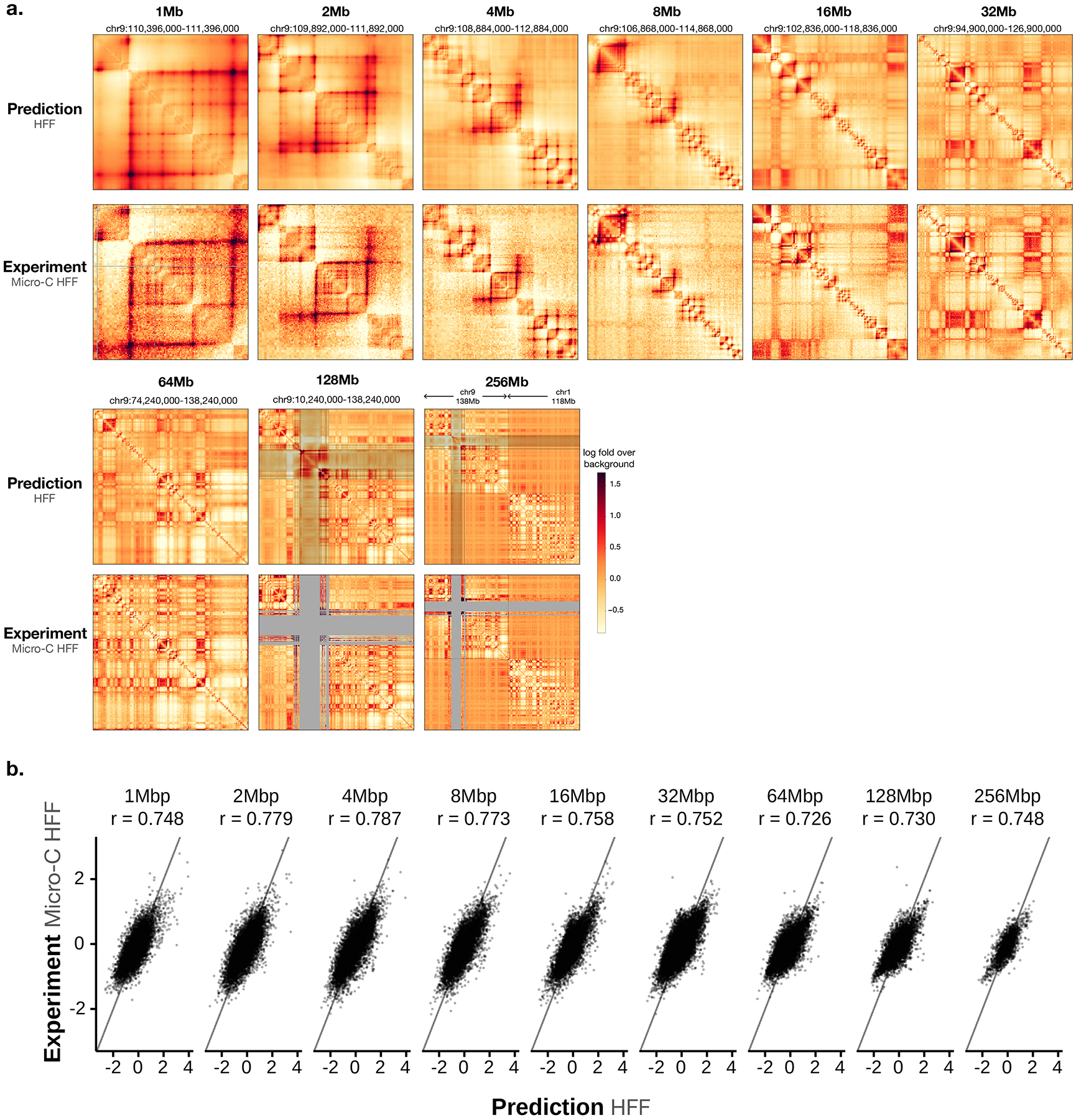
a). A multiscale sequence-based prediction example zooming from whole-chromosome into a position on a holdout test chromosome. Predictions from 1–256Mb scales are compared with micro-C experimental observations. Missing values in micro-C data are shown in gray, and these regions are also indicated in the 64–256Mb prediction heatmaps because predictions at major assembly gaps or unmappable regions are of unknown accuracy. The genome interactions are represented by the log fold over genomic-distance-based background scores for both prediction and experimental data. b). Scatter plot comparison of the predicted interaction scores with the micro-C measured interaction scores (log fold over background) on the holdout test chromosomes. 10,000 randomly subsampled scores are shown in each panel. The overall Pearson correlations across the entire test chromosomes are annotated. The genome interactions are represented by the log fold over background scores for both prediction and experimental data. Predictions for 1–32Mb levels are from the Orca-32Mb model and 64–256Mb levels are from the Orca-256Mb model.

Extended Data Fig. 2. Performance of Orca model predictions for cross-cell-type genome interaction difference.

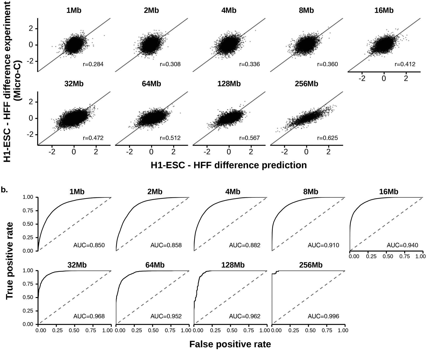
a). Scatter plot comparison of the predicted cell type differences of genome interactions (HFF - H1-ESC) with the micro-C measured interaction score differences on the holdout chromosomes. 10,000 randomly subsampled scores are shown in each panel. The overall Pearson correlations across the entire test chromosomes are annotated. The genome interactions are represented by the log fold over genomic-distance-based background scores for both prediction and experimental data. b). Prediction performance for position pairs with the strongest absolute log-fold differences between the two cell types (top 1 percentile). The performance of models predicting the cell type labels (the cell type with stronger interaction) is measured by receiver operating characteristic (ROC) curve. The area under the ROC curve (AUROC) is annotated. The AUROC score can be interpreted as the probability of a randomly selected positive example (i.e. stronger in HFF) being ranked higher than a randomly selected example (i.e. stronger in H1-ESC). Predictions for 1–32Mb levels are from the Orca-32Mb models and 64–256Mb levels are from the Orca-256Mb models.

Extended Data Fig. 3. Example Orca predictions of Polycomb-mediated interactions.

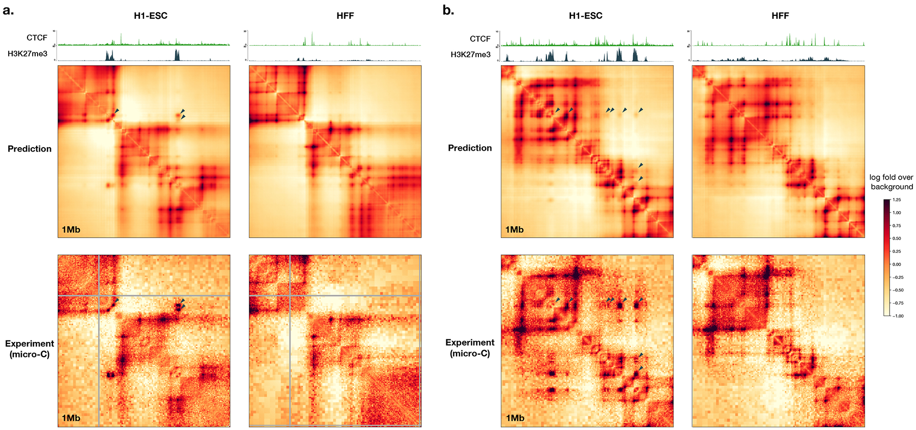
Predicted and observed H1-ESC and HFF genome interactions for two regions from a holdout chromosome, a). chr10:116850000-117850000 and b). chr10:100450000-101450000 are shown. The predicted and observed Polycomb-mediated interactions are marked with black triangles. ChIP-seq signal tracks for CTCF and H3K27me3 for the two cell types are also shown. Polycomb-mediated interactions are predicted to be specific to H1-ESC in both examples, consistent with experimental micro-C and ChIP-seq data.

Extended Data Fig. 4. Example Orca predictions of promoter-enhancer interactions.

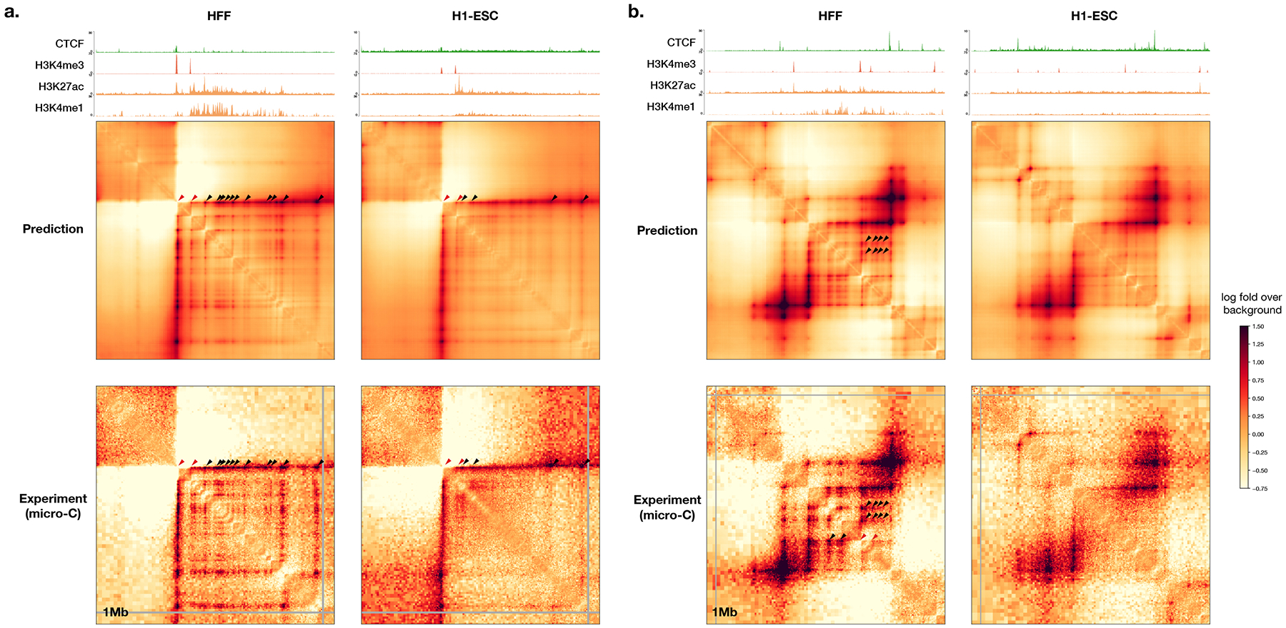
Predicted and observed H1-ESC and HFF genome interactions for two regions from holdout chromosomes, a) chr8:127400000-128400000 and b) chr9:94360000-95360000 are shown. The predicted and observed enhancer-promoter interactions are marked (promoter positions or promoter-promoter interactions are marked with red triangles, enhancer-promoter or enhancer-enhancer interactions are marked with black triangles; we only marked a subset of all interactions observed). ChIP-seq signal tracks for CTCF and H3K4me3, H3K27ac, and H3K4me1 for the two cell types are also shown. The predicted enhancer-promoter interactions are consistent with micro-C observations and enhancer histone mark signal from ChIP-seq data.

Extended Data Fig. 5. Visualized predictions of transposon-mediated boundary element insertion effects in multiple insertion sites.

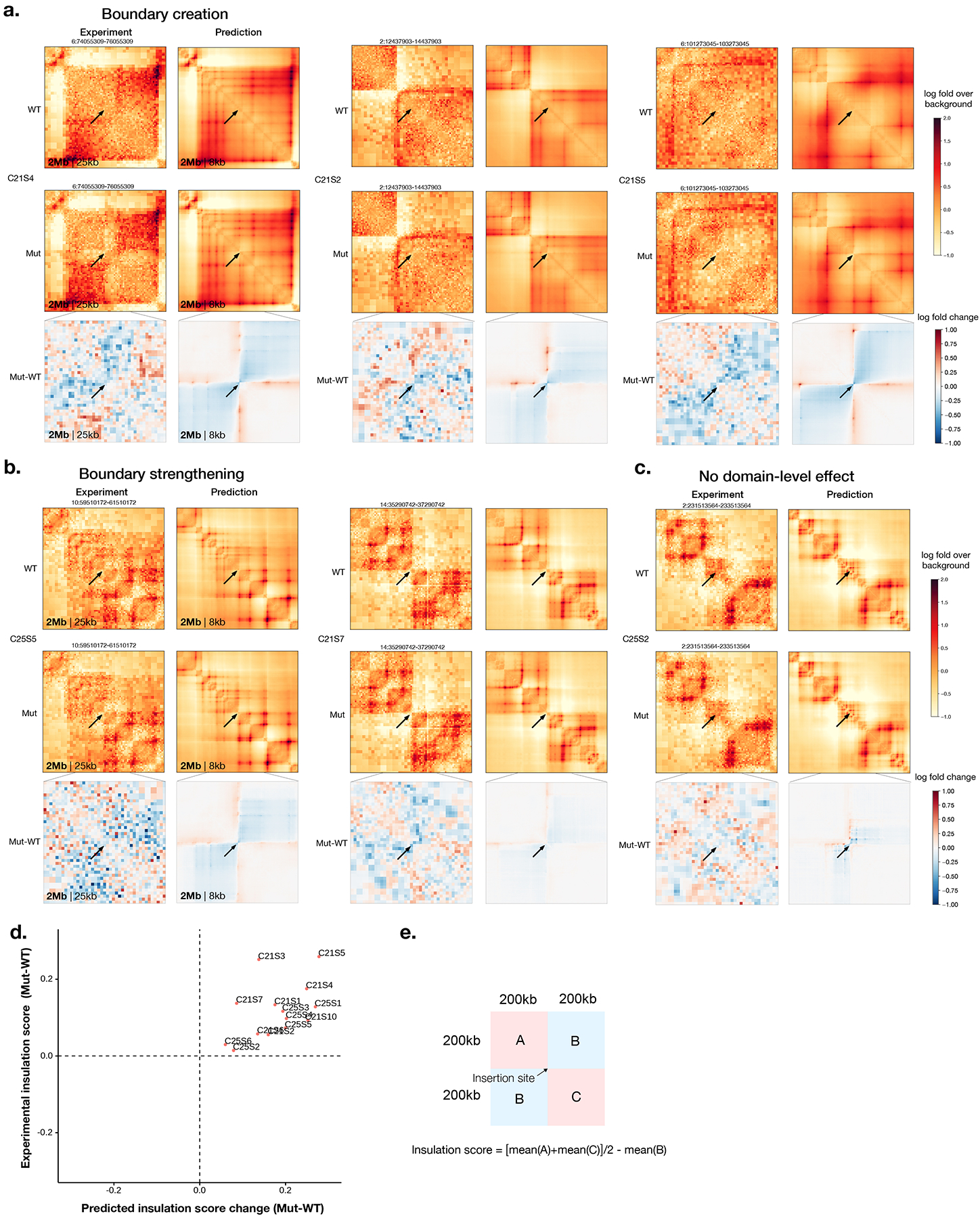
All insertions with previously categorized effects (boundary creation, boundary strengthening, and no domain-level effect) in Zhang et al.²⁴ are shown. The experimental measurements by in situ Hi-C in HAP1 cell is compared with H1-ESC model predictions. The genome interactions are represented by the log fold over genomic-distance-based background scores for both prediction and experimental data. Arrows indicate the insertion sites. The genome coordinates are in hg19.

Extended Data Fig. 6. Comparison of Orca prediction with Capture Hi-C experimental measurement for structural variants from Franke et al. 2016.

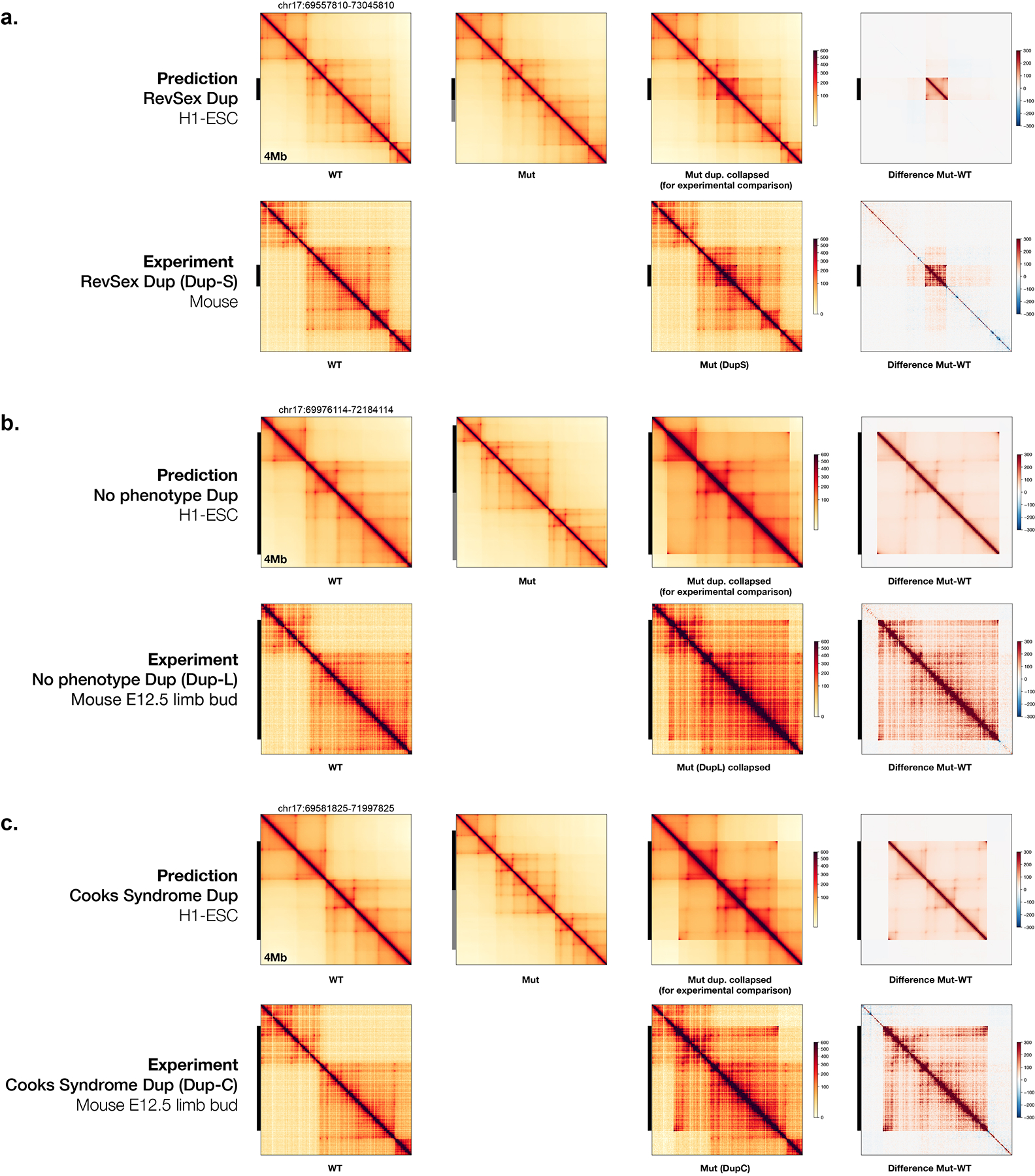
Capture Hi-C data from mouse with SVs are compared with predictions for effects of equivalent human structural variants. Predicted log fold over background at 4Mb level are scaled with the distance-expectation curve from capture Hi-C.

Extended Data Fig. 7. Multiplexed in silico mutagenesis screen results are highly correlated with single-mutation in silico mutagenesis screen results.

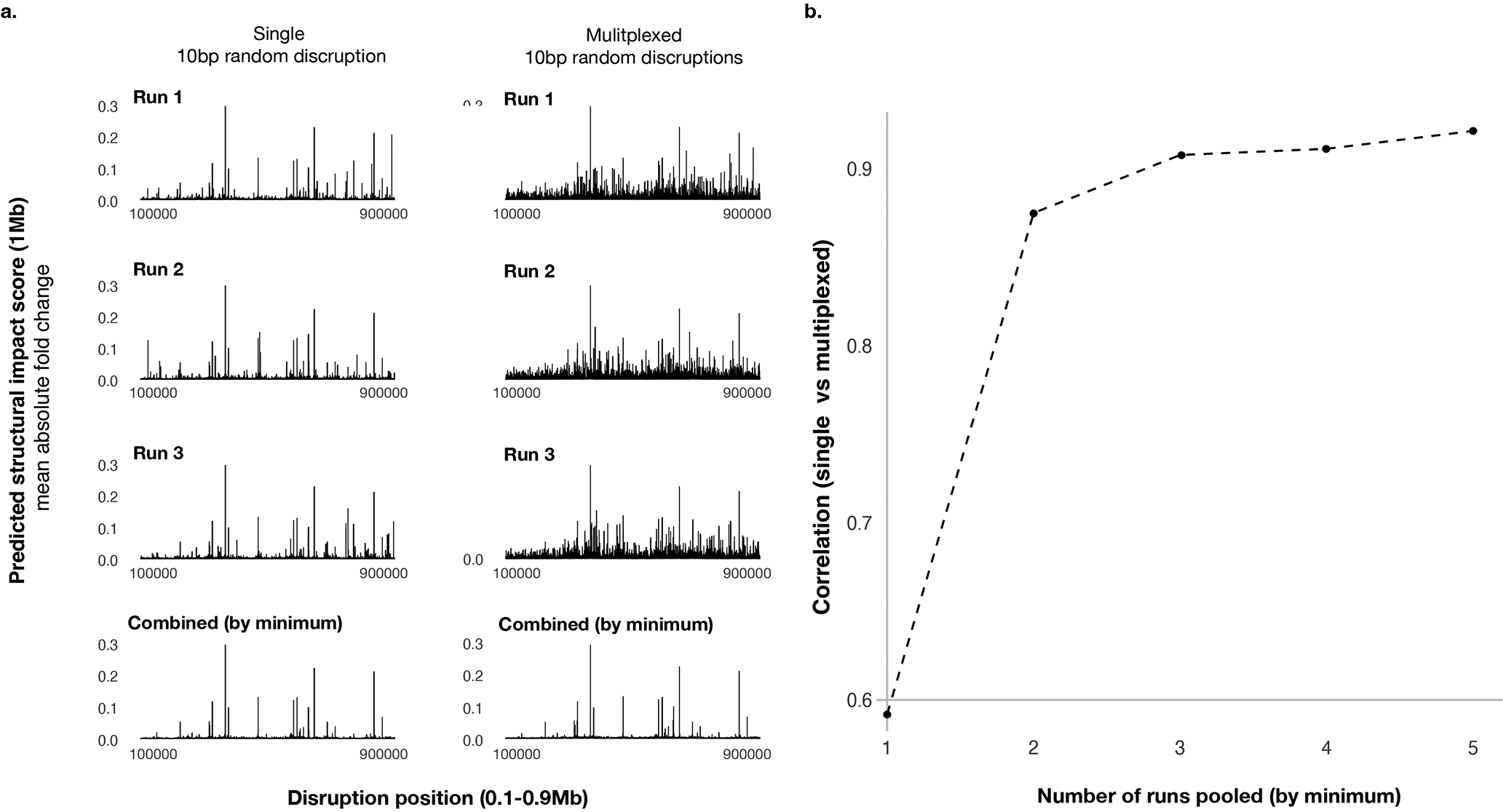
a). Predicted structural impact scores (1Mb) of single disruptions (left) and multiplexed disruptions are shown on the y-axis, with disruption positions on the x-axis. 10bp disruption sites screened cover the center 0.8Mb of the 1Mb region. The first three rows are three independent runs (for single disruption only the disrupted sequences are random across the runs, and for multiplexed disruption both the multiplex design of disruption sites and the disrupted sequences are random), and the last row shows the minimum of the three at each position. b). Relationship between the correlation of single and multiplexed disruption profiles (y-axis) and the number of runs combined (x-axis).

Extended Data Fig. 8. Visualization of virtual screen sequence activity on chromatin compartment alteration.

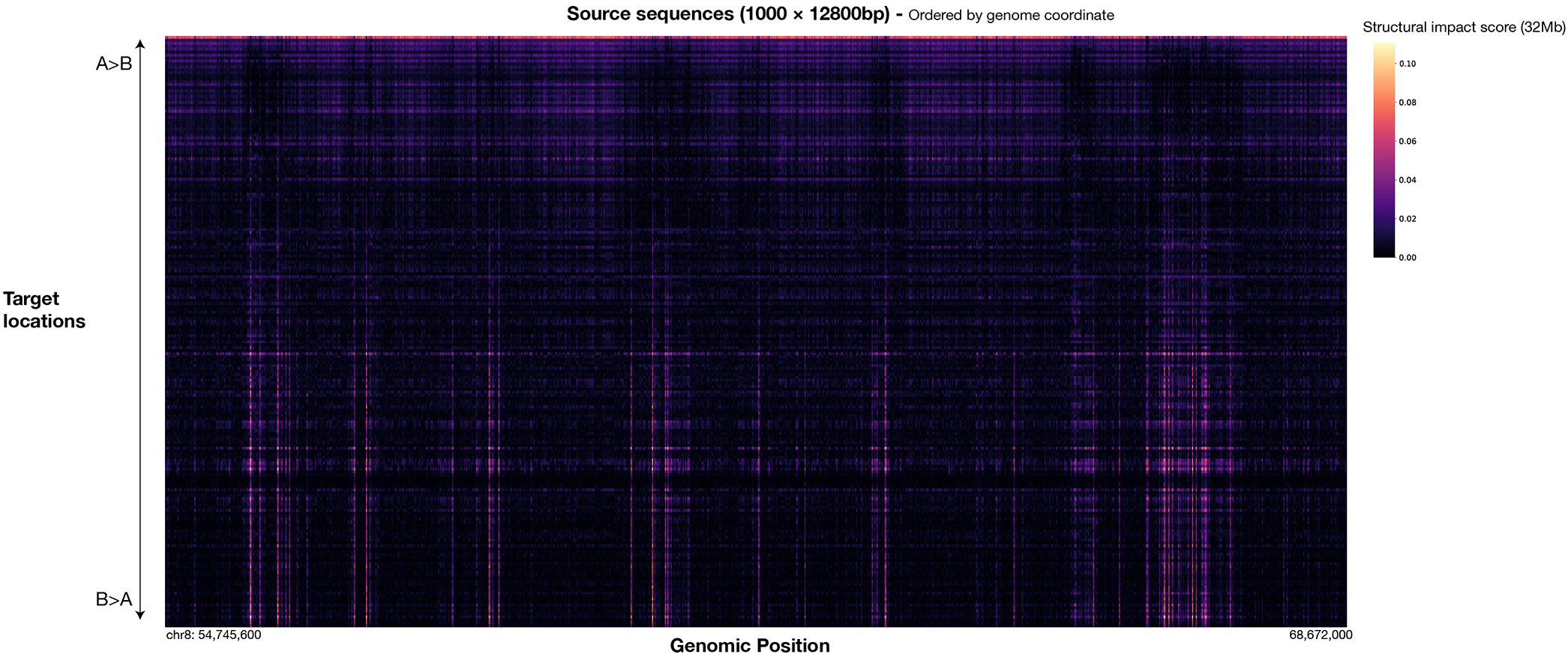
A subset of 1000 contiguous source sequences among all 27981 12800bp source sequences covering chr8, 9, and 10 are shown. Target locations are ordered by the main mode of compartment change detected at the target site (from top: A>B to bottom: B>A), which is quantified by the loading of the first principal component of the whole sequence structural impact score (32Mb) matrix.

Extended Data Fig. 9. Random sequence permutation effects on sequence compartment A and compartment B activity.

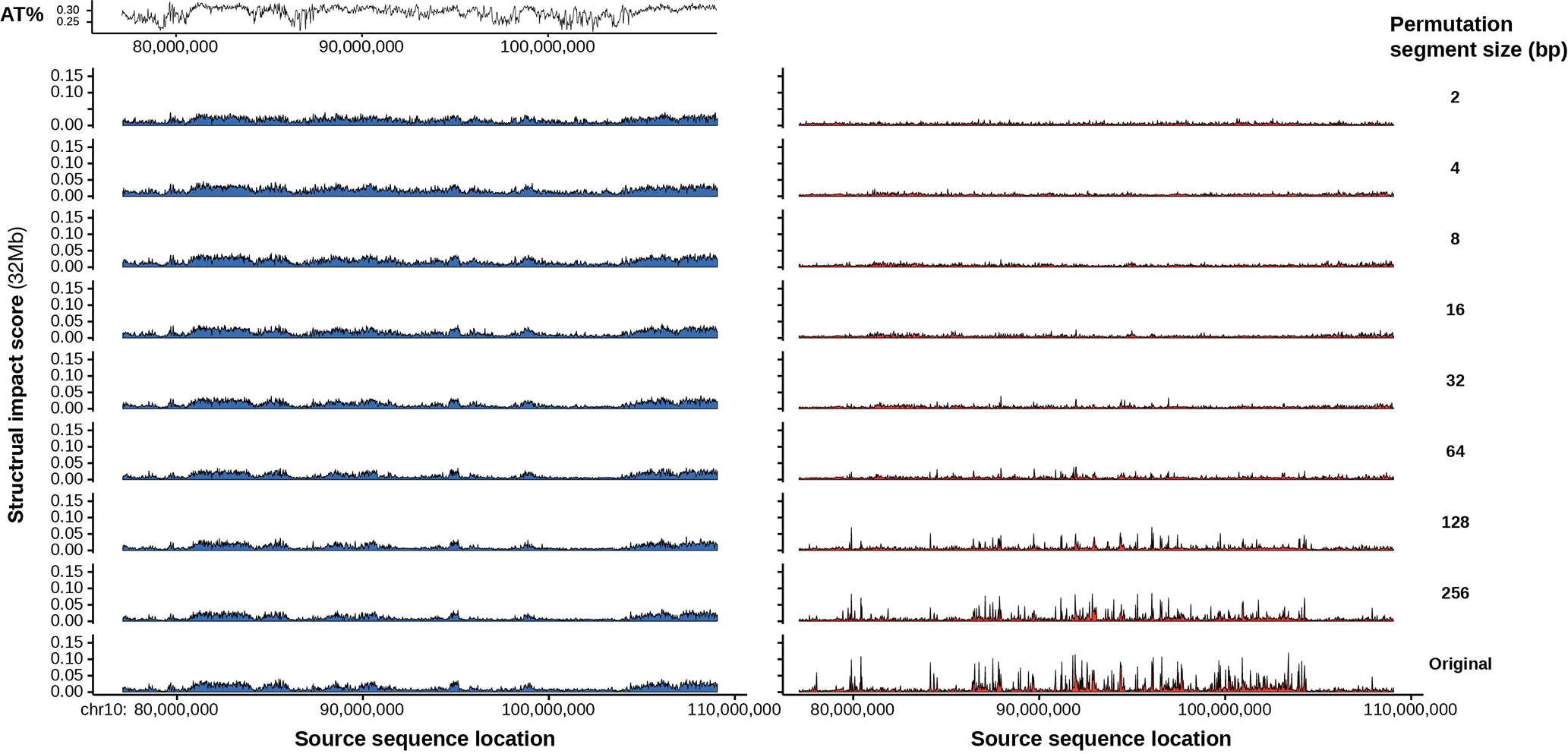
Comparison of chromatin compartment activities of 25600bp sequences permuted by different segment length (at each permutation segment length, 2bp, 4bp, …, 256bp, every 25600bp sequence is divided into segments and the segments are then randomly shuffled and concatenated). Compartment B activity is compared with sequence A/T content at the same locations.

Extended Data Fig. 10. Predicted effects of disrupting genomic regions by randomly permuting sequences.

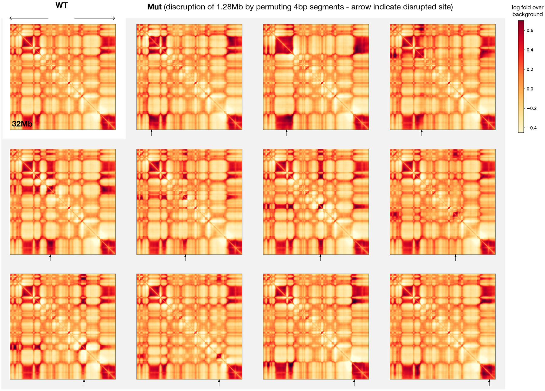
At each disruption site indicated by the arrow, 1.28Mb sequence centered at the position is permuted by 4bp segments. Permuted compartment A sequences show B compartment interaction patterns, while disrupted compartment B sequences remain to be in B compartment.

Data Availability

The GRCh38/hg38 reference genome and 3D genome datasets under 4DN accession numbers 4DNFI9GMP2J8, 4DNFI643OYP9, 4DNFILP99QJS were used for training the Orca sequence models. All coordinates in the manuscript refer to GRCh38/hg38 unless otherwise indicated. SVs experimental validation datasets were downloaded from NCBI GEO accessions GSE137372, GSE66383, GSE78109 and EBI ENA accession PRJEB5236. Data used and generated in this manuscript were also deposited into Zenodo: https://zenodo.org/record/6234936, https://zenodo.org/record/4594676, and https://zenodo.org/record/6227750.

References

- 1.Rao SSP et al. A 3D Map of the Human Genome at Kilobase Resolution Reveals Principles of Chromatin Looping. Cell 159, 1665–1680 (2014). [DOI] [PMC free article] [PubMed] [Google Scholar]
- 2.Dixon JR et al. Topological domains in mammalian genomes identified by analysis of chromatin interactions. Nature 485, 376–380 (2012). [DOI] [PMC free article] [PubMed] [Google Scholar]
- 3.Nora EP et al. Spatial partitioning of the regulatory landscape of the X-inactivation centre. Nature 485, 381–385 (2012). [DOI] [PMC free article] [PubMed] [Google Scholar]
- 4.van Steensel B & Furlong EEM The role of transcription in shaping the spatial organization of the genome. Nat. Rev. Mol. Cell Biol 20, 327–337 (2019). [DOI] [PMC free article] [PubMed] [Google Scholar]
- 5.Kosak ST et al. Subnuclear compartmentalization of immunoglobulin loci during lymphocyte development. Science 296, 158–162 (2002). [DOI] [PubMed] [Google Scholar]
- 6.Dixon JR et al. Chromatin architecture reorganization during stem cell differentiation. Nature 518, 331–336 (2015). [DOI] [PMC free article] [PubMed] [Google Scholar]
- 7.Amat R et al. Rapid reversible changes in compartments and local chromatin organization revealed by hyperosmotic shock. Genome Res. 29, 18–28 (2019). [DOI] [PMC free article] [PubMed] [Google Scholar]
- 8.Sima J et al. Identifying cis elements for spatiotemporal control of mammalian DNA replication. Cell 176, 816–830.e18 (2019). [DOI] [PMC free article] [PubMed] [Google Scholar]
- 9.Alipour E & Marko JF Self-organization of domain structures by DNA-loop-extruding enzymes. Nucleic Acids Res. 40, 11202–11212 (2012). [DOI] [PMC free article] [PubMed] [Google Scholar]
- 10.Fudenberg G, Abdennur N, Imakaev M, Goloborodko A & Mirny LA Emerging Evidence of Chromosome Folding by Loop Extrusion. Cold Spring Harb. Symp. Quant. Biol 82, 45–55 (2017). [DOI] [PMC free article] [PubMed] [Google Scholar]
- 11.Fudenberg G et al. Formation of Chromosomal Domains by Loop Extrusion. Cell Rep. 15, 2038–2049 (2016). [DOI] [PMC free article] [PubMed] [Google Scholar]
- 12.Sanborn AL et al. Chromatin extrusion explains key features of loop and domain formation in wild-type and engineered genomes. Proc. Natl. Acad. Sci. U. S. A 112, E6456–E6465 (2015). [DOI] [PMC free article] [PubMed] [Google Scholar]
- 13.Dekker J, Rippe K, Dekker M & Kleckner N Capturing Chromosome Conformation. Science 295, 1306–1311 (2002). [DOI] [PubMed] [Google Scholar]
- 14.Lieberman-Aiden E et al. Comprehensive Mapping of Long-Range Interactions Reveals Folding Principles of the Human Genome. Science 326, 289–293 (2009). [DOI] [PMC free article] [PubMed] [Google Scholar]
- 15.Krietenstein N et al. Ultrastructural Details of Mammalian Chromosome Architecture. Mol. Cell 78, 554–565.e7 (2020). [DOI] [PMC free article] [PubMed] [Google Scholar]
- 16.Zhou J & Troyanskaya OG Predicting effects of noncoding variants with deep learning–based sequence model. Nat. Methods 12, 931–934 (2015). [DOI] [PMC free article] [PubMed] [Google Scholar]
- 17.Alipanahi B, Delong A, Weirauch MT & Frey BJ Predicting the sequence specificities of DNA- and RNA-binding proteins by deep learning. Nat. Biotechnol 33, 831–838 (2015). [DOI] [PubMed] [Google Scholar]
- 18.Kelley DR, Snoek J & Rinn JL Basset: Learning the regulatory code of the accessible genome with deep convolutional neural networks. Genome Res. (2016) doi: 10.1101/gr.200535.115. [DOI] [PMC free article] [PubMed] [Google Scholar]
- 19.Zhou J et al. Deep learning sequence-based ab initio prediction of variant effects on expression and disease risk. Nat. Genet (2018) doi: 10.1038/s41588-018-0160-6. [DOI] [PMC free article] [PubMed] [Google Scholar]
- 20.Kelley DR et al. Sequential regulatory activity prediction across chromosomes with convolutional neural networks. Genome Res. 28, 739–750 (2018). [DOI] [PMC free article] [PubMed] [Google Scholar]
- 21.Chen KM, Cofer EM, Zhou J & Troyanskaya OG Selene: a PyTorch-based deep learning library for sequence data. Nat. Methods (2019) doi: 10.1038/s41592-019-0360-8. [DOI] [PMC free article] [PubMed] [Google Scholar]
- 22.Avsec Ž et al. Base-resolution models of transcription-factor binding reveal soft motif syntax. Nat. Genet 53, 354–366 (2021) [DOI] [PMC free article] [PubMed] [Google Scholar]
- 23.Fudenberg G, Kelley DR & Pollard KS Predicting 3D genome folding from DNA sequence with Akita. Nat. Methods 17, 1111–1117 (2020). [DOI] [PMC free article] [PubMed] [Google Scholar]
- 24.Schwessinger R et al. DeepC: predicting 3D genome folding using megabase-scale transfer learning. Nat. Methods 17, 1118–1124 (2020). [DOI] [PMC free article] [PubMed] [Google Scholar]
- 25.Durand NC et al. Juicebox Provides a Visualization System for Hi-C Contact Maps with Unlimited Zoom. Cell Syst 3, 99–101 (2016). [DOI] [PMC free article] [PubMed] [Google Scholar]
- 26.Abdennur N & Mirny LA Cooler: scalable storage for Hi-C data and other genomically labeled arrays. Bioinformatics 36, 311–316 (2020). [DOI] [PMC free article] [PubMed] [Google Scholar]
- 27.Chiang C et al. The impact of structural variation on human gene expression. Nat. Genet (2017) doi: 10.1038/ng.3834. [DOI] [PMC free article] [PubMed] [Google Scholar]
- 28.Zhang D et al. Alteration of genome folding via contact domain boundary insertion. Nat. Genet 52, 1076–1087 (2020). [DOI] [PMC free article] [PubMed] [Google Scholar]
- 29.Suzukawa K et al. Identification of a breakpoint cluster region 3’of the ribophorin I gene at 3q21 associated with the transcriptional activation of the EVI1 gene in acute myelogenous leukemias with inv (3)(q21q26). (1994). [PubMed]
- 30.Gröschel S et al. A single oncogenic enhancer rearrangement causes concomitant EVI1 and GATA2 deregulation in leukemia. Cell 157, 369–381 (2014). [DOI] [PubMed] [Google Scholar]
- 31.Lupiáñez DG et al. Disruptions of topological chromatin domains cause pathogenic rewiring of gene-enhancer interactions. Cell 161, 1012–1025 (2015). [DOI] [PMC free article] [PubMed] [Google Scholar]
- 32.Franke M et al. Formation of new chromatin domains determines pathogenicity of genomic duplications. Nature 538, 265–269 (2016). [DOI] [PubMed] [Google Scholar]
- 33.Croft B et al. Human sex reversal is caused by duplication or deletion of core enhancers upstream of SOX9. Nat. Commun 9, 5319 (2018). [DOI] [PMC free article] [PubMed] [Google Scholar]
- 34.Young RA Control of the embryonic stem cell state. Cell 144, 940–954 (2011). [DOI] [PMC free article] [PubMed] [Google Scholar]
- 35.Vierbuchen T et al. AP-1 Transcription Factors and the BAF Complex Mediate Signal-Dependent Enhancer Selection. Mol. Cell 68, 1067–1082.e12 (2017). [DOI] [PMC free article] [PubMed] [Google Scholar]
- 36.Rao SSP et al. Cohesin Loss Eliminates All Loop Domains. Cell (2017) doi: 10.1016/j.cell.2017.09.026. [DOI] [PMC free article] [PubMed] [Google Scholar]
- 37.Belaghzal H et al. Liquid chromatin Hi-C characterizes compartment-dependent chromatin interaction dynamics. Nat. Genet (2021) doi: 10.1038/s41588-021-00784-4. [DOI] [PMC free article] [PubMed] [Google Scholar]
- 38.Meuleman W et al. Constitutive nuclear lamina-genome interactions are highly conserved and associated with A/T-rich sequence. Genome Res. 23, 270–280 (2013). [DOI] [PMC free article] [PubMed] [Google Scholar]
- 39.Miga KH et al. Telomere-to-telomere assembly of a complete human X chromosome. Nature 585, 79–84 (2020). [DOI] [PMC free article] [PubMed] [Google Scholar]
- 40.Logsdon GA, Vollger MR & Eichler EE Long-read human genome sequencing and its applications. Nat. Rev. Genet 21, 597–614 (2020). [DOI] [PMC free article] [PubMed] [Google Scholar]
- 41.Vierstra J et al. Global reference mapping of human transcription factor footprints. Nature 583, 729–736 (2020). [DOI] [PMC free article] [PubMed] [Google Scholar]
- 42.Chen KM, Wong AK, Troyanskaya OG & Zhou J A sequence-based global map of regulatory activity for deciphering human genetics. bioRxiv (2021) doi: 10.1101/2021.07.29.454384. [DOI] [PMC free article] [PubMed] [Google Scholar]
- 43.Imakaev M et al. Iterative correction of Hi-C data reveals hallmarks of chromosome organization. Nat. Methods 9, 999–1003 (2012). [DOI] [PMC free article] [PubMed] [Google Scholar]
- 44.Izmailov P, Podoprikhin D, Garipov T, Vetrov D & Wilson AG Averaging weights leads to wider optima and better generalization. arXiv [cs.LG] (2018). [Google Scholar]
- 45.Chen T, Xu B, Zhang C & Guestrin C Training Deep Nets with Sublinear Memory Cost. arXiv [cs.LG] (2016). [Google Scholar]
- 46.Khan A et al. JASPAR 2018: update of the open-access database of transcription factor binding profiles and its web framework. Nucleic Acids Res. 46, D1284 (2018). [DOI] [PMC free article] [PubMed] [Google Scholar]
- 47.Boix CA, James BT, Park YP, Meuleman W & Kellis M Regulatory genomic circuitry of human disease loci by integrative epigenomics. Nature 590, 300–307 (2021). [DOI] [PMC free article] [PubMed] [Google Scholar]
Associated Data
This section collects any data citations, data availability statements, or supplementary materials included in this article.
Supplementary Materials
Data Availability Statement