Scan-Specific Generative Neural Network for MRI Super-Resolution Reconstruction

Abstract

The interpretation and analysis of Magnetic resonance imaging (MRI) benefit from high spatial resolution. Unfortunately, direct acquisition of high spatial resolution MRI is time-consuming and costly, which increases the potential for motion artifact, and suffers from reduced signal-to-noise ratio (SNR). Super-resolution reconstruction (SRR) is one of the most widely used methods in MRI since it allows for the trade-off between high spatial resolution, high SNR, and reduced scan times. Deep learning has emerged for improved SRR as compared to conventional methods. However, current deep learning-based SRR methods require large-scale training datasets of high-resolution images, which are practically difficult to obtain at a suitable SNR. We sought to develop a methodology that allows for dataset-free deep learning-based SRR, through which to construct images with higher spatial resolution and of higher SNR than can be practically obtained by direct Fourier encoding. We developed a dataset-free learning method that leverages a generative neural network trained for each specific scan or set of scans, which in turn, allows for SRR tailored to the individual patient. With the SRR from three short duration scans, we achieved high quality brain MRI at an isotropic spatial resolution of 0.125 cubic mm with six minutes of imaging time for T2 contrast and an average increase of 7.2 dB (34.2%) in SNR to these short duration scans. Motion compensation was achieved by aligning the three short duration scans together. We assessed our technique on simulated MRI data and clinical data acquired from 15 subjects. Extensive experimental results demonstrate that our approach achieved superior results to state-of-the-art methods, while in parallel, performed at reduced cost as scans delivered with direct high-resolution acquisition.

I. Introduction

SPATIAL resolution plays a critically important role in magnetic resonance imaging (MRI). High resolution allows for precise delineation of anatomical structures and thus enables high quality interpretation and analyses. However, high-resolution (HR) acquisition is time-consuming and costly. It is practically difficult to obtain HR images at a suitable signal-to-noise ratio (SNR) due to the potential for patient motion and other physiological noise during the long time scans [1], [2]. As a result, a trade-off between spatial resolution, SNR, and scan times is required for any MRI practices [3], [4]. Various methods have been developed to improve image quality according to this trade-off, such as parallel imaging [5], [6] and super-resolution reconstruction (SRR) [7]–[13]. Parallel imaging requires hardware supports and is platform-dependent. SRR performs in a post-acquisition manner and is thus not subject to hardware and platform limitations.

Increasing voxel size, i.e., increasing slice thickness or reducing matrix size or both, results in both reduced scan times and improved SNR given the field of view (FOV) is fixed. The underlying principle for the improvement in SNR is that the increased voxel size leads to an increase in the amount of signal received by the individual voxels. Literature has shown that SRR is unable to improve 2D in-plane or true 3D MRI due to the Fourier encoding scheme [14], [15] but is possible to enhance through-plane resolution for the acquisition of 2D slice stacks [4], [16]. Therefore, large matrix size and thick slices are commonly adopted, in pursuit of high SNR and fast imaging, resulting in images of in-plane high but through-plane low resolution. Consequently, the focus of this study is on, but not limited to, using SRR to reduce the slice thickness of 2D slice stacks acquired with short duration, to obtain images of high spatial resolution and high SNR.

SRR originated in [17] and was applied for natural images. Since SRR was introduced to MRI in [18], extensive approaches were developed for MRI SRR [7]–[9], [11], [19]–[22]. These methods are mainly classified as either model-based or learning-based SRR. Model-based SRR typically incorporates a forward model that characterizes the process of MRI acquisition, and is formulated by an inverse problem that is induced from the forward model. Since the inverse problem is in general ill-posed, priors, also known as regularization, are often leveraged to isolate the solution with desired properties from the infinitely many solutions to the HR reconstruction. State-of-the-art priors include Tikhonov cost [4], total variation (TV) [23], Huber loss [20], non-local mean method [24], and gradient guidance [25], [26]. These priors in general focus on improving the contrast and sharpness of the HR reconstruction. Learning-based SRR summarizes high frequency patterns over HR training datasets and applies these patterns to the low-resolution (LR) images being super-resolved for obtaining the HR reconstruction [27]–[31]. A common feature of the methods in this category is the requirement to present HR and LR training data, in order to be able to learn the mapping between them. However, learning by training on HR and LR data is challenging when HR inputs are difficult to obtain at suitable SNR.

Deep learning-based SRR has recently gained significant interest [32]–[40]. Techniques in this category are in general training data-oriented, rather than patient- or scan-specific, because large-scale auxiliary training datasets of HR images, which are practically difficult to obtain at satisfactory quality, are necessarily required. Although few HR MRI image datasets are publicly available for training deep neural networks, the learned SRR models may be brittle when faced with the data from a different scanner or of different intensity properties. Moreover, deep SRR models commonly contain a large number of parameters that need to be optimized during training. Once the deep model has been trained, the upsampling factor is fixed for the SRR. As the image resolution, which is determined by FOV and matrix size, may vary in different scans or with different subjects, it is impossible to apply the trained deep model to super-resolve images of arbitrarily low resolution for a desired high resolution, e.g., in applications of spatially isotropic SRR. More importantly, image contrasts may be quite different for subjects from different populations. For example, neonatal brains exhibit reversed white matter-gray matter contrast in T2-weighted scans in comparison to adult brains. Therefore, even with practically available and sufficiently large HR training datasets, current training data-oriented deep SRR models do not guarantee the success or sufficient quality of SRR for every subject in a cohort, once have completed training. These limitations suggest that it is critically important to perform SRR with a dataset-free and patient-specific deep learning technique. Such a method enables high quality SRR through powerful deep learning techniques, while in parallel, eliminates the dependence on datasets for training, and in turn, allows SRR tailored to an individual patient.

In this study, we report the development and evaluation of a dataset-free and patient-specific deep learning method for SRR. The “dataset-free” here means that the training of our deep SRR model does not require auxiliary datasets and does not even require any HR images, while the “patient-specific” or “scan-specific” means that the training leverages only the LR images that need to be super-resolved, which are all acquired from an individual patient with a short imaging time. Our technique aims at constructing images with spatial resolution higher than can be practically obtained by direct Fourier encoding while ensuring high SNR. The SRR is performed from three short duration scans with variable directions of slice selection. A deep architecture that incorporates generative and degraded neural networks is designed and learned for each individual patient on the 3D volumetric image data of low resolution. Our technique achieves high quality brain MRI at an isotropic spatial resolution of 0.125 cubic mm with six minutes of imaging time for T2 contrast and an average increase of 7.2 dB (34.2%) in SNR to these short duration scans. Experiments on both simulated and clinical data demonstrate that our SRR approach achieved superior results to state-of-the-art methods, and performed at reduced cost as scans delivered with direct HR acquisition.

II. Methods

The purpose of our approach developed and presented here is to construct images of isotropically high-resolution, at high SNR, and with short scan duration, through a deep SRR model that can be trained for an individual patient with no requirement of auxiliary datasets. A protocol that allows for short duration scans is employed to acquire LR images from an individual patient with variable directions of slice selection. The overview of our proposed deep SRR model is illustrated in Fig. 1.

Fig. 1.

Architecture of our proposed approach to scan-specific learning-based SRR. The gray boxes represent the input data, comprising an initial guess of the HR reconstruction, and n acquired LR images. All images and representations are volumetric data in the pipeline. The generative network offers an HR image based on an initial guess. The degradation networks degrade the output of the generative network to fit the LR inputs, respectively, with a mean squared error (MSE) loss. A total variation (TV) criterion is used to regularize the generative network. All losses are combined as a measure for the optimization. Only the generative network is updated during the optimization. The initial guess is obtained from an image reconstructed by a standard TV-based SRR method. The training allows for the SRR tailored to an individual patient as it is conducted on the LR images acquired from a specific patient (no auxiliary datasets of HR images are required). Once the training has been completed, the output of the generative network is taken as the HR reconstruction.

A. Acquisition strategy

The spatial resolution of an MRI image is determined by the voxel size in the acquisition. The in-plane resolution is computed from the FOV over matrix size, while the through-plane resolution is set by slice thickness. As SRR has limitations in enhancing the in-plane resolution of 2D slice stacks and true 3D scans [4], [14], [16], we fix the matrix at a large size to ensure sufficiently high in-plane resolution.

The acquisition time T of an MRI scan of 2D slice stack, delivered with a matrix size of n₁ × n₂ and n_s slices, is given by T ∝ TR · n₂ · n_s. With the fixed echo time (TE) and repetition time (TR) to keep the contrast unchanged, the option to reduce the acquisition time is to decrease the number of slices n_s, i.e., increasing the slice thickness. Also, larger thickness leads to larger voxel size, and in turn, results in higher SNR. However, the larger the thickness, the more severe the partial volume effect, and thus the more difficult the super-resolution. To this end, we acquire multiple images to facilitates SRR with an increased number of acquired slices. However, the total acquisition time is increased accordingly. Fortunately, we can employ fast imaging techniques to accelerate the scans, such as turbo spin echo (TSE) imaging. For images that yield long TR, such as T2-weighted images, the TSE technique can reduce the scan duration by N_ETL times with an echo train length of N_ETL that typically ranges from 4 to 32 in clinical practices.

We acquire multiple LR T2 TSE images with variable directions in slice selection from each subject. This method offers an effective sampling of k-space, and provides the high frequencies distributed in different directions that facilitate SRR. Although the slice selection directions and the number of the LR images can be arbitrary, orthogonal (axial, coronal, and sagittal) scans typically achieved a trade-off between acquisition time and SRR performance.

B. Acquisition model

In the spatial encoding of 2D MRI scans, a radio frequency (RF) pulse is applied in combination with a slice-select gradient to excite a slice, and then frequency- and phase-encoding steps are performed in the excited slice plane. The signals from the spatial encoding are recorded in k-space and processed to form a slice image. By repeating the above process for n_s times, a volumetric image (2D slice stack) composed of n_s slices is then acquired.

In the slice selection, a slice-select gradient is imposed along an axis perpendicular to the plane of the desired slice, leading to a linear variation of resonance frequencies in that direction. A band-pass RF pulse is simultaneously applied to excite only the desired slice containing the resonant frequencies that lie within the band. The bandwidth of the RF pulse, known as the transmitter bandwidth, denoted by BW, and the strength of the slice-select gradient G_z determine the slice thickness Δz from $\mathrm{\Delta }z=\frac{BW}{\gamma {\mathbf{G}}_z}$ with a gyromagnetic ratio γ that is a constant specific to each specific nucleus or particle. A slice profile that is related to the spectrum of the RF pulse is typically used to characterize the slice thickness in image space. For an RF pulse B₁ (t), the slice profile is given by

$${p(z)\propto \widehat{B_1}(\omega )|}_{\omega =\frac{\gamma }{2\pi }{G}_{z}z}$$ (1)

for ${\widehat{B}}_1(\omega )$ being the Fourier transform of B₁ (t).

Without loss of generality, we define the plane x-y as the imaging plane, and direction-z as the slice selection direction in the frame with axes-x, y, and z. Let m denote the magnetization density of the patient being imaged. The signal equation [42] suggests that the noise-free signal is measured from

$$s(t)=\int m(x,y,z)p(z)e^{-j2\pi (x{k}_x(t)+y{k}_y(t))}dxdydz,$$ (2)

where $k_x=\frac{\gamma }{2\pi }{\int }_0^t{G}_x(\tau )d\tau$ and $k_y=\frac{\gamma }{2\pi }{\int }_0^t{G}_y(\tau )d\tau$ with the frequency- and phase-encoding gradients G_x and G_y, respectively. This is a 2D Fourier transform of ∫ m (x, y, z) p(z) dz. Consequently, the k-th slice with a thickness of Δz mm

$$s_k={\int }_{(k-1)\text{Δ}z}^{k\text{Δ}z}m(x,y,z)p(z)dz+\epsilon$$ (3)

can be obtained from an inverse 2D Fourier transform on s(t) in combination with additive noise ε. This equation suggests that an MRI image with an arbitrary in-plane resolution and a slice thickness of Δz can be formed by convolving m (x, y, z) with the slice profile p (z) and then downsampling the convolution result in the direction of slice selection by a factor of Δz.

Let column vectors x and ${\{{\mathbf{y}}_k\}}_{k=1}^N$ denote the HR image being reconstructed and the acquired N LR images with variable directions of slice selection, respectively. The forward model that describes the imaging process is defined by

$$y_k=D_k{H}_k{T}_{k}x+{\epsilon }_k,k=1,2,\dots ,N,$$ (4)

where the matrix T_k denotes a rigid body transform in image coordinates; H_k is a circulant matrix of slice profile; D_k denotes downsampling; ε_k denotes additive noise. The details of these matrices are elaborated below.

1). Motion compensation:

Patients may move during MRI scans. We consider that they move rigidly and the motion happens only between scans as each scan duration is short. A rigid body transformation T_k is thus leveraged to represent patient motion between scans, which is composed of six degrees of freedom (three parameters for rotation, and the other three for translation). We computed the six parameters of the matrix T_k from aligning each LR image to the first images.

2). Slice encoding:

The circulant matrix H_k defines a space-invariant low-pass filter. It typically incorporates three kernels that are applied in the directions of frequency- and phase-encoding, and slice selection, respectively. Since only the through-plane resolution is enhanced, we do not consider the filtering in the directions of frequency- and phase-encoding. As discussed above, slices can be excited through a slice profile in image space by the convolution. Therefore, H_k comprises only the kernel defined by a slice profile.

An ideal slice profile is a rectangular window function with a full width of the slice thickness. It requires a sinc pulse that needs an infinite number of side lobes to uniformly and exclusively excite a discrete band of frequencies. Therefore, it is practically impossible to generate a perfectly rectangular profile. It is crucial to appropriately approximate the slice profile in SRR as the approximation directly influences the accuracy of the forward model. In general, bell-curve profiles with wider bases and narrower central peaks are leveraged, and slice thickness is measured as the full width at half maximum (FWHM) signal intensity. Gaussian profiles are widely used in MRI reconstruction and have been demonstrated to be effective in SRR [8], [20], [25], [43]–[45]. Therefore, we use the Gaussian profile with its FWHM is equal to the slice thickness in our approach. Let Δz_x denote the slice thickness of x, and Δz_k the slice thickness of y_k. The Gaussian profile incorporated in H_k is constructed with an FWHM of $\frac{\mathrm{\Delta }{z}_k}{\mathrm{\Delta }{z}_{\mathrm{x}}}$ voxels in direction-z.

3). Downsampling:

This step isolates the thick slices from the filtered thin slices of x to form the LR image y_k. As discussed above, the downsampling factor is found by $\frac{\mathrm{\Delta }{z}_k}{\mathrm{\Delta }{z}_{\mathrm{x}}}$. As this factor is not necessarily an integer, we perform the downsampling in the frequency domain by a spectrum truncation.

4). Noise:

When SNR > 3, ε_k can be considered to be additive and follows an identical Gaussian distribution [46].

C. Algorithm of super-resolution reconstruction

The basic idea of our approach is to generate an HR image using deep neural networks. The generation is restricted by the forward model in Eq. (4) based on the N acquired LR images ${\{y_k\}}_{k=1}^N$. Specifically, the HR reconstruction x is found by

$$x=f_{\mathit{\theta }}(z),\text{s.t.}{y}_k=D_k{H}_k{T}_{k}x+{\epsilon }_k,$$ (5)

with a generative function f_θ defined by a set of parameters θ based on an initial guess z. The nonlinear function f_θ is accomplished by learning a deep neural network. The initial guess z can be arbitrary due to the power of the deep network in data fitting. Since the learning for f_θ is tailored to an individual patient, only the N LR scans ${\{y_k\}}_{k=1}^N$, which are acquired from a specific patient, are used to train the deep neural network that characterizes f_θ. Random noise is incorporated in the network input in combination with z, due to the small amount of observed data in y_k, to enhance the robustness of the learning for f_θ and to prevent the learning from yielding local optima [47]. The noise, denoted by ν, follows a Gaussian distribution, of which each element is independently drawn from ν ~ $\mathcal{N}$ (0, σ²). Consequently, in combination with the Gaussian noise ε_k in the acquired LR images as discussed above, the learning for f_θ is formulated by

$$\underset{x,\mathit{\theta }}{\min }\ell (x-f_{\mathit{\theta }}(z+\mathit{\nu }))+\tau \sum _{k=1}^N\Vert y_k-D_k{H}_k{T}_{k}x{\Vert }_2^2,$$ (6)

with a loss function ℓ (·) and a weight parameter τ > 0. A similar equation can be achieved if we reformulated Eq. (5) by

$$\underset{x,\mathit{\theta }}{\min }\sum _{k=1}^N\Vert y_k-D_k{H}_k{T}_k{x}_2^2,\text{s.t.}x=f_{\mathit{\theta }}(z).$$ (7)

The above constraint is known as the deep image prior [48] in natural image processing. To increase the sharpness of the HR reconstruction, a total variation (TV) criterion [49] is imposed on the reconstruction x for image edge preservation. Consequently, the learning for f_θ is accomplished by

$$\underset{x,\mathit{\theta }}{\min }\ell (x-f_{\mathit{\theta }}(z+\mathit{\nu }))+\tau \sum _{k=1}^N\Vert y_k-D_k{H}_k{T}_{k}x{\Vert }_2^2+\mathrm{\lambda }\Vert \nabla x{\Vert }_1,$$ (8)

where λ > 0 is a weight parameter for the TV regularization and ∇x computes the image gradient of x.

The above problem can be solved by either iterative strategies that jointly optimize Eq. (8) over (x, θ) or alternate optimization techniques between x and θ. In particular, when the loss function ℓ(·) is an ℓ₂-loss, we can substitute x with f_θ:

$$\underset{\mathit{\theta }}{\min }\sum _{k=1}^N\Vert y_k-D_k{H}_k{T}_k{f}_{\mathit{\theta }}(z+\mathit{\nu }){\Vert }_2^2+\mathrm{\lambda }\Vert \nabla f_{\mathit{\theta }}(z+\mathit{\nu }){\Vert }_1,$$ (9)

This model characterizes the learning for f_θ as the following steps: 1) generate an HR image x through a nonlinear function f_θ; 2) degrade the generated image into N LR images according to the forward model; and 3) update the generation by punishing it on the residuals between the degraded images and the acquired LR images through the criterion of mean squared error in combination with a cost in edge preservation. With a learned generative function, the HR reconstruction x is consequently achieved from

$$x=f_{\mathit{\theta }}(z).$$ (10)

We implement the generative function f_θ by a deep neural network. Fig. 2 shows the design of the neural network. The initial guess z is set to an image reconstructed by a standard TV-based SRR.

Fig. 2.

Architecture of our generative neural network. The generative neural network has a structure of layers similar to 3D U-Net [41]. It comprises about 1.7M parameters distributed in the five encoder blocks, five decoder blocks, five skip blocks, and one output block. The number of channels produced by the convolution in each block is shown on the top of that block. Each skip block yields additional four channels that are concatenated with the output channels of the convolution in the respective decoder block. The filter is of size 3x3x3 voxels in each convolutional layer from the encoder and decoder blocks, and 1x1x1 voxels from the skip blocks. Reflection padding strategy is applied for all convolutions. The downsampling layers perform decimation through a stride of 2x2x2 voxels, while the upsampling layers employ trilinear interpolations with a factor of 2. The output block consists of a convolutional layer with a filter of size 1x1x1 voxels, and a sigmoid layer that normalizes the network output.

We employ N degradation networks to implement the forward model. Each degradation network contains the layers corresponding to the operations in the forward model. The filtering and downsampling are accomplished in the Fourier domain. Two additional layers are thus incorporated to provide real-to-complex discrete Fourier transform and complex-to-real inverse discrete Fourier transform, respectively. The k-th degradation network offers an output to fit an LR image y_k. Mean squared error is leveraged to quantify the fitting quality.

The TV regularization imposed on the output of the generative network is implemented by the layers that calculate image gradients in three orthogonal directions and combine them into a scalar measure by an ℓ₁-norm. The N mean squared errors in combination with the TV cost are summed up as the total loss in the learning. An Adam algorithm [50] is used to optimize the network parameters θ. The optimization takes 8K iterations for back propagation to reduce learning errors. A piecewise constant decay in learning rate is utilized, which is set at 0.01 in the first 4K iterations and then is halved every 1K iterations.

D. Assessment criteria

1). Reconstruction accuracy:

The most widely used criteria for the accuracy of image reconstruction is peak signal-to-noise ratio (PSNR) and structural similarity (SSIM) [51]. However, the two criteria are limited to using in combination with a reference image. We therefore assess our approach in terms of PSNR and SSIM on the data where ground truths are available.

2). Spatial resolution:

In MRI acquisitions, the spatial resolution is determined by the voxel size. However, in the post-processing, we can resample the voxels at arbitrary sizes. The voxel size is thus no longer an accurate measure for spatial resolution, as the resampled voxels are computed from those whose intensities may comprise a mixture of signals from multiple tissues, as shown in Eq. (2). This is also known as the partial volume effect (PVE). The spatial resolution can thus be quantified by the number of voxels suffering from PVE. The higher the spatial resolution, the fewer the voxels with PVE.

We consider three types of brain tissues in our experiments, the cerebrospinal fluid (CSF), gray matter (GM), and white matter (WM). As these tissues yield different contrasts, their voxel intensities scatter in three clusters. It has been demonstrated in [52] that the intensities of the voxels from a pure tissue follow a Gaussian distribution. Consequently, we use a Gaussian mixture model (GMM) with three components to represent the distribution of voxel intensities in an image. The GMM is obtained from a least squares data fitting to the histogram of voxel intensities. We consider the voxels are from the k-th tissue if their intensities are in the range of s_k ± δ_k for s_k and δ_k being the mean and the half FWHM of the k-th Gaussian component, respectively. Thus, the voxels outside the three ranges defined by the three tissues are from the mixture of more than one tissue, and considered as with PVE.

3). SNR:

The SNR of an image is computed from the mean signal intensity over the noise: $SNR=10{\log }_{10}\left(\frac{{\sum }_{k=1}^3{w}_k{s}_k}{v{\sum }_{k=1}^3{w}_k}\right)$, where the mean signal intensity s_k of the k-th tissue and the respective weight w_k are mean and maximum of the k-th component of the GMM obtained above, respectively, and the noise v is measured by the standard deviation of an image region from the background.

4). Contrast:

We evaluate the contrast by the metric of contrast-to-noise ratio (CNR), which is computed from the difference in the mean signal intensity between two types of tissues over the noise: $CNR=10{\log }_{10}\left(\left|s^{(1)}-s^{(2)}\right|/v\right)$.

5). Qualitative assessment:

We qualitatively evaluate the HR reconstructions and assess the capability of our approach in noise suppression. We qualitatively measure the noise by a high-pass filtered image that is obtained by 1) convolve the HR reconstruction with a Gaussian filter, and 2) subtract the Gaussian (low-pass) filtered image from the HR reconstruction.

E. Baseline methods

We employed five state-of-the-art SRR methods as the baselines, including cubic interpolation, non-local upsampling (NLU) [24], TV-regularized SRR (TV) [4], deep image prior (DIP) [48], and gradient guidance regularized SRR (GGR) [26]. As our approach utilizes the LR data only, we chose the baselines in the same category to conduct fair comparisons. Although there are many deep SRR methods in the literature, such as SR-GAN [35], [53], [54] and Variational network [30], the amount of data acquired cannot support the training for those methods. We applied the DIP method to enhance the through-plane resolution slice by slice for each LR image, and then averaged the three super-resolved images to obtain an HR reconstruction with an isotropic spatial resolution. We called our SRR approach the SSGNN (Scan-Specific Generative Neural Network) in the experiments.

F. Experimental Design

We carried out four experiments to assess our approach on both simulated and clinical data. The goal of these experiments is two-fold: 1) to demonstrate that our approach allows for the SRR tailored to an individual patient with no requirement of training datasets; and 2) to show that our approach enables fast and high quality MRI for the resolution critical use in both scientific research and clinical studies.

1). Experiment 1: Simulations on T1W and T2W data:

The objective of this experiment is to demonstrate that our approach can offer correct reconstructions while ensuring high quality. We simulated a dataset based on the structural MRI data from the Human Connectome Project (HCP) [55]. We randomly picked twenty subjects for their HR T1-weighted scans and twenty subjects for their HR T2-weighted scans. These HR scans were magnitude data and were acquired at the resolution of isotropic 0.7mm, and used as the ground truths. All simulations followed the process defined in the forward model shown in Eq. (4). We simulated three LR images from each HR image by increasing their slice thickness to 2mm in the directions-x, y, and z, respectively. Simulated motion with random translations and rotations was incorporated, which were randomly drawn from the ranges of [−10, 10] mm and [−10, 10] degrees, respectively. Random Gaussian noise, which comprised a zero mean and a standard deviation of 10% of the mean voxel intensity of the HR image, was added to each LR image. The negative intensities due to the additive noise were replaced with their absolute values. We reconstructed the HR image at the resolution of isotropic 0.7mm from the three LR images for each subject, and assessed the accuracy and quality of our reconstruction in comparison to those of the five baselines.

2). Experiment 2: Assessment on clinical T2 TSE data:

The objective of this experiment is to demonstrate that our approach can achieve images of diagnostic quality for clinical uses in six minutes of imaging time. To this end, we acquired a dataset from fifteen patients on a 3T MRI scanner. For each patient, three T2 TSE LR images were acquired in three orthogonal planes. The in-plane resolution was 0.5mm x 0.5mm and the slice thickness was 2mm. We used TR/TE=14240/95ms with an echo train length of 16, a flip angle of 160 degrees, and a pixel bandwidth of 195Hz/pixel. It took about two minutes in acquiring a T2 TSE image with this protocol. All scans were performed in accordance with the local institutional review board (IRB) protocol. We reconstructed the HR image at the resolution of isotropic 0.5mm, and assessed the reconstruction quality in terms of SNR, contrast, and spatial resolution.

3). Experiment 3: Generalization of the scan-specific training:

We aimed at investigating the generalization capability of the generative neural network trained on the scan-specific data in this experiment. Although we recommend always training on scan-specific data for the SRR, it is still helpful to investigate in what scans the scan-specific training can be generalized, and what the quality of the generalization is in those scans. The successful generalizations with satisfactory quality demonstrated that our approach can be applied to the tasks where the spatial resolution is not critical, e.g., showing a preview of the HR reconstruction before the training has been completed. In contrast, the failed generalizations demonstrated the advantages of the scan-specific training for the SRR. Consequently, we randomly selected a subject from the simulated and clinical datasets, respectively, and applied the generative neural network trained for this subject to other subjects. The generalization was achieved through Eq. (10), where the initial guess z was obtained by a standard TV method on the LR data of the testing subject. We assessed the quality of these reconstructions and analyzed the relationship between the data from these subjects. The expected outcome was that high quality generalized reconstructions were achieved for the subjects with similar image data and vice versa. In addition, as the deep generative network performs in a local manner on the image through the convolution, we investigated similarities between the training and testing data in the generalization mode through the local correlation [56], also known as local self-similarity [57]. Our expectation was that high quality generalized reconstructions were obtained when high local correlations between the training and testing data were observed and vice versa.

4). Experiment 4: Ablation studies and algorithm analyses:

The objective of this experiment is to investigate the contributions and of each module in our approach to the SRR. As shown in Eq. (9), our SRR model incorporates three important modules that need to investigate: the generative network f_θ the Gaussian noise ν added to the initial guess z, and the TV regularization. The contribution of the generative network to the SRR was demonstrated by the performance gap between SSGNN to TV. We visualized the intermediate reconstructions from different decoder layers to analyze how the generative network performed. We assessed our SRR approach by training the generative network on different numbers of LR scans, in order to analyze how the number of LR scans affected the training and in turn the SRR results. We also investigated how the slice thickness affected the performance of our SRR approach by evaluating the reconstruction accuracy over the LR data with different thicknesses. The Gaussian noise ν ~ $\mathcal{N}$ (0, σ²) is controlled by the parameter σ, while the TV regularization yields the weight parameter λ. The module was removed when we set the respective parameter to zero. We investigated how different values of the parameters influenced the SRR. We evaluated the reconstruction accuracy with the parameters on ten T1W and ten T2W scans that we randomly picked from the HCP dataset.

III. Results

We implemented our SRR in PyTorch [58] and ran it on an NVIDIA Titan RTX GPU. It took about six hours to reconstruct an image of size 384³ voxels. We reported the quantitative results by box and whisker plots [59], [60]. In each box, the central line indicated the median, and the bottom and top edges of the box indicated the 25th and 75th percentiles, respectively. The whiskers extended to the most extreme data points.

A. Experiment 1: Simulations on T1W and T2W data

Fig. 3 shows the results of our approach and the five baselines in terms of PSNR and SSIM on the HCP dataset. Our approach, SSGNN, achieved a PSNR of 38.11±2.11dB and an SSIM of 97.0±0.005 on average. The results show that SSGNN offered the most accurate reconstructions of both T1W and T2W images on this dataset, and in particular, outperformed the second best method, GGR, with a large margin in SSIM.

Fig. 3.

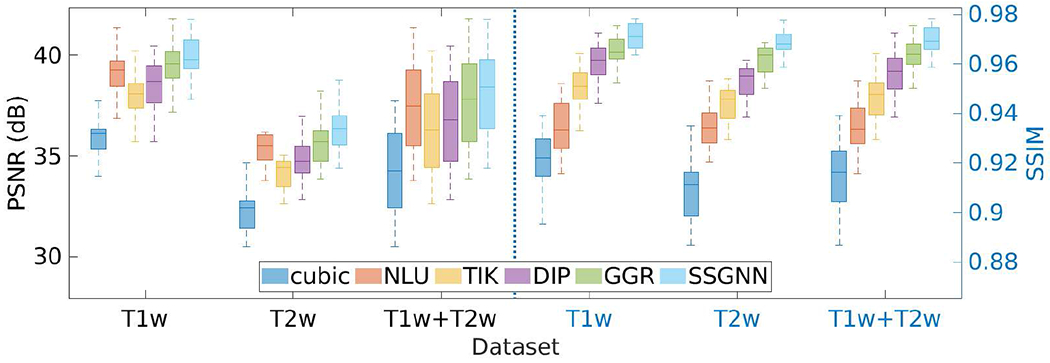
Results of our approach (SSGNN) and the five baseline methods in terms of PSNR and SSIM on the HCP dataset. SSGNN generated the most accurate results on this dataset.

Fig. 4 shows the results of our approach and the five baselines in terms of SNR, CNR, and PVE on the HCP dataset. Our approach achieved an average SNR of 23.8±2.32dB, and considerably outperformed the baselines in terms of SNR and CNR. The percentage of voxels with PVE in our reconstructed images was 10.4%±3.5% on average. The results show that SSGNN offered the highest spatial resolution on this dataset.

Fig. 4.

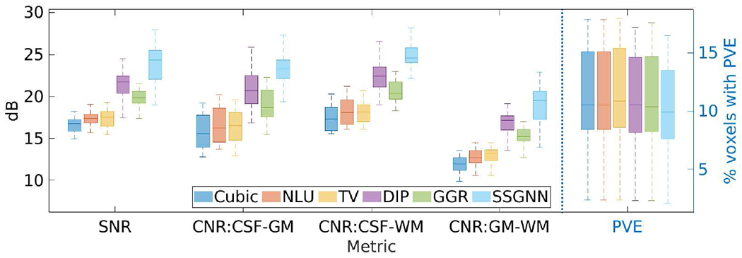
Results of our approach (SSGNN) and the five baselines in terms of SNR, CNR, and partial volume effect (PVE) on the HCP dataset. SSGNN considerably outperformed the baselines in terms of SNR and CNR, and offered the highest spatial resolution in terms of PVE on this dataset.

Fig. 5(a) shows the estimation of PVE. The blue curve with markers shows the distribution of voxel intensities of a selected image region that contained CSF, GM, and WM. A GMM with three components was leveraged to fit the distribution of voxel intensities, as depicted by the solid line. The three components of the GMM, represented from left to right the WM, GM, and CSF, respectively, are plotted by the dashed lines. Fig. 5(b) shows the converging process of our approach in terms of mean squared error and PSNR with 8K iterations. The results show that SSGNN converged after 2K iterations in this example.

Fig. 5.

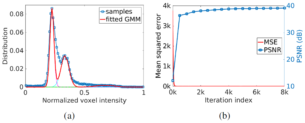
Results in example images from the HCP dataset. (a) Estimation of partial volume effect. The blue curve with markers shows the distribution of voxel intensities of a selected image region that contained CSF, GM, and WM. A Gaussian mixture model (GMM) with three components was leveraged to fit the distribution of voxel intensities, as depicted by the solid line. The three components of the GMM, represented from left to right the WM, GM, and CSF respectively, are plotted by the dashed lines. (b) Converging process of our approach in terms of mean squared error and PSNR with 8,000 iterations.

Fig. 6 shows the qualitative results of our approach and the five baselines on the HCP dataset in comparison to the images from direct HR acquisitions. The results in the top line show that our approach, SSGNN, performed the best in noise suppression, and considerably reduced the noise compared to the direct HR acquisitions. The middle line shows that SSGNN offered the best qualitative performance in the image details and noise suppression, particularly in the cerebellum as highlighted in the images. The results in the bottom line show that SSGNN yielded the best image quality, and in particular, SSGNN offered finer anatomical structures of the cerebellum at a lower noise level, and in turn, achieved superior reconstructions to the direct HR acquisitions as well as the five baselines.

Fig. 6.

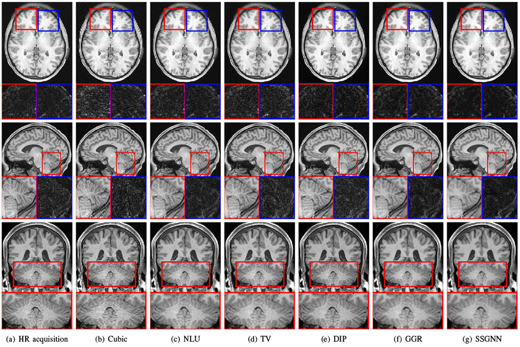
Slices from the direct HR acquisitions and HR reconstructions on the HCP dataset. The top line shows the comparisons in the axial slices and noise levels. The noise detected from the highlighted patches is shown below the axial slices. The results show that our approach (SSGNN) performed the best in noise suppression, and considerably reduced the noise compared to the HR acquisition. The middle line shows the comparisons in the sagittal slices and their noise levels. SSGNN offered the best qualitative results according to the image details and noise suppression, particularly in the cerebellum as highlighted in the images. The bottom line shows the results in the coronal plane. SSGNN yielded the best image quality. In particular, SSGNN offered finer anatomical structures of the cerebellum at a lower noise level, and in turn, achieved superior reconstructions to the direct HR acquisitions as well as the five baselines.

B. Experiment 2: Assessment on clinical T2 TSE data

Fig. 7 shows the results of SSGNN and the five baselines in terms of SNR, CNR, and PVE on the clinical dataset. SSGNN considerably outperformed the five baselines according to SNR and CNR. It yielded an average SNR of 28.1±3.3dB, which was 11.6% (2.9dB) higher than obtained by the second best method, GGR, and 34.2% (7.2dB) higher than obtained by Cubic. The percentage of voxels with PVE achieved by SSGNN was 9.3%±5.9% on average, which was the lowest among those obtained by the six methods. Therefore, SSGNN offered the highest spatial resolution on this dataset.

Fig. 7.

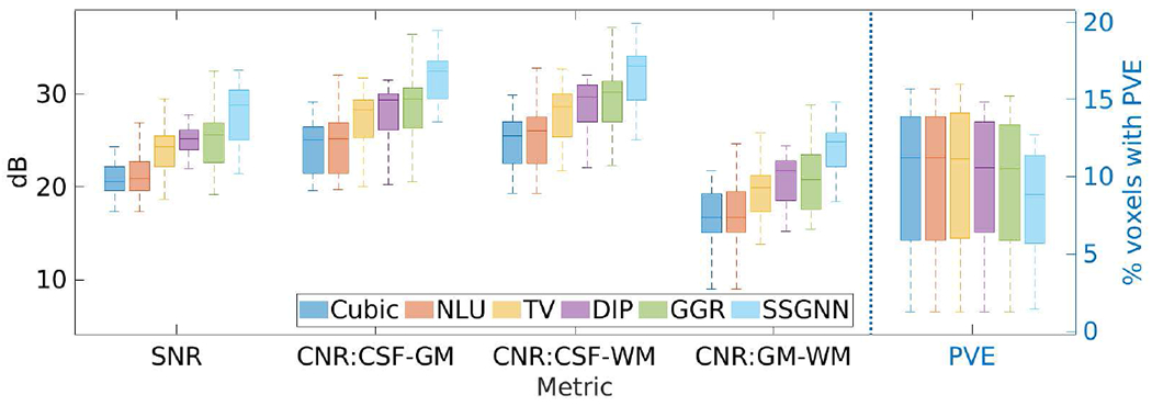
Results of our approach (SSGNN) and the five baselines in terms of SNR, CNR, and partial volume effect (PVE) on the clinical dataset. SSGNN considerably outperformed the five baselines according to SNR and CNR, and offered the highest spatial resolution in terms of PVE on this dataset.

Fig. 8 shows the voxels suffering from PVE in the images reconstructed by the five baselines and our approach from a representative subject on the clinical dataset. SSGNN offered the lowest number of voxels with PVE, leading to the highest spatial resolution in the reconstructed HR image.

Fig. 8.

Voxels suffering from partial volume effect (PVE) in the images reconstructed by the five baselines and our approach (SSGNN) from a representative subject on the clinical dataset. SSGNN offered the lowest number of voxels with PVE, leading to the highest spatial resolution in the reconstructed HR image.

Figs. 9–11 show the qualitative results of our approach and the five baselines on the clinical dataset. Fig. 9 shows that SSGNN achieved the best result according to the image details and sharpness. As highlighted in these slices, SSGNN offered finer anatomical structures of the vermis and cerebrocerebellum than the five baselines. As shown in Fig. 10, SSGNN generated the best reconstruction according to the image details. In particular, SSGNN offered much clearer and sharper image edges in the cerebral cortex than the five baselines. The results in Fig. 11 show that SSGNN achieved the sharpest reconstruction and yielded the most precise anatomical structures of the cerebrum, particularly in the frontal lobe as highlighted in the images.

Fig. 9.

Qualitative results of our approach (SSGNN) and the five baselines on the clinical dataset. SSGNN performed the best according to the image details and sharpness. As highlighted in these slices, SSGNN offered finer anatomical structures of the vermis and cerebrocerebellum than the five baselines.

Fig. 11.

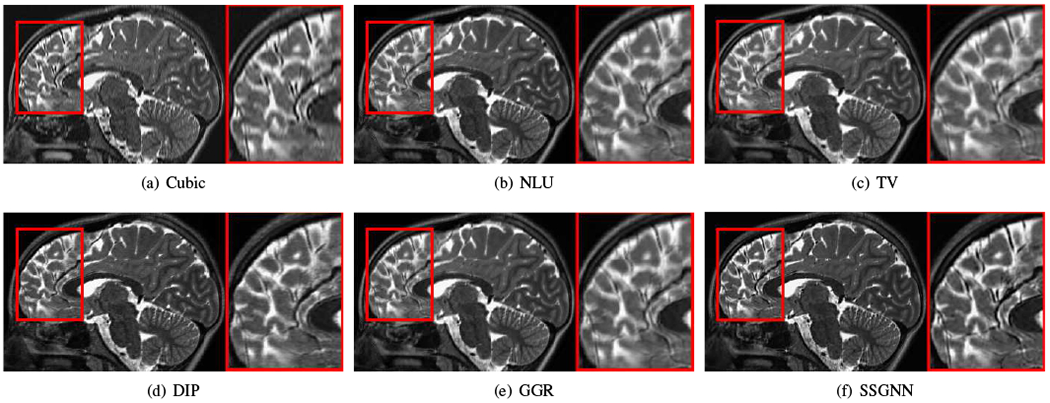
Qualitative results of our approach (SSGNN) and the five baseline methods on the clinical dataset. The results show that SSGNN generated the sharpest reconstruction and offered the most precise anatomical structures of the cerebrum, particularly in the frontal lobe as highlighted in the images.

Fig. 10.

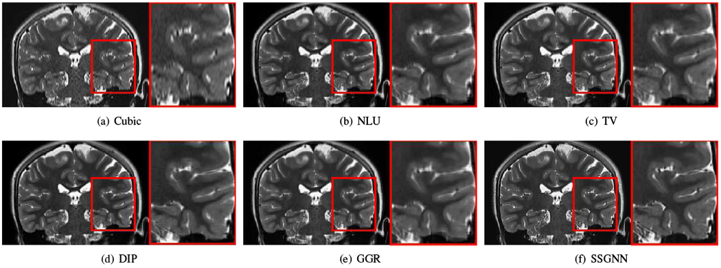
Qualitative results of our approach (SSGNN) and the five baseline methods on the clinical dataset. The results show that SSGNN generated the best reconstruction according to the image details. In particular, SSGNN offered much clearer and sharper image edges in the cerebral cortex than the five baselines.

Fig. 12 shows the reconstructions over iterations obtained by our SRR approach from a neonate. The anatomies, such as the hippocampus, were clearly delineated after 1000 iterations, while in the following iterations, our SRR algorithm fine-tuned the reconstruction in the contrasts and SNR.

Fig. 12.

Reconstructions over iterations obtained by our approach from a neonate. The anatomies, e.g., the hippocampus, were clearly delineated after 1000 iterations, while in the following iterations, our SRR algorithm fine-tuned the reconstruction in the contrasts and SNR.

C. Experiment 3: Generalization of the scan-specific training

Fig. 13 shows the generalization analyses on the HCP dataset. The results show that the generalized generative network, denoted by SSGNN-Gen, offered superior reconstructions to the initial guess obtained from the TV method but inferior results to SSGNN trained on the scan-specific data in terms of PSNR and SSIM. Also, SSGNN-Gen generated better results on the T2w scans than on the T1w scans, as the standard deviation of the distributions of the T2w intensity is smaller than that of the T1w intensity, as shown in Fig. 13(a).

Fig. 13.

Generalization analyses on the HCP dataset. (a) Means and standard deviations of distributions of voxel intensity on all T1w and T2w ground truths. (b) Accuracy of the generalized reconstructions in terms of PSNR and SSIM. The results show that the generalized generative network (SSGNN-Gen) offered superior reconstructions to the initial guess obtained from TV but inferior results to SSGNN trained on the scan-specific data. SSGNN-Gen generated better results on the T2w scans than on the T1w scans as the standard deviation of the distributions of the T2w intensity is smaller than that of the T1w intensity.

Fig. 14 shows three HR images reconstructed by our SRR approach (SSGNN) for three representative subjects on the clinical dataset. Subjects 1 and 2 were young children at a similar age, so their voxel intensity distributions were similar as well, as shown in Fig. 14(d). Subject 3 was a newborn and had reverse gray matter-white matter contrasts as compared to the other two subjects, resulting in a big difference in the voxel intensity distribution from Subjects 1 and 2. These results can also be interpreted by the difference in the local correlation. We extracted the image patches of size 3x3x3 voxels from all subjects and computed the correlations between each patch from Subjects 1 and 2, and from Subjects 1 and 3. We showed the distribution of the maximum local correlation of each patch, as plotted in Fig. 14(e). The results show that the local correlations between Subjects 1 and 2 were much higher than between Subjects 1 and 3, leading to better generalization from Subject 1 to Subject 2 than to Subject 3.

Fig. 14.

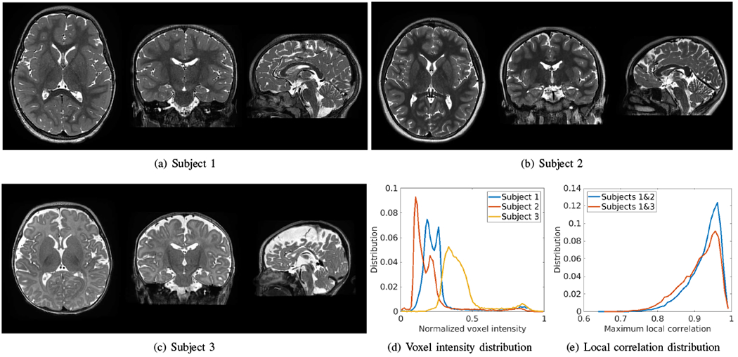
HR images reconstructed by our SRR approach (SSGNN) for three representative subjects on the clinical dataset. Subjects 1 and 2 were young children at the similar age, so their voxel intensity distributions were similar as well, as plotted in (d). Subject 3 was a newborn and had reverse gray matter-white matter contrasts as compared to the other two subjects, resulting in a big difference in the voxel intensity distribution from Subjects 1 and 2. These results can also be interpreted by the difference in the local correlation, as plotted in (e), where the local correlations between Subjects 1 and 2 were much higher than between Subjects 1 and 3.

Fig. 15 shows the generalized reconstructions for Subjects 2 and 3. The generative network was trained for Subject 1 and applied to Subjects 2 and 3. The HR images reconstructed by SSGNN, as shown in Fig. 14, were used as the gold standards. The results show that the generalization for Subject 2 was successful and led to small errors, while failed for Subject 3 with big errors due to the big difference in intensity distributions between Subjects 1 and 3.

Fig. 15.

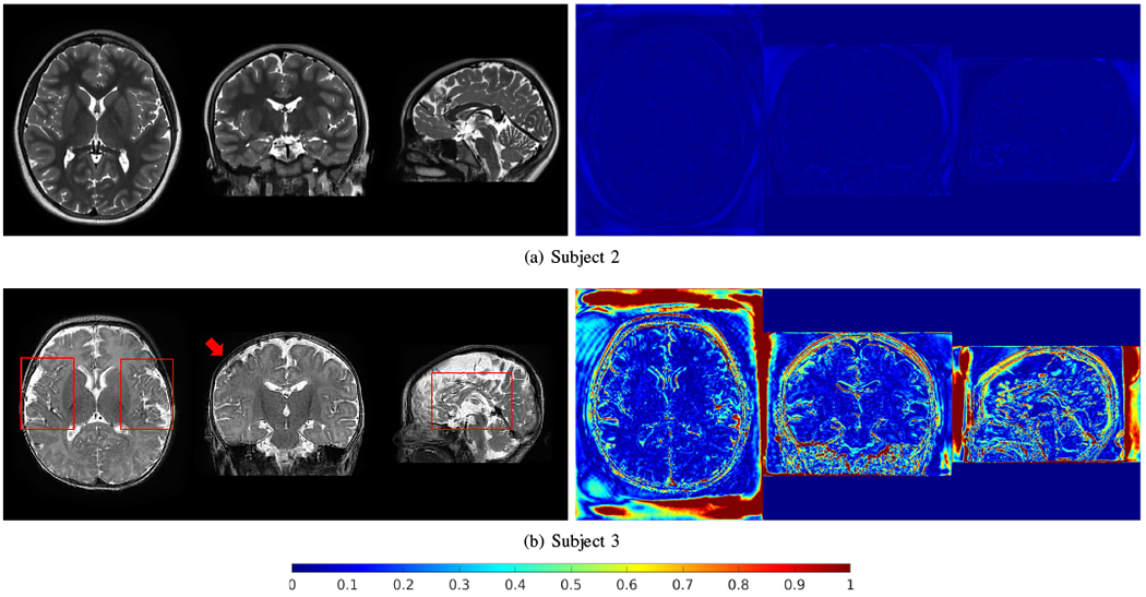
Generalized reconstructions for Subjects 2 and 3. The generative network was trained for Subject 1 and applied to Subjects 2 and 3. The HR images reconstructed by SSGNN, as shown in Fig. 14, were used as the gold standards. The generalization for Subject 2 was successful and led to small errors (right column), while failed for Subject 3 with big errors due to the big difference in intensity distributions between Subjects 1 and 3.

D. Experiment 4: Ablation studies and algorithm analyses

Fig. 16 visualizes the representative intermediate reconstructions in different decoder layers. The visualizations show that the decoder captured the image details in different scales with different layers.

Fig. 16.

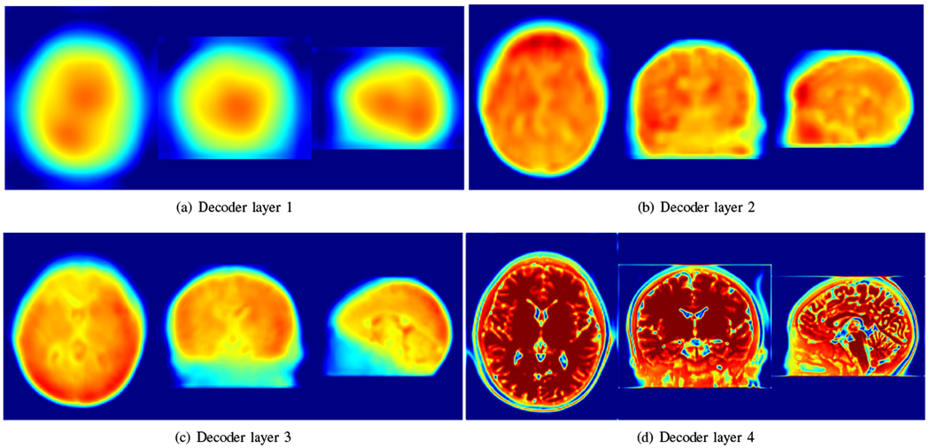
Visualization of representative intermediate reconstructions in different decoder layers. The visualizations show that the decoder captured the image details in different scales with different layers.

Fig. 17 shows the results of the investigation on the number of LR scans incorporated in our approach on the HCP dataset in terms of PSNR and SSIM. The results show that our approach performed better as more LR scans were leveraged.

Fig. 17.

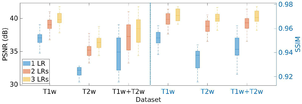
Results of the investigation on the number of LR scans incorporated in our approach on the HCP dataset in terms of PSNR and SSIM. The results show that our approach performed better as more LR scans were leveraged.

Fig. 18 shows the results of the investigation on the slice thickness of the LR scans incorporated in our approach on the HCP dataset in terms of PSNR and SSIM. The results show that the performance of our SRR approach performed better with thinner slices.

Fig. 18.

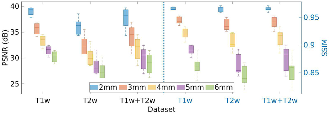
Results of the investigation on the slice thickness of LR scans incorporated in our approach on the HCP dataset in terms of PSNR and SSIM.

Fig. 19 shows the results of the investigation on the standard deviation σ of the Gaussian noise ν added to the initial guess z, as shown in Eq. (8), on the HCP dataset in terms of PSNR and SSIM. We set the parameter σ at different values in the range of [0, 0.1], and performed the SRR at each value. The results show that our approach achieved the highest accuracy when setting σ at 0.05. The PSNR and SSIM were 37.3±2.2 dB and 0.96±0.005, respectively, at this value of σ. The results in the case of σ = 0 show that adding noise to the network input led to an increase in the accuracy of our SRR approach by 5% in PSNR and by 4% in SSIM, respectively.

Fig. 19.

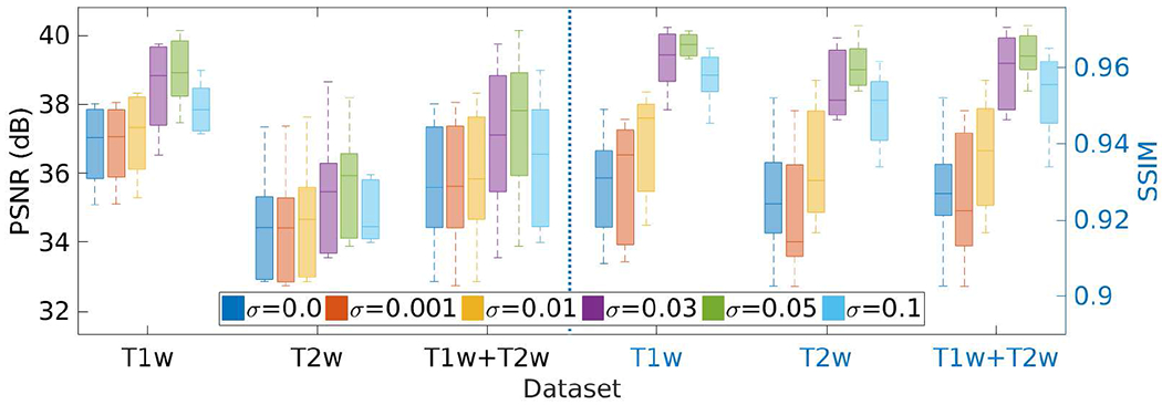
Results of the investigation on the standard deviation σ of the Gaussian noise ν added to the network input z on the HCP dataset in terms of PSNR and SSIM. SSGNN achieved the best results when setting σ at 0.05.

Fig. 20 shows the results of the investigation on the weight parameter λ of the TV regularization on the HCP dataset in terms of PSNR and SSIM. We set the parameter λ at different values in the range of [0, 0.5], and performed the SRR at each value. The results show that our approach achieved the highest accuracy when setting λ at 0.01. The PSNR and SSIM were respectively 37.7±2.2dB and 0.97±0.006 on average. The results in the case of λ = 0 show that the TV regularization improved the accuracy of our SRR approach by 2% in PSNR and by 1% in SSIM, respectively.

Fig. 20.

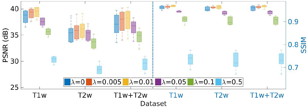
Results of the investigation on the weight parameter λ of the TV regularization on the HCP dataset in terms of PSNR and SSIM. SSGNN generated the best results when setting λ at 0.01.

IV. Discussion

We have developed a technique that allows for auxiliary dataset-free deep learning-based SRR. We have demonstrated that our technique enables the deep SRR model tailored to an individual patient. We have applied this technique to perform scan-specific SRR for high quality MRI.

A. Reconstruction quality

We have shown in the simulation experiment that our approach correctly converged, as shown in Fig. 5(b), for solving our SRR problem presented in Eq. (8). We have also shown in Fig. 3 that our approach generated correct reconstructions, and substantially improved the reconstruction accuracy in terms of PSNR and SSIM, as compared to the five baselines. These results have demonstrated that our technique ensures the reliability and applicability of our SRR approach for use in scientific research studies and clinical practices.

The maximum voxel intensity in the T1W images from the HCP dataset was much higher than in the T2W images. As PSNR is proportional to the maximum voxel intensity, the PSNR in T1W images were higher than in T2W images, as shown in Fig. 3. Thus, the difference in PSNR between T1W and T2W images in the simulation experiment did not indicate the performance bias of our approach in different sequences.

We have shown that our approach considerably improved the SNR and CNR of the reconstructed HR images in comparison to the five baselines, as reported in Figs. 4 and 7. This is attributed to the denoising by the encoder-decoder network [48] (the generative network) in combination with the image deconvolution (inversion of the forward model) in our design, as shown in Eq. (8). GGR and TV also led to improved SNR and CNR as they incorporated image deconvolution as well.

We have shown that our approach achieved the highest spatial resolution in terms of PVE on both the simulated and clinical datasets, as shown in Figs. 4 and 7. When the resolution shifted from 0.7mm on the HCP dataset to 0.5mm on the clinical dataset, as expected, the estimated number of voxels with PVE in our SRR decreased from 10.4% to 9.3% on average. As shown in Fig. 8, the PVE incurred in those voxels from the boundaries of different types of tissues. These results have demonstrated that our approach allows for high spatial resolution for delineating the details of anatomical structures.

Our approach enhances the through-plane resolution in the image space, i.e., it processes magnitude data for the reconstruction. The major advantage of using image space instead of raw data is that it allows for a general SRR beyond imaging platforms and protocols, as it is flexible, convenient, and does not require hardware information like coil sensitivities. The downside is thus that the phase data is not available in the reconstruction. As the phase data in general contains information about magnetic field inhomogeneities, our approach is not suitable in those applications such as the characterization of susceptibility-induced distortions.

B. Acquisition strategy

We have shown that how the number and thickness of LR scans affected our SRR approach, respectively, as shown in Figs. 17 and 18. The results show that our approach performed better with more LR scans and thinner slices. These results were consistent with those of the majority of SRR techniques, i.e., SRR algorithms benefit from an increased number of observations and small downsampling factors. However, acquiring an increased number of LR scans increases scan time, while acquiring thin slices lengthens scan times and reduces SNR. It has been shown in [1] that the pediatric patients hold their heads still for six minutes on average in brain MRI exams. Our fast acquisition protocol ensured acquiring an LR T2 TSE image with a thickness of 2 mm in two minutes. We thus acquired three LR images for a patient with six minutes of imaging time. Therefore, our acquisition strategy allows for high SNR in a single LR scan, while mitigating motion during the scans. Consequently, this is a trade-off between the quality of SRR and scan time. The experimental results have demonstrated the efficacy of our acquisition strategy.

C. Acquisition time reduction

We have shown that our approach acquired a T2 TSE image at the resolution of 0.5mm x 0.5mm x 2mm in two minutes. It is considerably fast to obtain an image with T2 contrast at the resolution of isotropic 0.5mm in six minutes of total imaging time. As a comparison, in six minutes of imaging time, we can only acquire a 3D T2 SPACE image at the resolution of isotropic 1mm on our 3T scanner. Acquiring that same data at the resolution of isotropic 0.5mm can be carried out, but acquires about 8 times more data, and thus requires an extended acquisition time. In addition, the SNR is reduced by a factor of 8 as each voxel shifts from 1 cubic mm to 0.5³ cubic mm. In order to obtain a satisfactory SNR, averaging over multiple HR data is required, leading to further extended acquisition time. Consequently, our approach offered a fast imaging solution to high-resolution brain MRI at a high SNR, which substantially reduced the in-scanner acquisition time.

D. A deconvolution perspective

The generative network offers an HR image as the reconstruction, while the degradation networks degrade the HR reconstruction to fit the LR scans. The optimal reconstruction is achieved when the residual between the degraded images and the LR scans is minimized. The optimization process is essentially a super-resolution strategy that comprises upsampling and deconvolution.

Our super-resolution model is presented in Eq. (9). The optimization is accomplished by a numerical algorithm based on a gradient descent strategy. Without loss of generality, a standard gradient descent algorithm can be leveraged to search in the solution space for optimal reconstruction. The derivative of the objective function J in Eq. (9) is found by

$$\frac{\partial J}{\partial \mathit{\theta }}=\frac{\partial J}{\partial f_{\mathit{\theta }}}\cdot \frac{\partial f_{\mathit{\theta }}}{\partial \mathit{\theta }}.$$ (11)

For simplicity, we consider the data fidelity (the ℓ₂-norm term) only. Consequently, we have

$$\frac{\partial J}{\partial \mathit{\theta }}=\sum _{k=1}^N{T}_k^T{H}_k^T{D}_k^T(D_k{H}_k{T}_k{f}_{\mathit{\theta }}-y_k)\cdot \frac{\partial f_{\mathit{\theta }}}{\partial \mathit{\theta }}.$$ (12)

The above equation shows the update rule for θ in the numerical algorithm. The HR reconstruction f_θ is estimated with θ at the current iteration, transformed onto each LR scan space by T_k, blurred by H_k, and undersampled by D_k. The degraded image is then compared to the LR scan y_k and then the residual is upsampled by $D_k^T$, deconvolved by ${\mathbf{H}}_k^T$, and transformed back onto the HR image space by $T_k^T$. These results are summed up and then propagated into the network parameter space for a step of update in θ. Therefore, the optimization process mainly relies on upsampling and deconvolution for the super-resolution reconstruction, which is a typical strategy to solve the super-resolution model [4], [24], [25]. The superiority of our approach is accomplished by the dynamically learned regularization delivered by the deep neural networks. The generative network yields the HR reconstruction with the constraints imposed by its encoding-decoding scheme, while the degradation networks offer the upsampling and deconvolution framework and enforce the data fidelity.

E. High-resolution generation

The primitive SRR problem is severely ill-posed as it tries to estimate a large number of unknowns (voxel intensities of the HR reconstruction) from a limited number of observations (all voxels of the acquired LR images). Priors, also known as regularization, are typically incorporated to pick the desired solution (HR reconstruction) from the infinitely many feasible solutions (HR reconstructions that can be derived from the observations). The priors define certain criteria that measure the desired properties in the candidates of HR reconstructions. A candidate that matches these criteria the best is then selected as the HR reconstruction.

The forward model defines an inverse problem for the SRR in our approach, which is also severely ill-posed as ${\mathrm{\sum }}_{k=1}^N$ #y_k ≪ #x with # counting the voxels. We use a nonlinear function implemented by training a deep neural network to generate the HR reconstruction according to the rules defined by the forward model. The neural network comprises a number of encoder and decoder layers where the knowledge about the HR generation with the underlying degradation process is dynamically embedded based on the acquired LR images. A successful application of such knowledge in natural image processing has been known as deep image prior [48]. By training the deep SRR model over the LR images, the scheme combining the generative neural network and its degradation counterparts defines an implicit criterion that distinguishes the HR reconstruction represented the best by the networks from the infinitely many candidates. Such an implicit criterion is delivered by the network structure through parameterization. As shown in Eq. (7), the regularization is applied by the nonlinear function f_θ that enforces the mapping from the code vector z to the HR reconstruction x. It suggests that the generative network searches the solution space by adjusting the parameters of its convolutional filters, in order to explain/represent the HR reconstruction x the best. Such an explanation/representation establishes the implicit criterion according to the parameterization as well as the data fidelity. Eqs. (11) and (12) have shown that the network embeds the knowledge captured by the parameters θ into the HR reconstruction. These parameters are optimized during the training according to the code vector z and, the LR images y_k, and the forward model for each individual learning process. Therefore, the criterion for regularization varies in each reconstruction. We address the regularization as a dynamically learned prior with an implicit criterion, as the prior in fact does not have an explicit form that we can describe in a mathematical or structural manner. This conclusion has also been demonstrated in [48].

The representation-based regularization is often used in super-resolution methods, such as dictionary learning-based representation [29] and sparse convolutional representation [61]. The techniques in this category typically impose task-specific, handcrafted constraints on the feature maps that represent the HR reconstruction. Similarly, in our approach, the HR reconstruction is deeply represented by the deep generative neural network. A set of encoder layers address the feature maps based on a code vector, and then a set of decoder layers restore the HR reconstruction over the learned feature maps. This process is fully unsupervised and adaptive over the input data. There is no explicit constraint on the representations, but the deep representation of the HR reconstruction promises an implicit regularization via the deep network structure. It has been shown in [48] that such an implicit criterion delivered by the deep neural network with an “hourglass” structure offers high impedance to noise and low impedance to signal. The performance gap between SSGNN and TV has shown the contribution of the dynamically learned prior to the quality of the SRR.

As an example, we have shown in Fig. 16 that the decoder captured the image details in different scales with different layers. All details were integrated into the output of the generative network. The integration implicitly delivered the prior that the HR reconstruction was the one out of infinitely many candidates, which was represented the best by the generative network, or equivalently, approximated the most accurately by the nonlinear function f_θ.

F. Scan-specific learning v.s. training data-oriented learning

Our scan-specific learning for SRR relies on the LR data only that is acquired from a specific patient, in contrast to the training data-oriented learning that requires large-scale auxiliary datasets of HR images. Therefore, our technique allows for the SRR tailored to an individual patient, resulting in superior HR reconstructions in comparison to training data-oriented techniques. Although we recommend always using scan-specific learning with our approach, we have still investigated how our SRR performed when working in the mode of training data-oriented learning. The underlying scheme that the generalization mode works is the local similarity between the training and testing data. The generative network offers the HR reconstruction through convolutions that are performed over the local patches. So the generative network captures the local features in the reconstruction. When the local patches in the training data are sufficiently similar to those in the testing data, the generalization on the testing data will be successful. It has been shown in the literature that there is such a similarity residing in the local patches of MRI images, referred to as self-similarity [57], and also known as the local correlation [56]. Consequently, the training captures the statistical properties that are desired to generalize the learned model.

We trained our SRR model on the LR data from a randomly picked subject, and then applied this trained model to perform our SRR (to generate HR reconstructions through f_θ) for other subjects. The results reported in Figs. 13–15 have shown that our SRR model trained on the scan-specific data can be generalized to perform in a training data-oriented manner when the distributions of voxel intensity yielded small differences. These results can also be interpreted by the difference in the local correlation, as plotted in Fig. 14(e). The success of the generalization suggests that our deep model correctly captured the image prior so that the prior can be generalized in the reconstructions of other images. This enables applications of our technique in the tasks, e.g., showing a preview of the HR reconstruction before the scan-specific training has been completed. Also, the generalization failed for the data with quite different distributions of voxel intensity and led to incorrect reconstructions, as shown in Fig. 15(b). These failures demonstrated the necessity and advantages of our scan-specific learning technique.

G. A data fitting viewpoint

The majority of learning methods for deep convolutional networks learn data statistics/inherent properties over large-scale training data sets. Those learned statistics can then be applied for inference tasks over unseen data. Different from the common paradigm used in those methods, our approach aims at fitting a generative network to a single (set of) LR scan(s). As discussed above, the network weights play a role of parameterization to constrain the reconstructed HR image. The image statistics, required to exploit the information lost in the degradation process, are captured through the parameterization of the generative network in combination with the constraint delivered by the forward model. Therefore, our SRR can be regarded as a conditional image generation problem, where the only information required to solve the SRR is the input LR scans and the designed structure of the generative neural network. As the network weights are initialized randomly, the only prior provided is the network structure. As shown in Eq. (9), our purpose is to fit the network weights θ to the input LR scans ${\{{\mathbf{y}}_k\}}_{k=1}^N$ according to the degradation defined in the forward model. Once the fitting has been maximally accomplished, the image statistics are captured by the generative network and the information lost revealed through these statistics is integrated into the HR reconstruction. Consequently, the ultimate goal of network training in our approach is to fit the network to the input data, rather than to summarize priors over a large number of training samples. So our approach does not require auxiliary training sets. On the other hand, we have demonstrated that using the “Noise2noise” learning strategy [47] further enhanced the SRR performance of the learned generative network by adding Gaussian noise to the network input (refer to Fig. 19). Instead of performing in the scan-specific learning mode, we have also shown that the fitted network worked in a generalization mode for those images that have similar patterns of voxel intensity distributions. However, we cannot ensure the fitted network for a set of images still fits the other set of images. Therefore, we recommend always using our approach in the scan-specific learning mode.

H. Contributions of major modules

We have investigated the major modules of our SRR approach. The performance gap between our approach (SSGNN) and TV depicted the contributions of the generative neural network with the scan-specific learning, by referring to Eqs. (8) and (9). It has shown that our generative network led to the improvement in SNR by 36.3% (6.33dB) and 17.1% (4.1dB), and in spatial resolution by 10.3% and 17.8% on the HCP and clinical datasets, respectively. The investigations on the parameters σ and λ have shown that, on the HCP dataset, the Gaussian noise added to the initial guess resulted in an increase in PSNR by 4.7% and SIIM by 3.9% due to the promoted robustness of the training, and that the TV regularization increased the PSNR by 2.1% and SSIM by 0.8% due to the edge preservation constraint.

Although TV regularization has been one of the most widely used method in MRI reconstruction, it has been shown that it may lead to staircase artifacts in the reconstructed image its piecewise constant form [62]–[64]. Our approach incorporates a TV regularization in combination with a deep image prior, as shown in Eq. (9), so the staircase artifacts were not observed in our HR reconstructions. We included the TV method as a baseline to demonstrate the efficacy of the prior dynamically learned by our deep neural networks. Considering the improvement by the TV regularization was relatively minor, we recommend removing it from the learning presented in Eq. (9) in pursuit of the rapid converge of the optimization at the cost of losing accuracy a little bit if reconstruction time is limited.

I. Reconstruction time

It took about six hours to reconstruct an image with 384³ voxels by using our SRR approach. Therefore, our approach is suitable in research imaging and those clinical applications where the reconstruction time is not critical. As our approach does not make assumptions on the quality of LR scans, the reconstruction quality can be predicted according to the quality of LR scans. The radiologists or technologists can immediately decide if they complete the scans or need to reacquire some data, e.g., due to patient motion, by qualitatively assessing the quality of the acquired LR scans with the real-time feedback provided by the scanner. If the reconstruction time is critical in some tasks, we recommend reducing the iterations in the optimization of Eq. (9). As shown in Figs. 5 and 12, the quality of the reconstructions was acceptable after 1000 iterations. So the SRR can be accomplished in 45 minutes with satisfactory quality. Although the reconstruction can be obtained in a few seconds when performing our SRR in the manner of training data-oriented learning on the data with similar intensity distributions, we recommend always using the scan-specific learning mode to perform the SRR.

J. Related reconstruction techniques

A related category of techniques is 2D regularized parallel imaging [65]–[68]. These techniques allow for substantially reduced acquisition time, as compared to conventional imaging methods and 3D acquisition such as T2 SPACE mentioned above. Unfortunately, 2D parallel imaging acceleration undersamples the data and reduces the measured signal and the measured SNR. The widely used pseudo-inverse image space solution and convolution k-space solution to exploiting coil sensitivity profiles to estimate unmeasured data both amplify measurement noise in a spatially varying manner. This is known as g-factor artifact (geometry factor artifact). Regularization reduces the variability of the output voxels given change in the measured signal, but it does so in a manner that causes a bias in the signal intensities. The reconstructed image thus has the wrong intensity value, instead of zero mean noise perturbations around the correct value. The regularization can only provide a good image when the prior model used for regularization makes assumptions that are true of the anatomy being imaged.

We take advantage of undersampling which allows us to form three undersampled scans with reduced acquisition time. We encode the HR k-space data with three rapid undersampled observations of the HR k-space data convolved with a spatially oriented low-pass filter (being oriented axial, coronal, and sagittal). Our approach is performed in a deconvolution manner, with which the reconstruction benefits from the prior dynamically learned through the scheme combining the generative neural network and its degradation counterparts. It has demonstrated that such a learned prior is particularly effective in the suppression of noise amplification [48], as well as demonstrated in our experiments reported in Figs. 4 and 7. Consequently, our approach allows for high SNR in a short acquisition time, while 2D regularized parallel imaging has been still struggling in improving SNR in the reconstructed images. Furthermore, our generative neural network architecture can also be used as a prior in parallel imaging reconstruction by replacing the forward model (degradation networks) with the corresponding data consistency term, e.g., the sensitivity encoding model [5].

K. Conclusions

In conclusion, we have developed a deep neural network-based technique that enables scan-specific learning for SRR with no requirement of training datasets. With this technique, we have demonstrated a methodology that allows for constructing high quality images at the resolution of isotropic 0.5mm with dramatically reduced imaging time (with only 6 minutes of imaging time), as compared to direct HR acquisition. Extensive experimental results have demonstrated that our approach offered fast and diagnostic quality MRI for the resolution critical use in both scientific research and clinical studies.

References

- [1].Afacan O, Erem B, Roby DP, Roth N, Roth A, Prabhu SP, and Warfield SK, “Evaluation of motion and its effect on brain magnetic resonance image quality in children,” Pediatric Radiology, vol. 46, no. 12, pp. 1728–1735, 2016. [DOI] [PMC free article] [PubMed] [Google Scholar]
- [2].Sui Y, Afacan O, Gholipour A, and Warfield SK, “SLIMM: Slice Localization Integrated MRI monitoring,” NeuroImage, vol. 223, no. 117280, pp. 1–16, 2020. [DOI] [PMC free article] [PubMed] [Google Scholar]
- [3].Brown RW, Cheng Y-CN, Haacke EM, Thompson MR, and Venkatesan R, Magnetic resonance imaging: Physical principles and sequence design, 2nd Edition. Wiley, 2014. [Google Scholar]
- [4].Plenge E, Poot DHJ, Bernsen M, Kotek G, Houston G, Wielopolski P, van der Weerd L, Niessen WJ, and Meijering E, “Super-resolution methods in MRI: Can they improve the trade-off between resolution, signal-to-noise ratio, and acquisition time?” Magnetic Resonance in Medicine, vol. 68, pp. 1983–1993, 2012. [DOI] [PubMed] [Google Scholar]
- [5].Pruessmann KP, Weiger M, Scheidegger MB, and Boesiger P, “SENSE: Sensitivity encoding for fast MRI,” Magnetic Resonance in Medicine, vol. 42, pp. 952–962, 1999. [PubMed] [Google Scholar]
- [6].Griswold MA, Jakob PM, Heidemann RM, Nittka M, Jellus V, Wang J, Kiefer B, and Haase A, “Generalized autocalibrating partially parallel acquisitions (GRAPPA),” Magnetic Resonance in Medicine, vol. 47, no. 6, pp. 1202–1210, 2002. [DOI] [PubMed] [Google Scholar]
- [7].Greenspan H, “Super-Resolution in Medical Imaging,” The Computer Journal, vol. 52, no. 1, pp. 43–63, 2009. [Google Scholar]
- [8].Gholipour A, Estroff JA, Sahin M, Prabhu SP, and Warfield SK, “Maximum a posteriori estimation of isotropic high-resolution volumetric mri from orthogonal thick-slice scans,” in Medical Image Computing and Computer-Assisted Intervention (MICCAI), 2010, pp. 109–116. [DOI] [PMC free article] [PubMed] [Google Scholar]
- [9].Van Reeth E, Tham IW, Tan CH, and Poh CL, “Super-resolution in magnetic resonance imaging: A review,” Concepts in Magnetic Resonance, vol. 40, no. 6, pp. 306–325, 2012. [Google Scholar]
- [10].Scherrer B, Gholipour A, and Warfield SK, “Super-resolution reconstruction to increase the spatial resolution of diffusion weighted images from orthogonal anisotropic acquisitions,” Medical Image Analysis, vol. 16, no. 7, pp. 1465–1476, 2012. [DOI] [PMC free article] [PubMed] [Google Scholar]
- [11].Gholipour A, Afacan O, Aganj I, Scherrer B, Prabhu SP, Sahin M, and Warfield SK, “Super-resolution reconstruction in frequency, image, and wavelet domains to reduce through-plane partial voluming in MRI,” Medical Physics, vol. 42, no. 12, pp. 6919–6932, 2015. [DOI] [PMC free article] [PubMed] [Google Scholar]
- [12].Dalca AV, Bouman KL, Freeman WT, Rost NS, Sabuncu MR, and Golland P, “Medical Image Imputation From Image Collections,” IEEE Transactions on Medical Imaging, vol. 38, no. 2, pp. 504–514, 2019. [DOI] [PMC free article] [PubMed] [Google Scholar]
- [13].Sui Y, Afacan O, Gholipour A, and Warfield SK, “Fast and High-Resolution Neonatal Brain MRI Through Super-Resolution Reconstruction From Acquisitions With Variable Slice Selection Direction,” Frontiers in Neuroscience, vol. 15, no. 636268, pp. 1–15, 2021. [DOI] [PMC free article] [PubMed] [Google Scholar]
- [14].Scheffler K, “Superresolution in MRI?” Magnetic Resonance in Medicine, vol. 48, p. 408, 2002. [DOI] [PubMed] [Google Scholar]
- [15].Peled S and Yeshurun Y, “Super-resolution in MRI – Perhaps sometimes,” Magnetic Resonance in Medicine, vol. 48, p. 409, 2002. [Google Scholar]
- [16].Greenspan H, Oz G, Kiryati N, and Peled S, “MRI inter-slice reconstruction using super-resolution,” Magnetic Resonance Imaging, vol. 20, no. 5, pp. 437–446, 2002. [DOI] [PubMed] [Google Scholar]
- [17].Tsai R and Huang T, “Multi-frame image restoration and registration,” in Advances in computer vision and image processing, 1984. [Google Scholar]
- [18].Fiat D, “Method of enhancing an mri signal,” US Patent 6,294,914, 2001.
- [19].Shilling RZ, Robbie TQ, Bailloeul T, Mewes K, Mersereau RM, and Brummer ME, “A Super-Resolution Framework for 3-D High-Resolution and High-Contrast Imaging Using 2-D Multislice MRI,” IEEE Transactions on Medical Imaging, vol. 28, no. 5, pp. 633–644, 2009. [DOI] [PubMed] [Google Scholar]
- [20].Gholipour A, Estroff JA, and Warfield SK, “Robust super-resolution volume reconstruction from slice acquisitions: application to fetal brain MRI,” IEEE Transactions on Medical Imaging, vol. 29, no. 10, pp. 1739–1758, 2010. [DOI] [PMC free article] [PubMed] [Google Scholar]
- [21].Scherrer B, Afacan O, Taquet M, Prabhu SP, Gholipour A, and Warfield SK, “Accelerated High Spatial Resolution Diffusion-Weighted Imaging,” in International Conference on Information Processing in Medical Imaging (IPMI), 2015. [DOI] [PMC free article] [PubMed] [Google Scholar]
- [22].Aganj I, Lenglet C, Yacoub E, Sapiro G, and Harel N, “A 3D wavelet fusion approach for the reconstruction of isotropic-resolution MR images from orthogonal anisotropic-resolution scans,” Magnetic Resonance in Medicine, vol. 67, no. 4, pp. 1167–1172, 2012. [DOI] [PMC free article] [PubMed] [Google Scholar]
- [23].Tourbier S, Bresson X, Hagmann P, Thiran J, Meuli R, and Cuadra M, “An efficient total variation algorithm for super-resolution in fetal brain MRI with adaptive regularization,” Neuroimage, vol. 118, pp. 584–597, 2015. [DOI] [PubMed] [Google Scholar]
- [24].Manjón JV, Coupé P, Buades A, Fonov VS, Collins DL, and Robles M, “Non-local MRI upsampling,” Medical Image Analysis, vol. 14, no. 6, pp. 784–792, 2010. [DOI] [PubMed] [Google Scholar]
- [25].Sui Y, Afacan O, Gholipour A, and Warfield SK, “Isotropic mri super-resolution reconstruction with multi-scale gradient field prior,” in Medical Image Computing and Computer-Assisted Intervention (MICCAI), 2019. [DOI] [PMC free article] [PubMed] [Google Scholar]
- [26].Sui Y, Afacan O, Jaimes C, Gholipour A, and Warfield S, “Gradient-guided isotropic mri reconstruction from anisotropic acquisitions,” IEEE Transactions on Computational Imaging, pp. 1–1, 2021. [DOI] [PMC free article] [PubMed] [Google Scholar]
- [27].Ravishankar S and Bresler Y, “Mr image reconstruction from highly undersampled k-space data by dictionary learning,” IEEE Transactions on Medical Imaging, vol. 30, pp. 1028–1041, 2011. [DOI] [PubMed] [Google Scholar]
- [28].Jia Y, He Z, Gholipour A, and Warfield SK, “Single anisotropic 3d mr image upsampling via overcomplete dictionary trained from in-plane high resolution slices,” IEEE Journal of Biomedical Health Informatics, vol. 20, no. 6, pp. 1552–1561, 2016. [DOI] [PMC free article] [PubMed] [Google Scholar]
- [29].Jia Y, Gholipour A, He Z, and Warfield SK, “A new sparse representation framework for reconstruction of an isotropic high spatial resolution mr volume from orthogonal anisotropic resolution scans,” IEEE Transactions on Medical Imaging, vol. 36, no. 5, pp. 1182–1193, 2017. [DOI] [PMC free article] [PubMed] [Google Scholar]
- [30].Hammernik K, Klatzer T, Kobler E, Recht M, Sodickson D, Pock T, and Knoll F, “Learning a variational network for reconstruction of accelerated mri data,” Magnetic Resonance in Medicine, vol. 79, 2018. [DOI] [PMC free article] [PubMed] [Google Scholar]
- [31].Akçakaya M, Moeller S, Weingärtner S, and Ugurbil K, “Scan-specific robust artificial-neural-networks for k-space interpolation (raki) reconstruction: Database-free deep learning for fast imaging,” Magnetic Resonance in Medicine, vol. 81, pp. 439–453, 2019. [DOI] [PMC free article] [PubMed] [Google Scholar]
- [32].Pham C, Ducournau A, Fablet R, and Rousseau F, “Brain mri superresolution using deep 3d convolutional networks,” in International Symposium on Biomedical Imaging, 2017, pp. 197–200. [Google Scholar]
- [33].Chen Y, Xie Y, Zhou Z, Shi F, Christodoulou AG, and Li D, “Brain mri super resolution using 3d deep densely connected neural networks,” in International Symposium on Biomedical Imaging, 2018, pp. 739–742. [Google Scholar]
- [34].Chaudhari A, Fang Z, Kogan F, Wood J, Stevens K, Gibbons E, Lee J, Gold G, and Hargreaves B, “Super-resolution musculoskeletal MRI using deep learning,” Magnetic Resonance in Medicine, vol. 80, no. 5, pp. 2139–2154, 2018. [DOI] [PMC free article] [PubMed] [Google Scholar]
- [35].Chen Y, Shi F, Christodoulou AG, Xie Y, Zhou Z, and Li D, “Efficient and accurate mri super-resolution using a generative adversarial network and 3d multi-level densely connected network,” in Medical Image Computing and Computer-Assisted Intervention (MICCAI), 2018. [Google Scholar]
- [36].Zhao X, Zhang Y, Zhang T, and Zou X, “Channel splitting network for single MR image super-resolution,” IEEE Transactions on Image Processing, vol. 28, no. 11, pp. 5649–5662, 2019. [DOI] [PubMed] [Google Scholar]
- [37].Wang J, Chen Y, Wu Y, Shi J, and Gee J, “Enhanced generative adversarial network for 3d brain mri super-resolution,” in IEEE Winter Conference on Applications of Computer Vision, 2020, pp. 3627–3636. [Google Scholar]
- [38].Xue X, Wang Y, Li J, Jiao Z, Ren Z, and Gao X, “Progressive sub-band residual-learning network for MR image super-resolution,” IEEE Journal of Biomedical Health Informatics, vol. 24, no. 2, pp. 377–386, 2020. [DOI] [PubMed] [Google Scholar]
- [39].Cherukuri V, Guo T, Schiff SJ, and Monga V, “Deep MR brain image super-resolution using spatio-structural priors,” IEEE Transactions on Image Processing, vol. 29, pp. 1368–1383, 2020. [DOI] [PMC free article] [PubMed] [Google Scholar]
- [40].Sui Y, Afacan O, Gholipour A, and Warfield SK, “Learning a gradient guidance for spatially isotropic mri super-resolution reconstruction,” in Medical Image Computing and Computer-Assisted Intervention (MICCAI), 2020. [DOI] [PMC free article] [PubMed] [Google Scholar]
- [41].Çiçek Ö, Abdulkadir A, Lienkamp S, Brox T, and Ronneberger O, “3D U-Net: Learning dense volumetric segmentation from sparse annotation,” in Medical Image Computing and Computer-Assisted Intervention (MICCAI), 2016. [Google Scholar]
- [42].Bloch F, Hansen W, and Packard M, “The nuclear induction experiment,” Physical Review, vol. 70, no. 7, pp. 474–485, 1946. [Google Scholar]
- [43].Rousseau F, Glenn O, Iordanova B, Rodríguez-Carranza C, Vigneron D, Barkovich A, and Studholme C, “A novel approach to high resolution fetal brain mr imaging,” Medical image computing and computer-assisted intervention : MICCAI … International Conference on Medical Image Computing and Computer-Assisted Intervention, vol. 8 Pt 1, pp. 548–55, 2005. [DOI] [PubMed] [Google Scholar]
- [44].Jiang S, Xue H, Glover A, Rutherford M, Rueckert D, and Hajnal J, “Mri of moving subjects using multislice snapshot images with volume reconstruction (svr): Application to fetal, neonatal, and adult brain studies,” IEEE Transactions on Medical Imaging, vol. 26, pp. 967–980, 2007. [DOI] [PubMed] [Google Scholar]
- [45].Murgasova M, Quaghebeur G, Rutherford M, Hajnal J, and Schnabel JA, “Reconstruction of fetal brain mri with intensity matching and complete outlier removal,” Medical Image Analysis, vol. 16, pp. 1550–1564, 2012. [DOI] [PMC free article] [PubMed] [Google Scholar]
- [46].Gudbjartsson H and Patz S, “The Rician Distribution of Noisy MRI Data,” Magnetic Resonance in Medicine, vol. 34, pp. 910–914, 1995. [DOI] [PMC free article] [PubMed] [Google Scholar]
- [47].Lehtinen J, Munkberg J, Hasselgren J, Laine S, Karras T, Aittala M, and Aila T, “Noise2noise: Learning image restoration without clean data,” in Proceedings of the 35th International Conference on Machine Learning (ICML), vol. 80, 2018, pp. 2971–2980. [Google Scholar]
- [48].Ulyanov D, Vedaldi A, and Lempitsky V, “Deep image prior,” 2018 IEEE/CVF Conference on Computer Vision and Pattern Recognition (CVPR), pp. 9446–9454, 2018. [Google Scholar]
- [49].Rudin L, Osher S, and Fatemi E, “Nonlinear total variation based noise removal algorithms,” Physica D: Nonlinear Phenomena, vol. 60, pp. 259–268, 1992. [Google Scholar]
- [50].Kingma DP and Ba J, “Adam: A method for stochastic optimization,” in International Conference on Learning Representations (ICLR), 2015. [Google Scholar]
- [51].Wang Z, Bovik AC, Sheikh HR, and Simoncelli EP, “Image quality assessment: From error measurement to structural similarity,” IEEE Transactions on Image Processing, vol. 13, no. 1, pp. 600–612, 2004. [DOI] [PubMed] [Google Scholar]
- [52].Laidlaw D, Fleischer K, and Barr AH, “Partial-volume Bayesian classification of material mixtures in MR volume data using voxel histograms,” IEEE Transactions on Medical Imaging, vol. 17, pp. 74–86, 1998. [DOI] [PubMed] [Google Scholar]
- [53].Ledig C, Theis L, Huszár F, Caballero J, Aitken A, Tejani A, Totz J, Wang Z, and Shi W, “Photo-realistic single image super-resolution using a generative adversarial network,” in IEEE Conference on Computer Vision and Pattern Recognition (CVPR), 2017, pp. 105–114. [Google Scholar]
- [54].Sanchez I and Vilaplana V, “Brain mri super-resolution using 3d generative adversarial networks,” in Medical Imaging with Deep Learning, 2018. [Google Scholar]
- [55].Essen D, Smith S, Barch D, Behrens TEJ, Yacoub E, and Ugurbil K, “The wu-minn human connectome project: An overview,” NeuroImage, vol. 80, pp. 62–79, 2013. [DOI] [PMC free article] [PubMed] [Google Scholar]
- [56].Sui Y and Zhang L, “Robust tracking via locally structured representation,” International Journal of Computer Vision, vol. 119, pp. 110–144, 2016. [Google Scholar]
- [57].Plenge E, Poot D, Niessen W, and Meijering E, “Super-resolution reconstruction using cross-scale self-similarity in multi-slice mri,” International Conference on Medical Image Computing and Computer-Assisted Intervention (MICCAI), pp. 123–130, 2013. [DOI] [PubMed] [Google Scholar]
- [58].Paszke A, Gross S, Chintala S, Chanan G, Yang E, Devito Z, Lin Z, Desmaison A, Antiga L, and Lerer A, “Automatic differentiation in pytorch,” in Neural Information Processing Systems (NIPS) Workshop, 2017. [Google Scholar]
- [59].McGill R, Tukey JW, and Larsen WA, “Variations of boxplot,” The American Statistician, vol. 32, no. 1, pp. 12–16, 1978. [Google Scholar]
- [60].Langford E, “Quartiles in elementary statistics,” Journal of Statistics Education, vol. 14, no. 3, 2006. [Google Scholar]
- [61].Gu S, Zuo W, Xie Q, Meng D, Feng X, and Zhang L, “Convolutional sparse coding for image super-resolution,” in 2015 IEEE International Conference on Computer Vision (ICCV), 2015. [Google Scholar]
- [62].Dobson D and Santosa F, “Recovery of blocky images from noisy and blurred data,” SIAM J. Appl. Math, vol. 56, pp. 1181–1198, 1996. [Google Scholar]
- [63].Kellner E, Dhital B, and Reisert M, “Gibbs-ringing artifact removal based on local subvoxel-shifts,” Magnetic Resonance in Medicine, vol. 76, 2016. [DOI] [PubMed] [Google Scholar]
- [64].Veraart J, Fieremans E, Jelescu I, Knoll F, and Novikov D, “Gibbs ringing in diffusion mri,” Magnetic Resonance in Medicine, vol. 76, 2016. [DOI] [PMC free article] [PubMed] [Google Scholar]
- [65].Lin F-H, Kwong K, Belliveau J, and Wald L, “Parallel imaging reconstruction using automatic regularization,” Magnetic Resonance in Medicine, vol. 51, 2004. [DOI] [PubMed] [Google Scholar]
- [66].Raj A, Singh G, Zabih R, Kressler B, Wang Y, Schuff N, and Weiner M, “Bayesian parallel imaging with edge-preserving priors,” Magnetic Resonance in Medicine, vol. 57, 2007. [DOI] [PMC free article] [PubMed] [Google Scholar]
- [67].Bydder M, Perthen J, and Du J, “Optimization of sensitivity encoding with arbitrary k-space trajectories.” Magnetic resonance imaging, vol. 25 8, pp. 1123–1129, 2007. [DOI] [PubMed] [Google Scholar]
- [68].Liu B, King K, Steckner M, Xie J, Sheng J, and Ying L, “Regularized sensitivity encoding (sense) reconstruction using bregman iterations,” Magnetic Resonance in Medicine, vol. 61, 2009. [DOI] [PubMed] [Google Scholar]