BAYESIAN JOINT MODELING OF CHEMICAL STRUCTURE AND DOSE RESPONSE CURVES

Abstract

Today there are approximately 85,000 chemicals regulated under the Toxic Substances Control Act, with around 2,000 new chemicals introduced each year. It is impossible to screen all of these chemicals for potential toxic effects, either via full organism in vivo studies or in vitro high-throughput screening (HTS) programs. Toxicologists face the challenge of choosing which chemicals to screen, and predicting the toxicity of as yet unscreened chemicals. Our goal is to describe how variation in chemical structure relates to variation in toxicological response to enable in silico toxicity characterization designed to meet both of these challenges. With our Bayesian partially Supervised Sparse and Smooth Factor Analysis (BS³FA) model, we learn a distance between chemicals targeted to toxicity, rather than one based on molecular structure alone. Our model also enables the prediction of chemical dose-response profiles based on chemical structure (i.e., without in vivo or in vitro testing) by taking advantage of a large database of chemicals that have already been tested for toxicity in HTS programs. We show superior simulation performance in distance learning and modest to large gains in predictive ability compared to existing methods. Results from the high-throughput screening data application elucidate the relationship between chemical structure and a toxicity-relevant high-throughput assay. An R package for BS³FA is available online at https://github.com/kelrenmor/bs3fa.

1. Introduction.

Daily life involves being exposed to a variety of chemical substances from diverse sources and at varying concentrations. A myriad of legislation and regulatory bodies work to assess consumer and industrial products for toxicity and reduce exposure risk. The Toxic Substances Control Act (TSCA), passed by Congress in 1976 and administered by the U.S. Environmental Protection Agency (EPA), regulates the bulk of¹ new and existing chemicals in the United States (U.S.). When the TSCA was enacted, around 60,000 chemicals were grandfathered into the program and effectively considered safe for use. The EPA has struggled to catch up on this backlog while also keeping up with the rate of new introductions (roughly 2,000 chemicals per year), as they assess chemicals for potential toxicity. High-throughput screening methods have proved vital to this effort, as they allow researchers to quickly conduct millions of tests.

The EPA’s Toxicity Forecaster (ToxCast) research program in which thousands of chemicals are tested in more than 700 high-throughput assay endpoints is used to prioritize, screen and evaluate chemicals for potential toxic effects (Dix et al. (2007), Judson et al. (2009), Kavlock et al. (2012)). However, even high-throughput toxicity screening (HTS) programs, which allow for the relatively cheap and fast collection of dose-response information via in vitro studies rather than full organism in vivo studies, are still too slow and expensive to be able to study all chemicals. In silico studies, that is, those performed via computer modeling rather than in the lab, can be used to guide the design of and supplement the results from lab-based studies. Specifically, the characterization of an activity relevant chemical distance in silico enables more targeted design of further in vitro studies, increasing the efficiency of resource allocation. In addition, predicting toxicity via such studies helps bridge the gap between the number of chemicals of interest and the number with known toxicological profiles.

The goal of this work is to make inferences about how variation in chemical structure relates to variation in toxicological response. Sparse function-on-scalars regression models (Barber, Reimherr and Schill (2017), Chen, Goldsmith and Ogden (2016), Fan and Reimherr (2017), Kowal and Bourgeois (2020)) do this in a limited way by selecting the important chemical structure features and giving them appropriate coefficients or weights. Because there are many redundant and highly correlated structure features (see Figure 1), a PCA-esque approach that introduces latent factors related to the major directions of variation in the molecular structure is more informative than such penalized regression approaches. However, simply performing PCA or other unsupervised dimension reduction approaches on the chemical structure ignores the distinction between overall variation and toxicity-relevant variation in the molecular structure. A supervised dimension reduction approach, on the other hand, provides a coherent and flexible framework within which to describe the relationship between molecular variation and activity variation via a shared latent subspace.

Fig. 1.

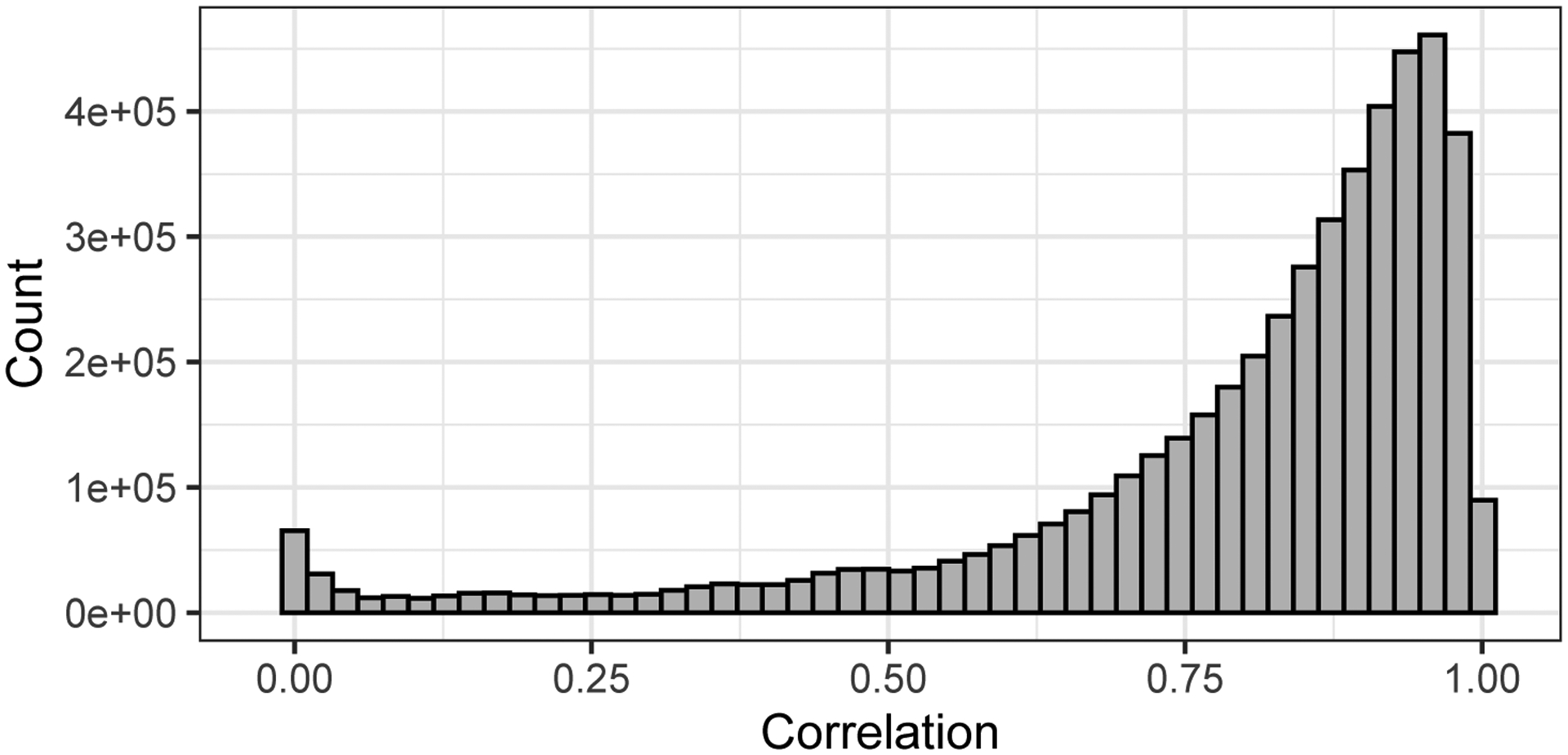
Pairwise correlation between each of the 777 molecular descriptors in ToxCast for the chemicals profiled.

Dose response data and molecular structure are the two sources of information in ToxCast relevant to addressing our goal. Explicitly, chemical i in ToxCast has two relevant pieces of information: the vector of response observations at D doses y_i = [y_i(d₁),…, y_i(d_D)]′, and the vector of S molecular features x_i = [x_i1, …, x_iS]′. Observations y_i are sparse, noisy and not on a regular grid. For an example, see Figure 2; Chlorobenzilate has 54 observations at 11 unique doses, yet 5-Methyl-1H-benzotriazole only has three doses with one observation each. Not all aspects of the feature space (i.e., not all entries in x_i) are likely to be relevant to the toxicological response.

Fig. 2.

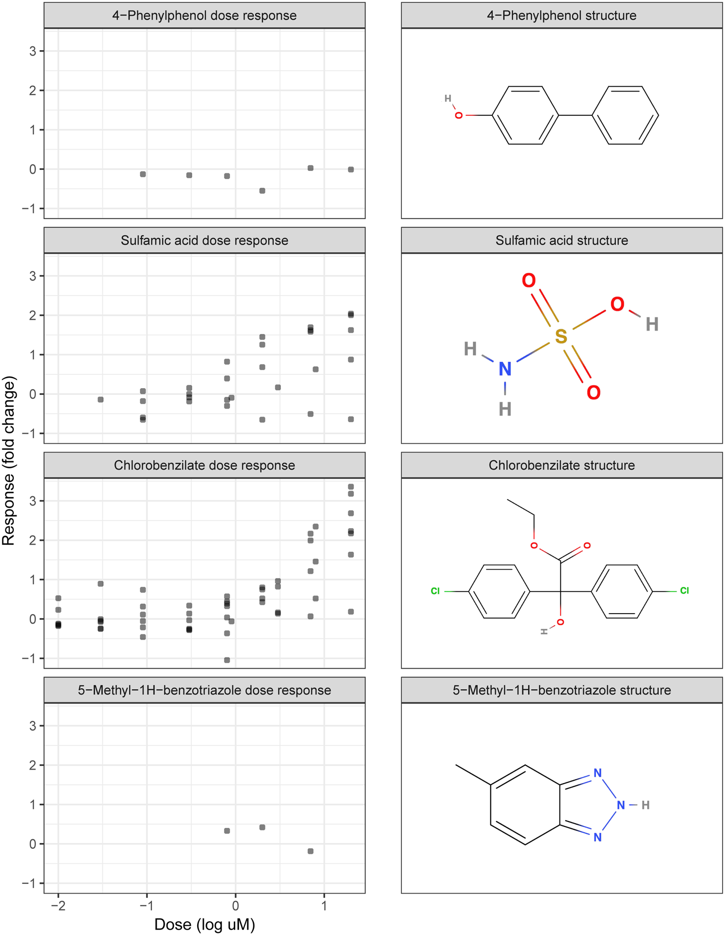
Left: Dose response data for example chemicals from the ToxCast ATG PXR assay (i.e., y_i). Right: 2D chemical structure diagrams for example chemicals (converted from SMILES into x_i using the Mold2 software).

Response variables in ToxCast are assay specific. Assays in ToxCast each measure a single endpoint, for example, the binding to a certain receptor protein, or the transcription of a target gene. The specific assay endpoint considered in our real-data example, the AttaGene pregnane X receptor (PXR) assay, records the fold-change values in the activity of the nuclear pregnane X receptor for drug-treated vs. control-treated human hepatic cells (specifically, a HG19 subclone of HepG2). Dimethyl sulfoxide (DMSO) is used as the negative control. The response is measured via reporter RNAs that are produced proportionately to the activity of corresponding transcription factor (here, PXR). This assay has been shown to be related to the body’s response to toxic substances (Kliewer, Goodwin and Willson (2002)), so a higher response value for this assay endpoint can be interpreted as higher level of toxicity.

This work makes no monotonicity assumptions on the shape of the response. There is a nonzero baseline activity level of the nuclear pregnane X receptor in unstimulated hepatic cells, so both induction and suppression of the activity of this transcription factor are possible outcomes in response to stimulation, rendering a positive monotonicity constraint unsuitable. Furthermore, the lack of any monotonicity constraint (not specifically a positive one) leaves open the possibility for a biphasic response such as hormesis to be fit.

The tool used to quantitatively summarize a chemical’s molecular structure is Mold2 (Hong et al. (2008)), which generates a set of 777 numeric descriptors using the simplified molecular-input line-entry system (SMILES) specification (Weininger (1988)); see Figure 3 for select Mold2 output for an example chemical, and Hong et al. (2012) for a discussion of the use of Mold2 in quantitative structure–activity relationship (QSAR) models.

Fig. 3.

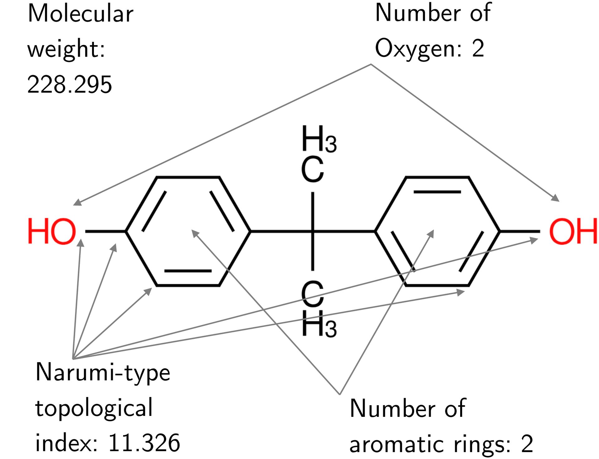
Numeric values for select Mold2 traits of Bisphenol A (BPA). The chemical formula for BPA is C₁₅H₁₆O₂, and its SMILES descriptor is CC(C)(C1=CC=C(C=C1)O)C2=CC=C(C=C2)O.

In order to coherently model both structural and toxicological response variation, we propose a Bayesian partially Supervised Sparse and Smooth Factor Analysis (BS³FA) model. The model assumes structured variation in the molecular features x_i is driven by two sets of latent factors: call these F_x-specific and F_shared. F_x-specific is unrelated to the toxicological response and is responsible for structured molecular variability that does not impact toxicity. F_shared is assumed to drive variation in the toxicological response y_i and thus is responsible for structured molecular variability that does impact toxicity. The directions spanned by these two sets of latent factors can be thought of as the “toxicity-irrelevant” and “toxicity-relevant” spaces, respectively.

Chemical similarity can be characterized by proximity in this latent toxicity-relevant space, enabling a measure of distance with uncertainty quantification that is adapted to the particular response space of interest. Such a metric is powerful because: (1) it is based on a subspace driving variation in activity, whereas proximity with respect to the full set of molecular descriptors does not necessarily mean proximity with respect to activity (Martin, Kofron and Traphagen (2002), Nikolova and Jaworska (2003)) and (2) it is purely statistically derived, requiring no knowledge of the fundamental chemical and biological processes responsible for the activity, as such information is not always available. Such an activity-relevant distance metric could be used by toxicologists in the design of diverse chemical libraries or to select new compounds to augment a screening collection such as ToxCast.

As with function-on-scalars regression approaches, the BS³FA model allows for the prediction of activity profiles for chemicals that have not yet been screened in ToxCast. It does so by embedding the full set of molecular features for a new chemical into the latent toxicity-relevant feature space F_shared and then projecting this embedding out to the activity space. The predicted dose-response profiles can be used to generate point and interval estimates for common univariate toxicological outcomes of interest, such as 50% activity concentration (AC50), maximum activity or the area under curve (AUC), which can be used in place of the as of yet unobserved in vitro results for that chemical.

The rest of the paper is organized as follows. First, we describe existing and potential approaches to modeling chemical structure and activity. Then, the BS³FA model is described, and its performance is compared to that of existing algorithms on simulated data sets. Next, a detailed analysis of the motivating application data set is considered, where the BS³FA model is run with Mold2 chemical features and the Attagene PXR assay from the ToxCast data set as input data. Finally, the results are discussed and future areas of research are highlighted.

2. Background.

QSAR models (see Figure 4) are based on the assumption that chemicals with similar features are likely to have similar effects. The ToxCast data poses two main challenges for QSAR modeling. First, it is often not trivial to characterize similarity in activity-relevant chemical feature space well (Martin, Kofron and Traphagen (2002), Nikolova and Jaworska (2003)). Second, the majority of QSAR models aim to relate structure to a summary of the data across times/doses (e.g., Liu et al. (2011), Patel et al. (2014), O’Connell and Lock (2019)) rather than to the full dose response curves.

Fig. 4.

Quantitative Structure-Activity Relationship (QSAR) models predict toxicity as a function of chemical structure.

We discuss these considerations in the context of existing QSAR models and other related approaches not yet applied to QSAR models. To the authors’ knowledge, no existing approaches are able to address the challenge of learning a low-dimensional representation for multivariate feature data x_i partially supervised by sparse functional data y_i.

2.1. QSAR approaches for dose response profiles.

Two existing QSAR approaches have attempted to relate molecular descriptors to full dose response curves (Low-Kam et al. (2015), Wheeler (2019)). In Low-Kam et al. (2015), a Bayesian regression tree is defined over functions where each leaf represents a different dose-response surface. This method was used to learn about the relationship between chemical properties and observed dose-response. However, the model lacks the ability to scale to the numbers of chemicals and molecular descriptors considered here. Furthermore, predictive performance was found to be lacking in leave-one-out analysis. Finally, the code was designed under the assumption that each chemical would be tested at the same doses with the same number of replicates at each dose.

The Bayesian additive adaptive basis tensor product (BAABTP) model (Wheeler (2019)) is designed purely for prediction. It learns basis functions via independent Gaussian process (GP) priors over the molecular structure space and the dose space. In the model, step one is to perform PCA on the set of Mold2 chemical descriptors. Step two is to use the principal feature space explaining 95% of the variation in this Mold2 descriptor set as the input to the distance kernel for the molecular structure GPs.

The BAABTP model has two major problems, both stemming from the Gaussian process prior over chemical structure. First, the model becomes computationally intractable when the number of chemicals increases past a few thousand—the number of chemicals tested in the ATG PXR assay has increased from under 1000 up to nearly 4000 in the time since the data were analyzed in Wheeler (2019), and this number will only continue to grow. Second, the GP priors over chemical structure rely on a concept of molecular distance based on total, rather than toxicity-relevant, variability. Mold2 descriptors are a numeric representation of the 2D structure of a chemical. Thus, while the leading principal components (PCs) account for the majority of structural variability across chemicals, these leading PCs may not be those most relevant to toxicity. Figure 5 illustrates this phenomenon, showing that chemicals may be close in PCA-based structure space but distant in response space. In other words, similarity in directions of highest structural variability does not necessarily correspond to similarity in directions of highest activity variability.

Fig. 5.

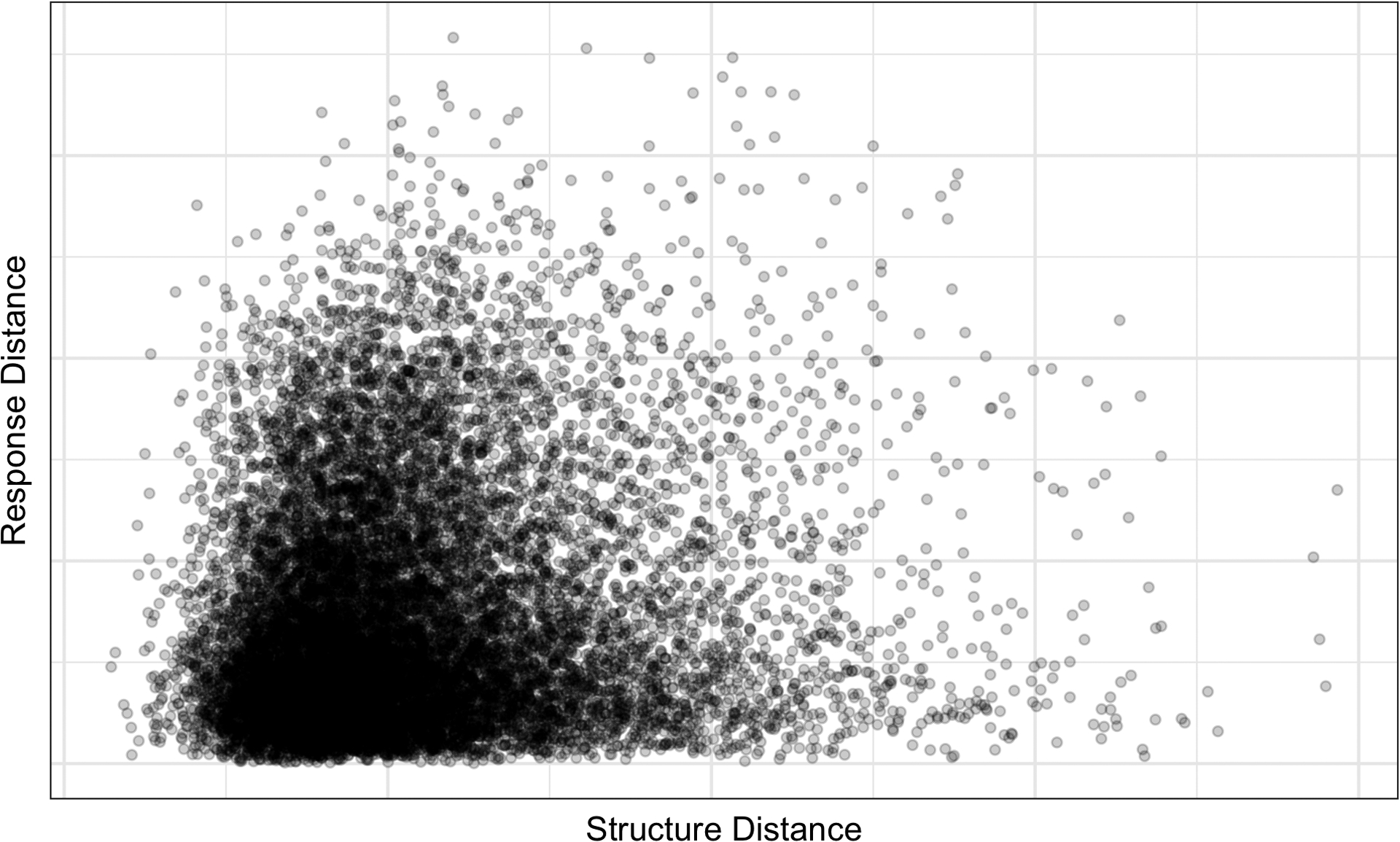
Relationship between chemical “structure distance” and chemical “activity distance” when PCA and functional PCA (FPCA) are performed independently on the Mold2 chemical structures and the ToxCast dose-response curves. Each point on the graph shows the Euclidean distance between the (functional) principal component scores accounting for 95% of the variability in the data for one pair of chemicals on the (y-) x-axis.

2.2. Toward the proposed approach.

Supervised and sparse functional PCA (supSFPCA) (Li, Shen and Huang (2016)) defines a hierarchical model to provide supervision for dimension reduction of functional data by another multi-output data source. A small modification to the penalty term used in this algorithm would allow for the opposite relation (i.e., to supervise the dimension reduction of the feature data x_i by functional dose-response data y_i), but the larger issue is that the supSFPCA algorithm is designed such that the algorithm finds directions that maximize unexplained variability in x_i (i.e., what isn’t accounted for by y_i) rather than finding directions that maximize variability explained by y_i. As such, this algorithm is of little use for prediction or for learning about directions of variability of most relevance for toxicity.

The Bayesian latent factor regression model (LFRM) of Montagna et al. (2012) characterizes y_i as a linear combination of a high-dimensional set of basis functions. The basis functions themselves are fixed rather than learned which means that a large number of basis functions must be included in order to flexibly model many possible functional shapes. This high number of bases drives the choice to use a latent factor regression model on the basis coefficients rather than defining a regression model on the basis coefficients themselves. Thus, the latent factor scores enter the model in a “lower” layer in Montagna et al. (2012) than they do in BS³FA and are a linear function of covariates x_i rather than being assumed to drive variability in x_i. A shrinkage prior is placed on the regression terms associated with the latent factor scores in the model, allowing covariates to impact certain facets of the functional response while others are shrunk to zero.

Our approach was inspired by the conceptual goal of separating variability shared by x_i and y_i into toxicity-relevant, toxicity-irrelevant and noise components, similar to the idea behind the joint and individual variation explained (JIVE) method (Lock et al. (2013)), and an analogous joint Bayesian factor model (JBFM) (Ray et al. (2014)). We utilize similar shrinkage tools as LFRM and the Bayesian function-on-scalars regression (B-FOSR) of (Kowal and Bourgeois (2020)), implementing sparsity-inducing coefficient-level priors to account for the high-dimensional predictors and imposing ordered sparsity so as to reduce the impact of the choice of latent subspace dimension. Unlike LFRM and like B-FOSR, the BS³FA model learns a flexible basis for the functional response rather than prescribing a set of basis functions. Like LFRM, JBFM, and B-FOSR, modeling takes place within a Bayesian framework for unified parameter estimation, prediction and uncertainty quantification about posterior summaries of interest, and model components are identifiable.

Like many of the approaches described in the previous sections, our model is able to predict the dose-response profiles for new chemicals. Unlike previous models, our model is able to learn a toxicity-relevant subspace underlying variation in both the chemical structure and toxicological response. This subspace can be used to describe a statistically-driven activity-relevant distance between chemicals. It can also provide insight into how toxicity-relevant variability manifests across both molecular structure and dose-response profiles.

3. BS³FA model.

Figure 6 gives a visual representation of the BS³FA model. BS³FA is able to: (1) learn a linear low-dimensional latent space underlying both molecular structure and activity, (2) develop a distance metric for chemicals relying only on molecular structures relevant to toxicity, (3) handle responses observed at a sparse, irregularly spaced set of doses and (4) enable activity predictions for chemicals having no observed dose-response information.

Fig. 6.

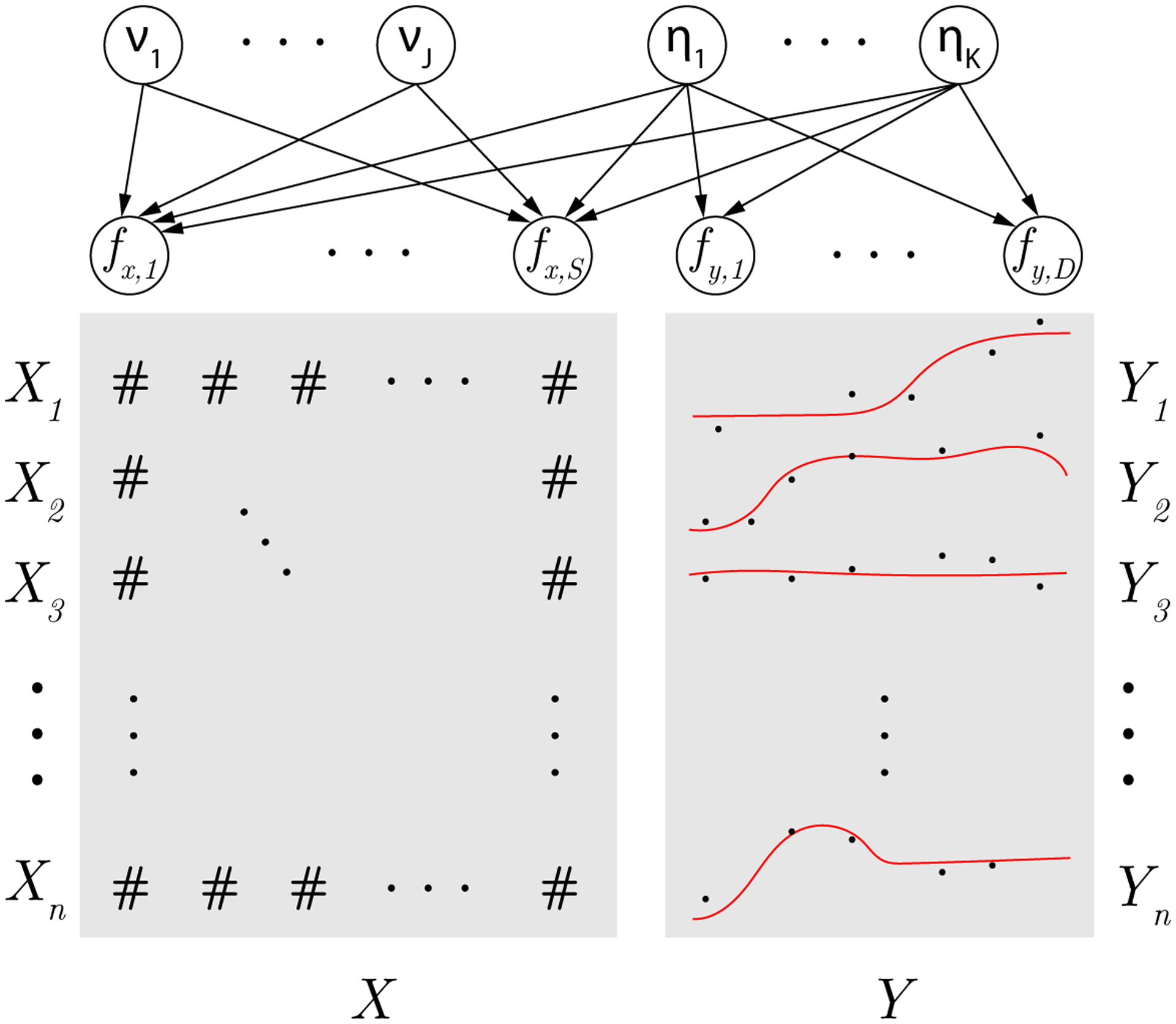
Visual representation of the BS³FA model. Entries in X are the chemical feature descriptors from Mold2, while entries in Y are noisy realizations of an underlying smooth dose-response curve. Observations f_x,1, …, f_x,S are the true mean of the chemical features and f_y,1, …, f_y,D are the true mean of the dose-response values. Latent variables η₁, …, η_K, the underlying toxicity-relevant factors, are shared, and ν₁, …, ν_K, the underlying toxicity-irrelevant factors, are specific to the chemical features. Arrows denote probabilistic dependency.

3.1. Model specification.

The characteristics of chemical structure and toxicological response can likely be summarized using fewer descriptors.

As shown in Figure 1, many molecular descriptors tend to exhibit high correlation. Furthermore, their realized value can often be attributed to some underlying trait of the molecule (e.g., many descriptors are largely driven by molecule size; the descriptors number of carbon, number of oxygen, molecular weight and number of atoms in the molecule all have pairwise correlation above 0.9). Similarly, dose-response profiles exhibit a somewhat limited range of shapes, suggesting possibly a few underlying functional “building blocks” comprising variation in activity.

Factor modeling is a means by which to model variability in high-dimensional data via an underlying lower dimensional subspace. For some set of observations ${\left\{z_i\right\}}_{i=1}^N$, where z_i is the P-dimensional vector of measurements for observation i, the traditional (nonjoint) factor model is

$$\begin{array}{l}{\mathit{\text{z}}}_i=\Lambda {\mathit{\text{η}}}_i+{\mathit{\text{ϵ}}}_i,{\mathit{\text{η}}}_i~{\text{N}}_K(0,I),{\mathit{\text{ϵ}}}_i~{\text{N}}_P\left(0,{\Sigma }_0\right),\\ {\Sigma }_0=\text{diag}\left({\sigma }_1^2,\dots ,{\sigma }_P^2\right),i=1,\dots ,N.\end{array}$$ (1)

The prior induced on the latent z_i by integrating out the unknown η_i is then

$${\mathit{\text{z}}}_i~\text{N}\left(0,\Lambda \Lambda \text{'}+{\Sigma }_0\right),$$ (2)

yielding a lower dimensional representation of the covariance between measurements.

Chemical features are often nonnormal (e.g., count, skewed continuous or binary).

Many chemical descriptors from Mold2 are counts of particular elements (number of carbon, number of oxygen, etc.).

In order to allow this framework to encompass data of mixed type, define

$$x_{is}=f_s\left(z_{is}\right),i=1,\dots ,N,s=1,\dots ,S.$$ (3)

The particular link function f_s depends on the feature specification, allowing for mixed scale data via selection of an appropriate link by scale and type. Let f_s(z_is) = z_is or f_s(z_is) = log(z_is) for continuous x_is, with the latter chosen for strictly positive and positively skewed cases. Let f_s(z_is) = 1(z_is > 0) for binary x_is, where 1(·) is an indicator function taking the value of 1 when the argument is true and 0 when the argument is false. Categorical variables may be incorporated under this framework by transforming the C categories into C − 1 binary variables indicating whether or not the categorical value for that individual took a given nonbaseline category value; the result is that either none or one of the C − 1 variables will take on a value of 1. Finally, for count x_is, which may or may not be zero-inflated, let f_s(z_is) be a rounding operator such that f_s(z_is) = 0 if z_is < 0 and f_s(z_is) = t if t – 1 ≤ z_is < t, as specified in Canale and Dunson (2013).

There is likely a shared low-dimensional space underlying chemical features and activity.

BS³FA assumes that some underlying factors explain all of the variation in the dose-response curves and, jointly, part of the variation in the associated chemical features. Recall z_i and y_i denote S- and D-dimensional (latent) continuous features and observed dose-response curves, respectively, for observation i. Assume that the indexing of y_i is such that the function is “in order” (for the ToxCast data, in order means that the D unique doses are sorted such that the doses increase with index). Also, for notational convenience assume that functional data y_i are only observed once per index (the case of notationally awkward multiply observed doses is explicitly addressed in the Gibbs sampler described in the Appendix). BS³FA models

$$\begin{array}{l}\underset{S\times 1}{{\mathit{\text{z}}}_i}=\underset{S\times 1}{{\mathit{\text{μ}}}^z}+\underset{S\times K}{\Theta }\underset{K\times 1}{{\mathit{\text{η}}}_i}+\underset{S\times J}{\Xi }\underset{J\times 1}{{\mathit{\text{v}}}_i}+\underset{S\times 1}{{\mathit{\text{e}}}_i},\\ \underset{D\times 1}{{\mathit{\text{y}}}_i}=\underset{D\times 1}{{\mathit{\text{μ}}}^y}+\underset{D\times K}{\Lambda }\underset{K\times 1}{{\mathit{\text{η}}}_i}+\underset{D\times 1}{{\mathit{\text{ϵ}}}_i},\\ i=1,\dots ,N.\end{array}$$ (4)

The form of the above model is that of a set of linked factor models. Note that, although there are three non-error component pieces aside from the global mean terms (namely, Θη_i, Ξν_i, and Λη_i), there are only two unique factor vectors: η_i and ν_i. These factors are highly interpretable. The term η_i represents the shared latent space underlying structured variability in both z_i and y_i (note that it appears in both factor models). In the expression for y_i, it is the sole factor vector and in that for z_i it is one of two factor vectors. Thus, it is responsible for all structured variation in y_i but only part of the structured variation in z_i. The term ν_i represents structured variation in z_i that is unrelated to y_i.

By not including unique response-only factors (i.e., factors not assumed to underlay chemical structure) in the mean formulation for y_i, the model assumes that the mean dose-response curves can be constructed from factors that are all also present in the chemical feature data. Making this assumption allows for easier identification and accurate estimation of parameters associated with chemical features predictive of activity, which is the main goal of this work. The trade-off of this assumption is that if the feature set is inappropriate (e.g., not containing enough information by which to estimate activity) and/or the dose-response profiles are truly driven by some individual factors not related to chemical features, then the estimates for new chemicals may be overconfident and the model fit may be poor. The shrinkage prior on Θ, discussed in a later section, offers some mitigation of this risk.

If z_i and y_i are mean-centered prior to analysis, fix μ^z and μ^y to be zero vectors for computational savings. In practice, mean centering is not sensible to perform for count or binary features (i.e., for s s.t. x_is is binary or count). For noncentered x_is, ${\mu }_s^z$ is given a Cauchy prior expressed as ${\mu }_s^z~\text{N}\left(0,{\zeta }_s^{-1}\right)$, ζ_s ~ Ga(0.5, 0.5). Since the Cauchy distribution has high density around zero and heavy tails, it is able to capture meaningful signals while still encouraging shrinkage. If the y_i are not mean-centered, μ^y is given a GP prior analogous to the prior placed on the columns of Λ, discussed in the next section.

In the above model the mean of z_i is μ^z + Θη_i + Ξν_i, and e_i is a term for unstructured noise in z_i. Similarly, the mean of y_i is μ^y + Λη_i, and ϵ_i is the unstructured noise term for y_i. The priors on the shared factors {η_i}, the X-specific factors {ν_i} and error terms are set to be those typically used in factor analysis,

$$\begin{array}{l}{\mathit{\text{η}}}_i~{\text{N}}_K(0,I),{\mathit{\text{v}}}_i~{\text{N}}_J(0,I),\\ {\mathit{\text{e}}}_i~{\text{N}}_S\left(0,{\Sigma }_X\right),{\Sigma }_X=\text{diag}\left({\sigma }_{X,1}^2,\dots ,{\sigma }_{X,S}^2\right),\\ {\mathit{\text{ϵ}}}_i~{\text{N}}_D\left(0,{\Sigma }_Y\right),{\Sigma }_Y=\text{diag}\left({\sigma }_Y^2,\dots ,{\sigma }_Y^2\right).\end{array}$$ (5)

Homoscedastic variance is assumed for dose-response curves Y. Fix ${\sigma }_{X,s}^2$ to 1, if feature s is binary, for reasons of identifiability.

Note that, as of yet, we have not fully addressed how to structure the factor model in light of the functional nature of the y_i, nor the issue of many entries in z_i likely being unrelated to y_i. The following sections will describe how structure can be imposed on Λ and Θ, respectively, in light of these considerations.

The dose-response curve data are functional in nature.

Figure 2 shows the noisy observations from a set of example chemicals, but the underlying signal represents a smooth curve relating chemical dose to response.

For functional data it is preferable to have each loading vector (i.e., each column of Λ) itself be functional. The desired smoothness of the mean curves underlying noisy observations y_i can thus be imposed via the choice of smooth priors on the loading matrix Λ. Let λ_k denote the kth column of Λ, so

$$\Lambda =\left[\begin{array}{cccc}\mid & \mid & & \mid \\ {\mathit{\text{λ}}}_1& {\mathit{\text{λ}}}_2& \dots & {\mathit{\text{λ}}}_K\\ \mid & \mid & & \mid \end{array}\right].$$

In order to learn rather than prescribe smooth bases, columns of Λ are modeled as D-dimensional Gaussian processes,

$${\mathit{\text{λ}}}_k~\mathcal{G}\mathcal{P}\left(0,c_k(\cdot )\right),c_k\left(d,d^{\prime }\right)={\alpha }_k^2{e}^{-\frac{{\left(d-d^{\prime }\right)}^2}{2{\ell }^2}},k=1,\dots K.$$ (6)

The Gaussian process function variance ${\alpha }_k^2$ is comprised of two components: a global inverse variance term ϕ and a column-specific inverse variance term τ_k. The column-specific inverse variance term τ_k utilizes the multiplicative gamma process prior of Bhattacharya and Dunson (2011), leading to stochastic shrinkage of columns of Λ toward 0 by index:

$$\begin{array}{l}{\alpha }_k^2={\left(\varphi {\tau }_k\right)}^{-1},{\tau }_k=\prod _{h=1}^k{\delta }_h,k=1,\dots K,\\ \varphi ~\text{Ga}\left(g_{\varphi }/2,g_{\varphi }/2\right),{\delta }_1~\text{Ga}\left(a_1,1\right),{\delta }_h~\text{Ga}\left(a_2,1\right),h\ge 2.\end{array}$$ (7)

Following the note by Durante (2017) on hyperparameter selection, set a₁ = 2.1 and a₂ = 3.1 in equation (7). The value of g_ϕ, the hyperparameter for the global function precision of the GP, should be chosen to reflect the scale of the data.

This stochastic shrinkage leads to an effective truncation of the factors and an automatically learned dimension of the latent space, so long as K is chosen large enough (whether K is adequately large can be assessed by monitoring the convergence of ${\alpha }_k^2$ to 0 as k approaches K). To see why, consider the model for y_i written in expanded form: y_i = λ₁η_i,1 + λ₂η_i,2 + ⋯ + λ_Kη_i,K + ϵ_i. Assuming K is large enough, as k approaches K, the vector λ_k should be approximately the 0-vector, meaning that many of the later terms will contribute negligibly to the mean of y_i; see Figure 7 for a visualization of Λ and column shrinkage.

Fig. 7.

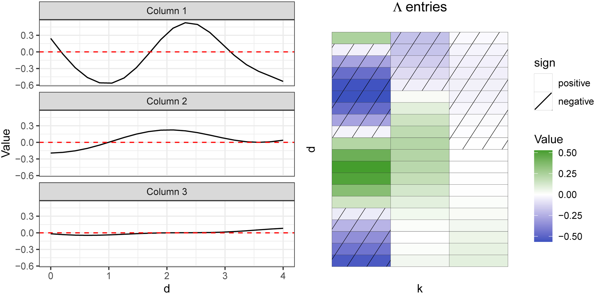
Visualization of the smoothness and the shrinkage of columns of an example D = 20 by K = 3 loadings matrix Λ. The effect is an automatic truncation of the number of factors in the model and a learned latent dimension. In this figure, columns of Λ were sampled using the kernel in equation (6) with ℓ² = 1 and ${\alpha }_k^2$ being 1, $\frac{1}{25}$, $\frac{1}{400}$ for k = 1, 2, 3, and the indices d corresponding to the length-20 vector from 0 to 4, inclusive. Note that as ${\alpha }_k^2$ decreases, the functions tend to flatten.

The linked nature of the factor models leads to an induced prior on the covariance between elements of z_i and elements of y_i; specifically, Cov(z_is, y_i(d)) = Σ_k θ_skλ_k(d). The GP prior on columns of Λ implies that the covariance between a given feature and a given point on the dose-response profile is a smooth function of dose, a desirable model characteristic.

Many features are likely unimportant for certain aspects of chemical activity.

That is, if a set of chemical descriptors has not been carefully selected to be toxicity-relevant, it is unlikely that all are related to the shape of the dose-response curves. Even if all features are toxicity-relevant, it is plausible that features will impact different pieces of the toxicity profile (e.g., some features may impact the steepness of the dose-response, while others may impact the height of the final plateau). The way to encourage such a relationship is via elementwise shrinkage (i.e., zeros in entries) of the factor loadings matrix Θ.

Shrinkage on elements θ_sk of Θ is desirable because it is likely that for a given factor many features have negligible impacts on the associated component of the functional y_i. Explicitly,

$$\Theta =\left[\begin{array}{ccccc}{\theta }_{11}& {\theta }_{12}& {\theta }_{13}& \dots & {\theta }_{1K}\\ {\theta }_{21}& {\theta }_{22}& {\theta }_{23}& \dots & {\theta }_{2K}\\ ⋮& ⋮& ⋮& \ddots & ⋮\\ {\theta }_{S1}& {\theta }_{S2}& {\theta }_{S3}& \dots & {\theta }_{SK}\end{array}\right].$$

There is a very rich literature proposing elaborate shrinkage and sparsity priors for factor loadings (e.g., Knowles and Ghahramani (2011), Meng et al. (2010), Pati et al. (2014), Yoshida and West (2010)). We opt for a horseshoe prior (Carvalho, Polson and Scott (2010)) modified for simple sampling (Makalic and Schmidt (2016)) on entries θ_sk of Θ,

$$\begin{array}{l}{\theta }_{sk}~\text{N}\left(0,{\beta }^2{\gamma }_{sk}^2{\tau }_k^{-1}\right),\\ {\beta }^2\mid t~\text{IG}(1/2,1/t)\\ {\gamma }_{sk}^2\mid b_{sk}~\text{IG}\left(1/2,1/b_{sk}\right)\\ \left\{b_{sk}\right\},t~\text{IG}(1/2,1),\\ s=1,\dots S,k=1,\dots K.\end{array}$$ (8)

The horseshoe component of this prior is in the hierarchical hyperprior on global variance term β² and local variance term ${\gamma }_{sk}^2$. The column-specific variance ${\tau }_k^{-1}$ applies stochastically increasing shrinkage as column index increases; see Figure 8 for a visualization of Θ and column shrinkage.

Fig. 8.

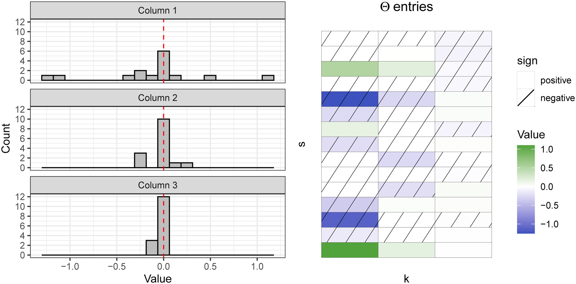
Visualization of elementwise sparsity and the shrinkage of columns of an example S = 15 by K = 3 loadings matrix Θ. The effect is an automatic truncation of the number of factors in the model and a learned latent dimension. In this figure, columns of Θ had column-specific variance ${\tau }_k^{-1}$ being 1, $\frac{1}{25}$, $\frac{1}{400}$ for k = 1, 2, 3.

Recall Cov(z_is, y_i(d)) = Σ_k θ_skλ_k(d). The shrinkage prior on entries of Θ allows for the possibility that a given chemical feature may not have a contribution from some or any of the latent factors (i.e., that θ_sk for such feature/factor combinations is near 0). In this case the covariance between the feature and points along the dose-response profile will not depend on those factor(s). In the extreme case that the sth feature is unrelated to toxicity, θ_sk should be shrunk toward zero for all k, leading z_is and y_i(d) to be uncorrelated.

The dimension of the latent space underlying the dose-response curves and of that underlying toxicity-relevant features should be the same.

The same column-specific precision ${\tau }_k^{-1}$ is used for both Θ and Λ, so relative column shrinkage is applied consistently across the two matrices. The result is the same effective truncation on the number of latent factors in the joint space. This specification, along with the common η_i, is what allows the shared directions of variability between y_i and x_i to be learned. Distance can be defined over the η-vector with elements η_k weighted by precision ${\tau }_k^{-1}$ to give a sense of closeness in “η space” that reflects the true amount of information contained in each latent direction.

There is additional variability in chemical structure beyond that which impacts chemical activity.

Unless all chemical features were carefully hand-selected to be toxicity relevant for the specific assay considered in the model (a tall task and unlikely to be completely true no matter how careful the selection), accounting for variability in z_i shared with y_i will not capture all structured variability in chemical features.

After accounting for the variability in z_i shared with y_i (via latent factor η_i), z_i may still have structured variation due to individual latent factor ν_i. Let ${\mathit{\text{z}}}_i^{*}={\mathit{\text{z}}}_i-\Theta {\mathit{\text{η}}}_i$. Then, ${\mathit{\text{z}}}_i^{*}=\Xi {\mathit{\text{v}}}_i+{\mathit{\text{e}}}_i$ which once again looks like a traditional factor model. The direct application of priors in Bhattacharya and Dunson (2011) is used for elements of Ξ. Specifically, elements ξ_s,j of Ξ are given prior

$$\begin{array}{l}{\xi }_{s,j}\mid {\kappa }_{sj},{\omega }_j~\text{N}\left(0,{\kappa }_{sj}^{-1}{\omega }_j^{-1}\right),{\omega }_j=\prod _{h=1}^j{\zeta }_h,s=1,\dots S,j=1,\dots J,\\ {\kappa }_{sj}~\text{Ga}\left(g_{\kappa }/2,g_{\kappa }/2\right),{\zeta }_1~\text{Ga}\left(m_1,1\right),{\zeta }_h~\text{Ga}\left(m_2,1\right),h\ge 2.\end{array}$$ (9)

Stochastic column-specific shrinkage via the ${\omega }_j^{-1}$ term removes the need to select an ideal number of factors J and allows for simply selecting J “large enough.” This formulation also allows for efficient Gibbs sampling of the posterior. Following the note by Durante (2017) on hyperparameter selection, set m₁ = 2.1 and m₂ = 3.1 in equation (9). The value of g_κ, the hyperparameter for the entry-level precision terms of Ξ, should be chosen to reflect the scale of the data.

If there is in fact, no additional variability in z_i beyond that shared with y_i, the following specification allows for all columns of Ξ to be shrunk to 0-vectors. This case reduces to a fully joint factor model in which all variability in z_i is shared with y_i.

Chemical activity is not necessarily measured on a fully observed, regularly spaced grid.

There are a handful of common dose measurements at which the majority of chemicals are measured (see Figure 11), but there are many chemicals whose observations are less regular. Furthermore, some chemicals have multiple observed dose-response curves.

Fig. 11.

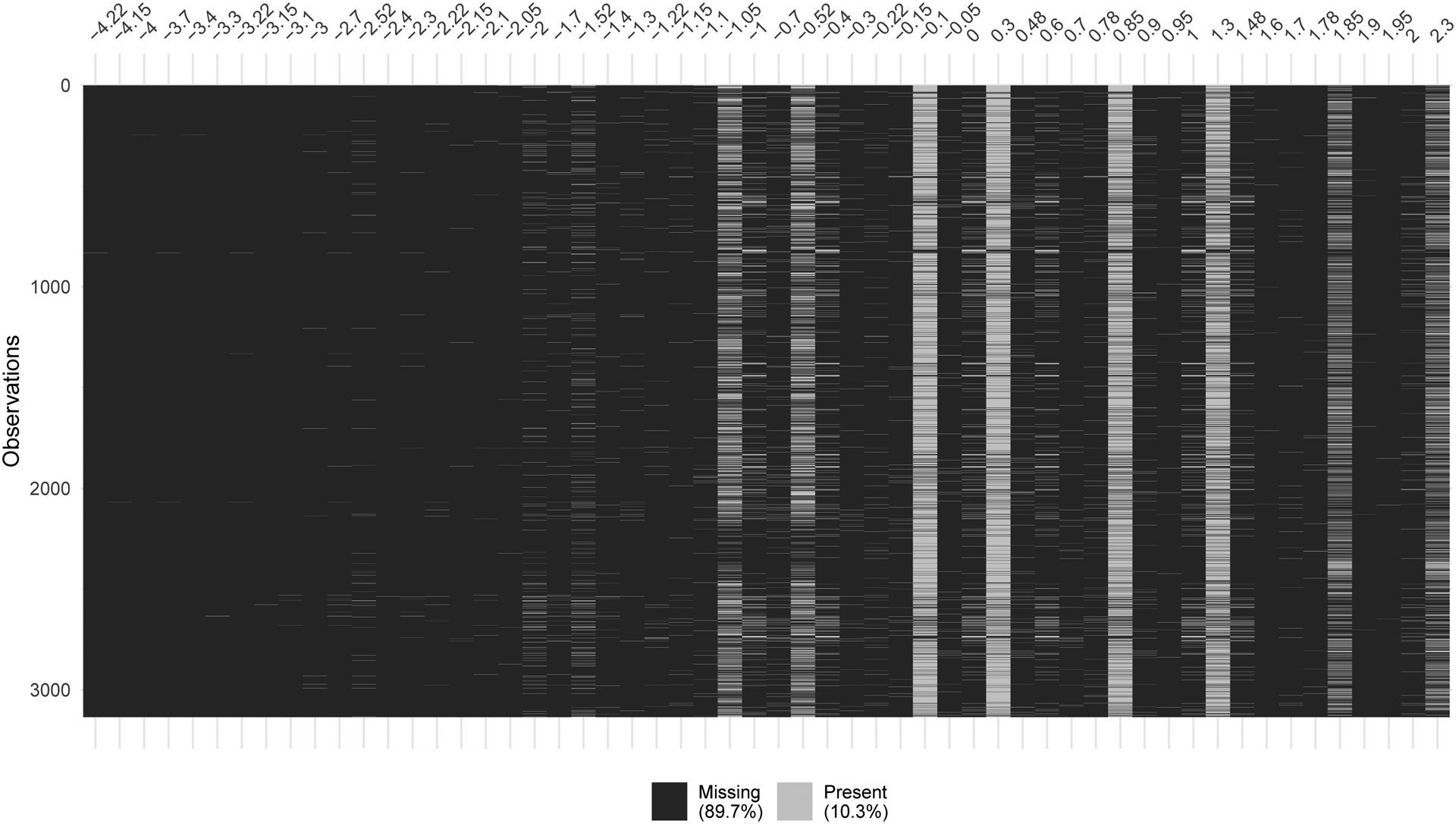
Missingness by dose for each chemical in the analysis. Each row is corresponds to a chemical and each column to a dose value (sorted in ascending order). Note that very few chemicals have observations below −2 log uM.

The issue of irregular spacing between the unique values associated with the indices is handled automatically via the use of GPs for modeling columns of Λ. The covariance between points is defined by the kernel for any pair of input values (see equation (6)) and not dependent on a regular measurement grid.

Toxicologists may wish to report different components and/or summaries of predicted dose-response curves.

For example, they may be interested in the dose value at which the response first exceeds some threshold, the maximum response value reached, the area under the curve, etc. Each of these summaries provides different information about the dose-response relationship. An advantage of a Bayesian formulation is that we can obtain posterior samples for any functional of the dose-response curve trivially, with these samples then used to obtain point and interval estimates.

3.2. Posterior computation.

The posterior for the BS³FA model is not available in closed form. However, closed form full conditional distributions of the parameters associated with the model allow the use of a straightforward Gibbs sampler for these draws. Samples obtained directly from this Markov chain Monte Carlo (MCMC) algorithm allow for the calculation of posterior means, simultaneous bands (Meyer et al. (2015)), and credible intervals for identifiable model components, including the predicted mean, covariance, and noise variance of X and Y. A post-processing step to resolve rotational ambiguity and account for label/sign switching allows for identifiability of the individual model components, including the factor scores η and loadings Λ and Θ (code modified from https://github.com/poworoznek/sparse_bayesian_infinite_factor_models). Full details on the Gibbs sampler steps and initialization are included in the Supplementary Material (Moran et al. (2021)).

3.3. Code base and reproducibility.

Code for simulating data and sampling from the BS³FA model, along with a user manual, are made available at https://github.com/kelrenmor/bs3fa. A hands-on demonstration of the package is available at https://www.youtube.com/watch?v=qLyxBQ-sVcY. Code specific to this paper (i.e., to reproduce the simulations, figures, and results) is provided in the Supplementary Material (Moran et al. (2021)).

3.4. Simulation study.

Simulation studies were performed in order to assess the ability of BS³FA to learn the true toxicity-relevant distance between chemicals, its predictive performance and the model fit. Two broad categories of simulations were performed: first, those in which the true data generating process aligns with model assumptions (i.e., when data are simulated from a partially shared latent factor model) and when it does not (i.e., when data are simulated from something other than a factor model). In the former category we also assess how well model subcomponents can be learned.

For all simulations, 25% of simulated “chemicals” are held out. That is, rather than with-holding 25% of dose-response observations across chemicals, we withhold all dose-response data for each hold-out chemical. For distance performance, BS³FA is compared to Euclidean distance using all features, using the features selected in the B-FOSR model from the fosr R package via an extension of the decision analytic approach of Hahn and Carvalho (2015) to the functional data setting (Kowal and Bourgeois (2020)), using the principal component scores explaining 95% of the variability in the data found in PCA, and using the selected variables from a frequentist FOSR using the fosr.vs() function (FOSR-VS) from the refund R package with the PC scores used as inputs. PC scores were used instead of the full set of features for FOSR-VS because the fosr.vs() function returned an error saying the dimension of y_i was not high enough relative to x_i (i.e., that D was too small relative to S) when the full feature set was used. The performance of each method is compared by computing the correlation between predicted and true distance, a choice made because the scale of distance varies across methods and, by virtue of the structure of the simulated data, we don’t expect any extreme outliers in this space. For predictive performance, BS³FA is compared to the BAABTP model (Wheeler (2019)), B-FOSR, FOSR-VS, and least absolute shrinkage and selection operator (LASSO) using each covariate, dose and all pairwise interactions.

For simulations in which the true data generating process aligns with model assumptions, the true dimension of the latent toxicity-relevant space K was varied, taking values 1, 3 and 5. For each K, the true dimension of the latent toxicity-irrelevant space J was varied from 0 to 20 in intervals of five. At each combination of K and J, 100 data sets were simulated with N = 300, D = 10, and S = 40. For roughly half of the chemicals in each data set, η_i was set to a zero vector for that chemical (i.e., for each simulated data set there was a 50% chance that any given chemical was inactive). Further simulation details are provided in the Supplementary Material (Moran et al. (2021)). Overall, the model does quite well at capturing the structure of the noise variance and the true components Λ and Θ.

Figure 9 shows the correlation between entries in the true pairwise distance matrix (i.e., the Euclidean distance between true latent factors η) and the predicted pairwise distance matrix for holdout chemicals. We see that even in the case of small J, performing PCA on the S-dimensional X matrix obscures the true distance in the latent space. As J increases, the correlation between the chemical distance in the true η and that in either PCA space or Euclidean space drops quickly. This phenomenon also occurs for distances computed via variable selection using B-FOSR or FOSR-VS. The BS³FA model has stable high correlation across all values of J and K.

Fig. 9.

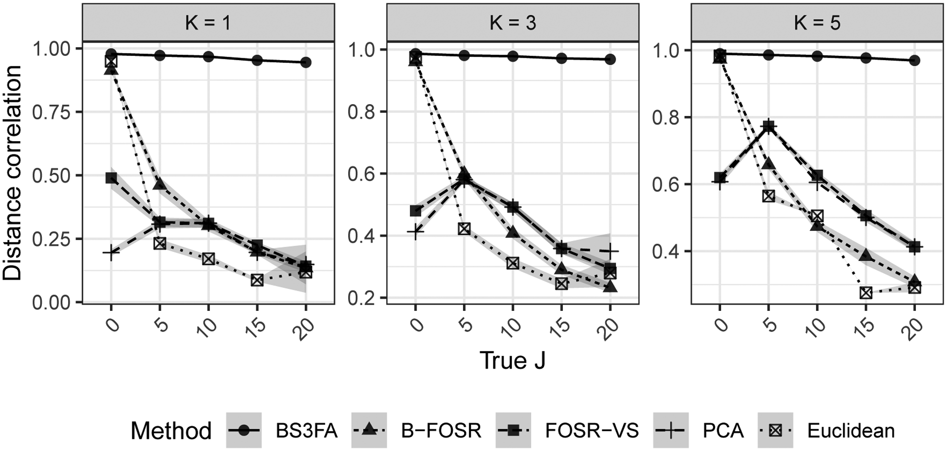
Correlation between entries in the true pairwise distance matrix (i.e., the Euclidean distance between true latent factors η) and the predicted pairwise distance matrix for holdout chemicals. Each subplot shows the result of 100 simulations per J across methods for a given true shared subspace dimension K.

Figure 10 shows the mean squared predictive error (MSPE) for the simulated hold-out chemicals’ dose-response mean functions. Although the performance of all models deteriorates as the amount of “superfluous” information in X increases (i.e., as J increases), the BS³FA and B-FOSR models are the most robust, showing superior performance across all values of K and J. The BS³FA consistently outperforms the B-FOSR model, with MSPE of the latter on average 1.5 times higher than that of the former (the 95% quantile of this multiplicative factor ranges from 1.1 to 2.4 across all simulations and values of K and J). The BAABTP model appears most sensitive to the value of J, with MSPE near that of BS³FA model when J is small, but among the worst MSPE when J is high. The LASSO model is able to perform fairly well when K is small, but, as K increases, it is unable to learn the more complicated relationship between x_i and y_i. The FOSR-VS model becomes increasingly sensitive to J as K increases.

Fig. 10.

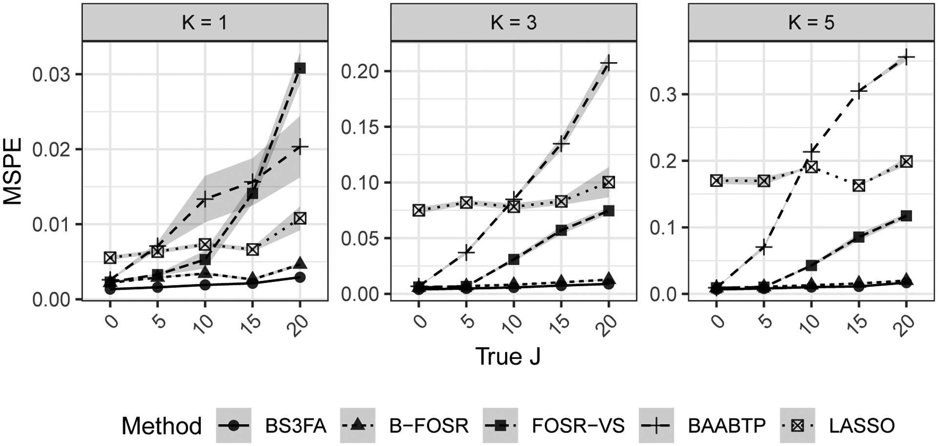
Mean squared predictive error (MSPE) for the hold-out chemicals’ dose-response mean functions. Each subplot shows the result of 100 simulations per J across methods for a given true shared subspace dimension K.

Coverage of the simultaneous bands for the BS³FA model remains close to nominal across all values of K and J. Additionally, these band widths are narrowest subject to (at least) nominal coverage across competitors and for all values of K and J. The coverage of the BAABTP model is consistently below nominal and decreases as J increases, another reflection of its overall poor predictive performance. The coverage of the B-FOSR model is much higher than nominal, nearing 1 across all values of K and J, and the simultaneous bands are wider on average than those of BS³FA. Detailed results for both coverage and band width are available in the Supplementary Material (Moran et al. (2021)).

In the ToxCast analysis following this section, we discuss results from one possible method of deeming a chemical active. Namely, call a chemical active if its global Bayesian p-value (Meyer et al. (2015)) is less than 0.05. The null hypothesis in this case is that the dose-response mean function equals 0 everywhere, that is, that a chemical is inactive. If alternatively activation (suppression) is of specific interest, one could use the additional requirement that the direction of observed effect be positive (negative) in order to reject the null. The true positive rate (TPR), false positive rate (FPR) and false discovery rate (FDR) of this method on the simulated data are shown in Table 1. Across all values of K and J, the TPR is generally high, and the FPR and FDR are near zero. Note that the TPR increases with K and decreases with J, while FPR and FDR remain stable across values of K and J. That is, the model seems more likely to identify chemicals as active, as the dimension of the latent toxicity-relevant space increases, but loses sensitivity when there is more toxicity-irrelevant information. Results for the B-FOSR method, provided in the Supplementary Material (Moran et al. (2021)), show slightly improved TPRs but at the cost of much higher FPRs and FDRs (whereas for BS³FA the FPR and FDR are consistently near zero, these values range from 0.1 to 0.5 across K and J for B-FOSR).

Table 1.

True positive rate (TPR), false positive rate (FPR) and false discovery rate (FDR) for the proposed method of assessing whether a chemical is active. A perfect classifier has a TPR of 1 and an FPR/FDR of 0. Shown is the mean (SD) across simulations

		J = 0	J = 5	J = 10	J = 15	J = 20
TPR	K = 1	0.72 (0.08)	0.66 (0.08)	0.64 (0.07)	0.58 (0.06)	0.52 (0.09)
	K = 3	0.98 (0.03)	0.97 (0.03)	0.97 (0.03)	0.95 (0.04)	0.93 (0.05)
	K = 5	1.00 (0.01)	1.00 (0.01)	1.00 (0.01)	0.99 (0.01)	0.98 (0.02)
FPR	K = 1	0.00 (0.00)	0.00 (0.00)	0.00 (0.01)	0.00 (0.00)	0.00 (0.00)
	K = 3	0.00 (0.01)	0.00 (0.01)	0.00 (0.01)	0.00 (0.01)	0.00 (0.01)
	K = 5	0.00 (0.01)	0.00 (0.01)	0.00 (0.01)	0.00 (0.01)	0.00 (0.01)
FDR	K = 1	0.00 (0.01)	0.00 (0.01)	0.00 (0.01)	0.00 (0.00)	0.00 (0.01)
	K = 3	0.00 (0.01)	0.00 (0.01)	0.00 (0.01)	0.00 (0.01)	0.00 (0.01)
	K = 5	0.00 (0.01)	0.00 (0.01)	0.00 (0.01)	0.00 (0.01)	0.00 (0.01)

When there is misalignment between the structure assumed by the BS³FA model and the true data generating process, BS³FA is still able to predict similarly to or better than the competitors. As with the well-aligned simulation, BS³FA is robust to increasing “superfluous” information in X. A similar story can be seen in the coverage and distance results for the misaligned simulation. Even when the assumed latent factor model is not the model from which data are simulated, the coverage of BS³FA is close to nominal. B-FOSR, on the other hand, suffers from much higher than nominal coverage across all simulations while BAABTP suffers from much lower than nominal coverage as “superfluous” information in X increases. BS³FA is still able to recover a distance metric that is highly correlated (mean correlation 0.97, range 0.94 to 0.99 across simulations) with the distance in the true relevant X dimensions, although B-FOSR more perfectly learns such a metric. Visual results are shown in the Supplementary Material (Moran et al. (2021)).

4. Relating chemical structure to toxicological response.

Data preprocessing steps and results of the analysis of the ToxCast ATG PXR assay are discussed in the following subsections. The structure of BS³FA allows for learning about structured variability in both the feature and response space, prioritizing chemicals for future evaluation, and predicting chemical activity for as yet unobserved chemicals.

4.1. ToxCast setup.

Observations below the cytotoxicity limit for 3,540 Phase 1, Phase 2 and e1k chemicals tested in the AttaGene PXR assay are included in our data analysis. The structure information for each chemical is summarized by 777 Mold2 chemical features (Hong et al. (2008)). As discussed previously, BS³FA has the advantage of being able to effectively ignore toxicity-irrelevant features via shrinkage on elements of Θ, making the careful curation of a feature set unnecessary.

Chemicals having no provided SMILES information (n = 405) were omitted from further analysis. The result is 3,135 chemicals having Mold2 descriptions of their chemical structure. Note that some chemicals have identical Mold2 output. These sets of chemicals are, in effect, considered a single chemical (i.e., treated as multiply observed dose-response curves by the model). For analysis the number of “unique” chemical sets (i.e., the number of unique SMILES represented across the 3,135 chemicals) is N = 3,070. The eight most common dose concentrations are −1.05, −0.52, −0.1, 0.3, 0.85, 1.3, 1.85, 2.3 log uM (see the vertical white bands in Figure 11), but BS³FA allows both common and unique doses. As the bulk of chemicals have no information about extremely low (< −2 log uM) dose activity (see Figure 11), the data considered are the D = 38 unique doses ≥ −2 log uM, out of the 56 total unique doses. Approximately 4% of chemicals have multiple observed dose-response curves, for example, Allethrin and Clorophene from Figure 2. While such repeated measurements may come from different experimental runs, unfortunately the data set does not provide information on which point is associated with which run, so we assume independence in this respect rather than, for example, adding a run-specific random effect term.

Mold2 is used to generate a set of 777 numeric molecular descriptors associated with each chemical. As noted above, some chemicals exactly shared these descriptors due to Mold2’s inability to capture certain differentiating structures (see the Supplementary Material (Moran et al. (2021)) for an example); these “identical” chemicals were treated as multiple observed chemicals. After removing features having no variability (99 total, including, e.g., features equalling zero for all chemicals, such as number of 11-membered rings and number of Argon), features with duplicated entries (16) or features having > 99% of chemicals sharing a feature value (99, e.g., only one chemical has any aromatic group urea derivatives), S = 563 features remain. As a further preprocessing step, the continuous variables are scaled to have mean 0 and variance 1. Further information on creating and using Mold2 descriptors is included in the Supplementary Material (Moran et al. (2021)).

In order to mimic the scenario of using the BS³FA model to prioritize chemicals for further screening, we hold out all of the dose-response observations for 25% of chemicals in the data set. That is, we provide the model with these chemicals’ structure but not their dose-response curves. Of interest will be how similar these unobserved chemicals are to known active chemicals and the AC50 (the dose at 50% of maximum activity) for unobserved chemicals predicted by the model to be activity-increasing. Recall for the purpose of this analysis, we consider a chemical activity-increasing if the global Bayesian p-value (Meyer et al. (2015)) of its dose-response profile is less than 0.05 and the direction of observed effect is positive.

A global mean term μ^y is included in the model (see Figure 12) to account for a nonzero average profile rather than mean centering, as the low number of observations at less common doses leads to a “noisy” center. Additionally, the dose-response matrix is scaled by a multiplicative factor so that the scaled X and Y matrices have the same Frobenius norm (a measure of total variation); specifically, set $Y=\parallel X{\parallel }_F\frac{Y}{\parallel Y{\parallel }_F}$. This rescaling keeps larger matrices from dominating when learning the shared column-specific shrinkage terms {τ_k} or the shared score vectors {η_i} (e.g., when S is much larger than D, as in this setting).

Fig. 12.

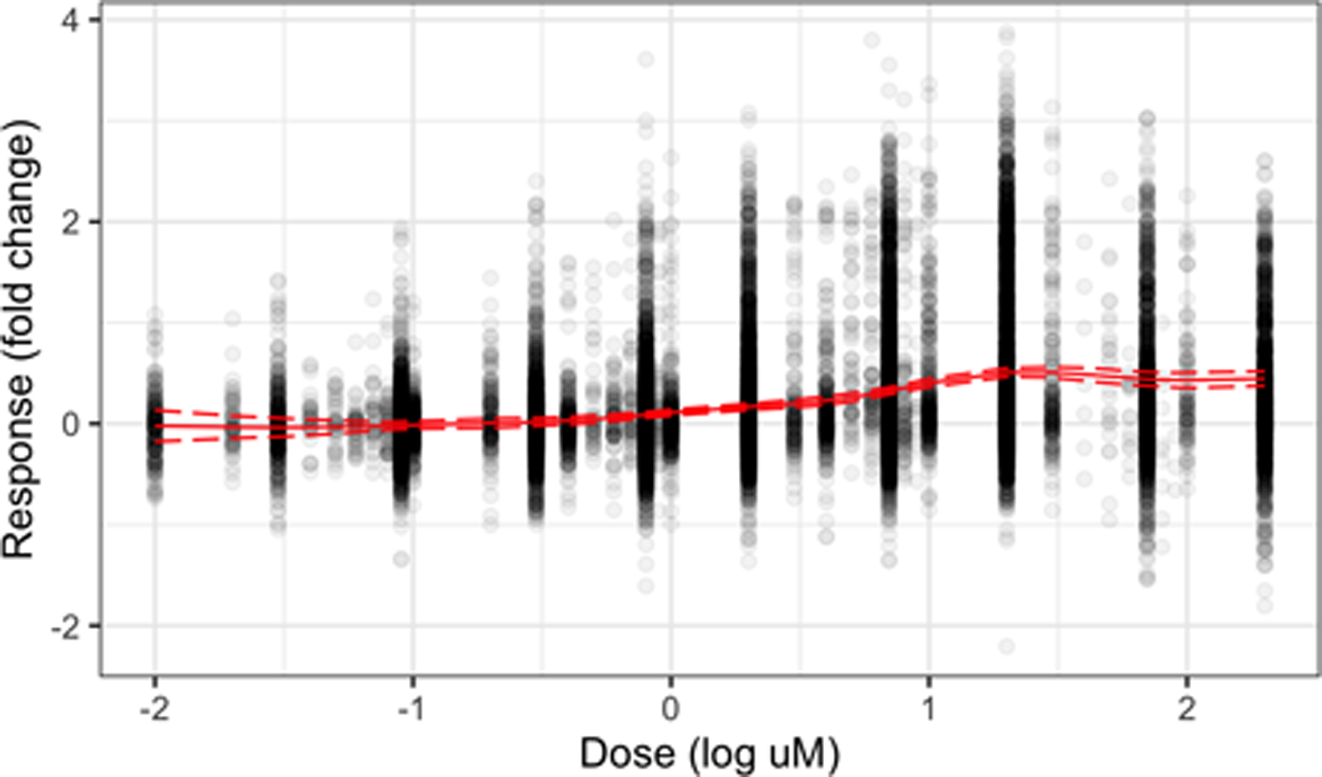
All response values at each dose in the data set. The solid line shows the model-predicted global mean μ^y and the dashed lines show the model-predicted 95% simultaneous credible band about μ^y.

We ran the sampler for 40,000 iterations. After an initial burn-in of 20,000 iterations, every 10th sample was saved. Computation time was approximately eight hours on a 2016 Mac-Book pro with a 2.9 GHz Intel Core i7 processor. Trace plots of model predictions show good mixing; these, along with those of model components and an assessment of the sufficiency of the chosen K and J values, are available in the Supplementary Material (Moran et al. (2021)).

4.2. Model components.

The learned matrix Λ, shown on the left side of Figure 13, provides a snapshot of the directions of structured variation present in the dose-response data. The first column of Λ, shown in the top middle of Figure 13, is the dominant factor loading (i.e., the factor loading having the largest estimated norm). Unsurprisingly, this vector takes the shape of a prototypical dose-response curve. Later columns of Λ act to provide smooth deviations from this prototypical shape. For example, the third column characterizes a flat profile until around −1 log uM followed by a near-linear increase until leveling off at a dose value just under 2 log uM, while the fourth column shows an initial start point above zero followed by a gentle U-shaped dip.

Fig. 13.

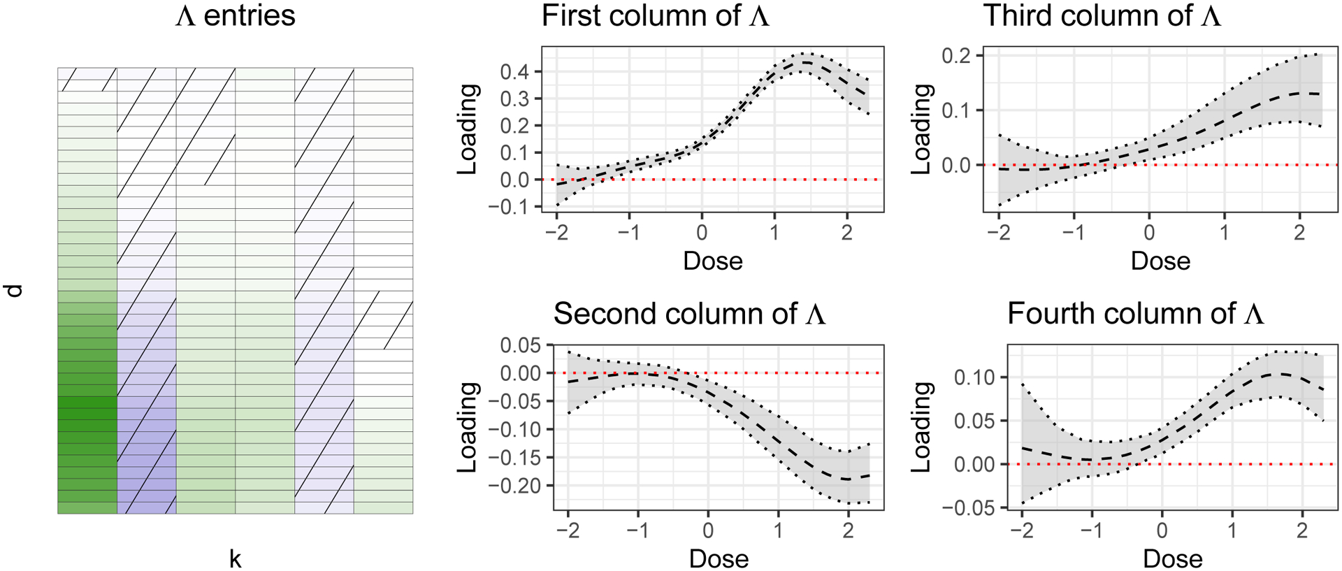
Left: First six columns of the predicted mean of Λ. Each row represents a unique dose value. Middle and right: Mean and 95% simultaneous bands for the first four columns of Λ. The dose values are given on the x-axis.

The learned matrix Θ, the values of which are shown in Figure 14, provides a snapshot of the directions of structured toxicity-relevant variation present in the feature data. The bulk of the estimated entries are very close to 0 due to the shrinkage effect of the horseshoe prior. The BS³FA model structure allows us to interpret the nonzero entries of a given column of Θ as being those related to the particular structure present in the corresponding column of Λ. For example, the significantly nonzero entries of the first column of Θ are those associated with the prototypical activity profile seen in the top row of the middle column of Figure 13. By absolute magnitude the largest such features include the number of group esters, the number of group X-C on aromatic ring, the sum of the topological distance between the vertices O and Cl, the number of Chlorine and the sum eigenvalue weighted by polarizability distance matrix.

FIG. 14.

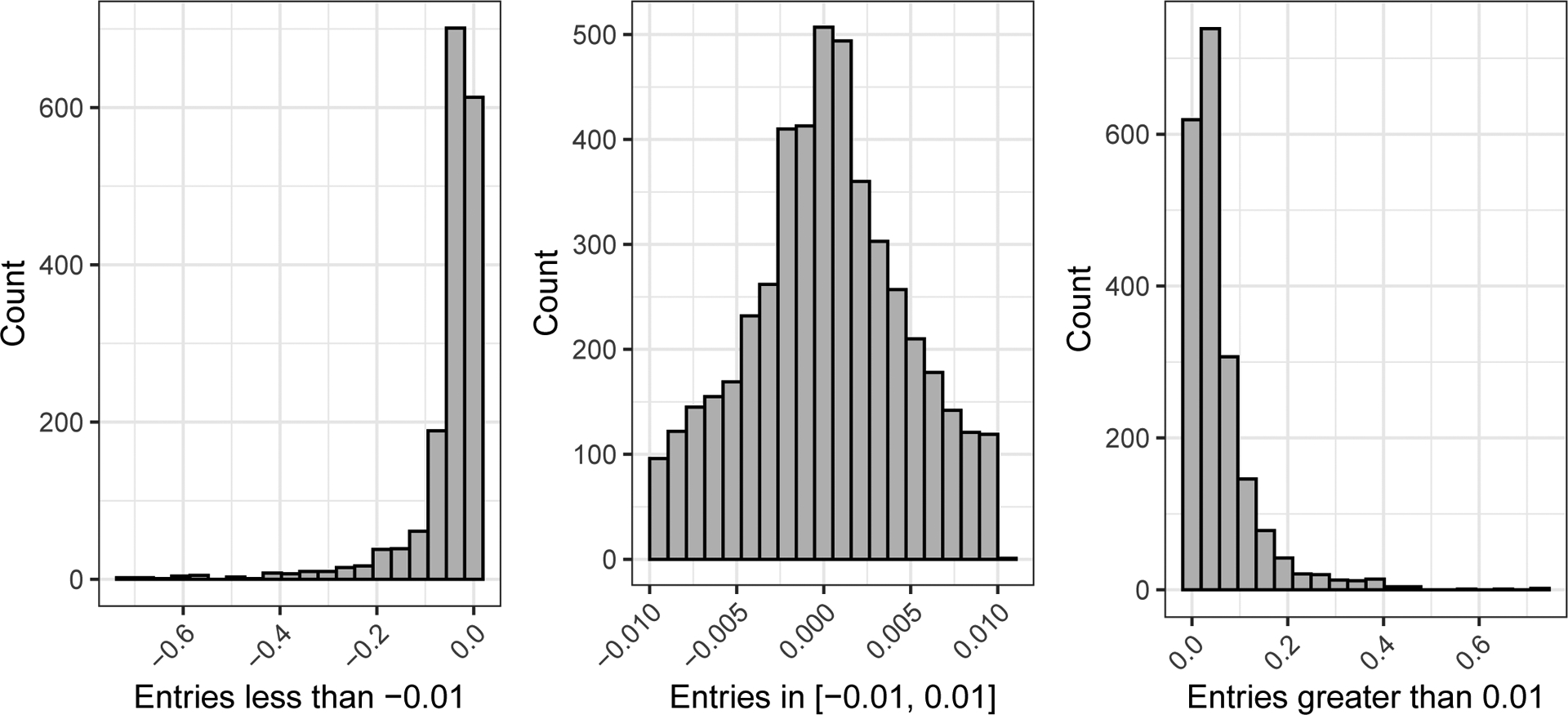
Histogram showing entries of the predicted mean of Θ. The bulk of the estimated entries are close to 0 due to the shrinkage effect of the horseshoe prior.

The chemicals having extreme positive values of η₁ will be those for which the dose-response profile has a large component due to λ₁ and a large chunk of toxicity-relevant molecular variability described by the first column of Θ. In the training set the chemicals having the largest expected value for η₁ are Calcium bromide, Nickel(II) chloride, Dibromomethane, Zinc chloride, and Dimethylamine. All are known toxins. Several of these chemicals have in common the presence of Cl, so it is unsurprising that features involving Cl appeared amongst the high-value loadings components for the first column of Θ.

4.3. Distance learning.

Figure 15 shows the predicted pairwise distance matrix between a set of example chemicals chosen as clusters of chemicals in the training set closest to specific recognizable hold-out chemicals. Included are a cluster of similar low-activity chemicals (the training chemicals nearest to hold-out chemical Saccharin) in the bottom left block and a cluster of similar high-activity chemicals (the training chemicals nearest to hold-out chemical Clomiphene citrate (1:1)) in the central block. A handful of miscellaneous chemicals that are fairly isolated in η space relative to the other included chemicals are shown in the top-right block.

Fig. 15.

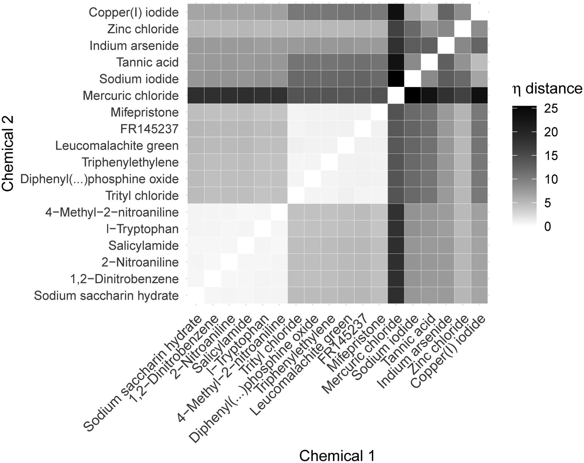
Expected distance in η space for a select set of training chemicals.

When selecting future chemicals for prioritization, one can either seek to “fill in” the space around chemicals of known toxicity relevance or to “venture out” into spaces not near any currently tested chemicals. While addressing this experimental design problem is outside the scope of this work, we assume for the sake of exposition that both possible avenues are of interest. We further assume that the set of hold-out chemicals represents the space of options for further in vitro testing.

Assuming the central cluster of chemicals in Figure 15 is of interest for more targeted exploration, we could select the hold-out chemicals closest to that set to test further. In terms of average distance between each cluster member, the four closest chemicals in the hold-out set are Clomiphene citrate (1:1) (i.e., our “seed” chemical for this training group for which the model predictive performance can be seen in Figure 17), 4-Hydroxytamoxifen, Tamoxifen, and Tamoxifen citrate. Research has suggested similarity in action between Clomiphene citrate and Tamoxifen (Dhaliwal et al. (2011), Seyedoshohadaei, Zandvakily and Shahgeibi (2012)), lending credence to this distance measure’s accounting of activity-relevant similarity.

Fig. 17.

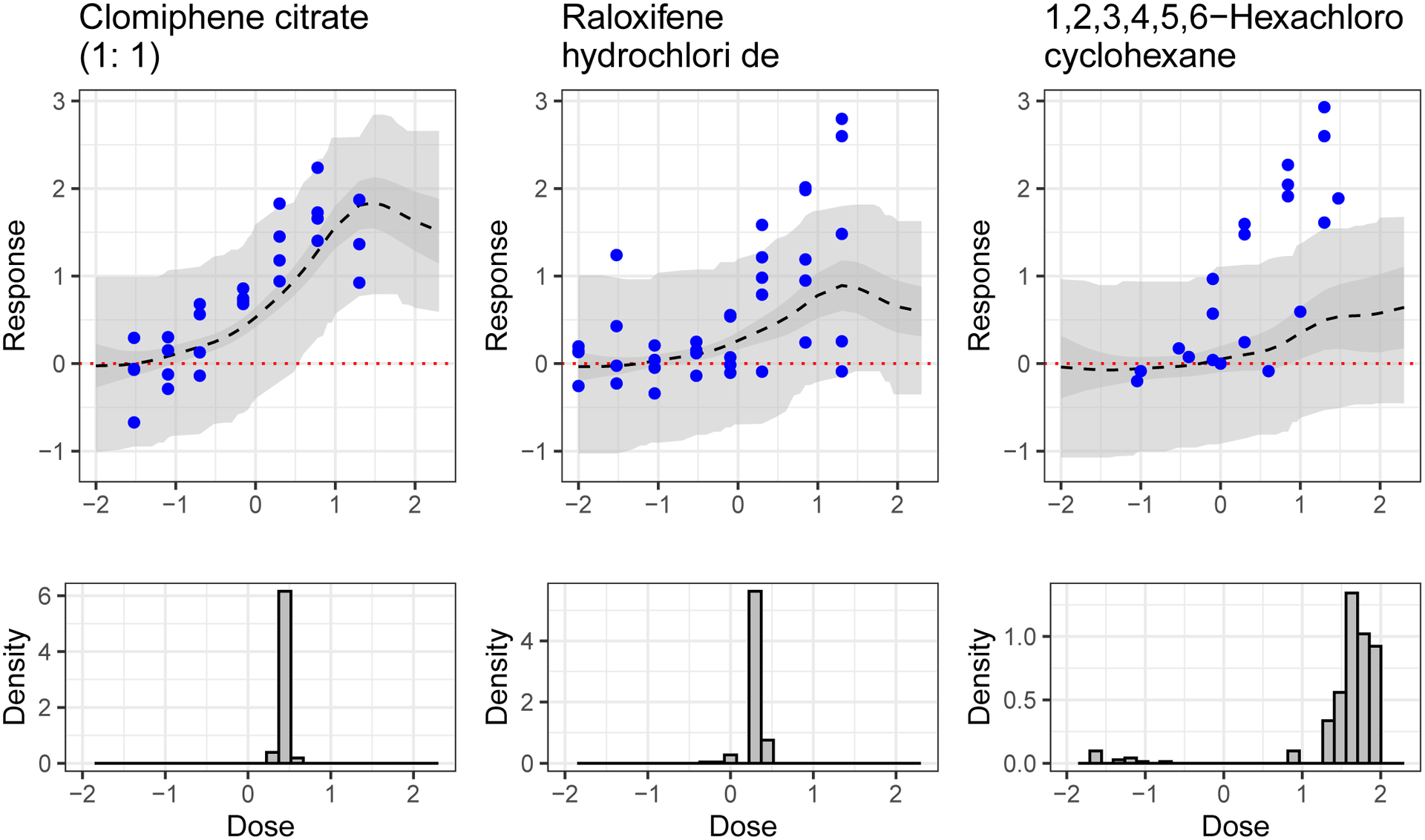
Results for heavily tested hold-out chemicals predicted by the model to be activating. MSEs from left to right are 0.21, 0.49 and 1.44. Top: Predicted average dose-response curve (dashed black line), 95% simultaneous band for expected dose-response curve (darker grey ribbon) and 95% simultaneous band for observed data (lighter grey ribbon). Data (held out in training) are solid points. Bottom: Posterior samples of the AC50 value, that is, the dose at which the dose-response curve is at half of its maximal value.

If, on the other hand, our goal was to test new chemicals that are least similar to observed chemicals, then we could choose the hold-out chemicals having the largest minimum distance to a training chemical. Assuming we chose such chemicals iteratively, we would select Tetracosafluorotetradecahydrophenanthrene (a solvent used in the preparation of certain polymers), Strychnine hemisulphate salt (a pesticide used for rodent and bird control), and Cadmium dinitrate (a colorant and photographic flash powder component). That these chemicals are the most distant in η space from both the training set and each other suggests that the model considers them to have distinctive activity relevant variability. See Figure 16 for their structure diagrams; the predicted activity for Cadmium dinitrate is also shown in Figure 18.

Fig. 16.

From left to right: Tetracosafluorotetradecahydrophenanthrene, Strychnine hemisulphate salt and Cadmium dinitrate.

Fig. 18.

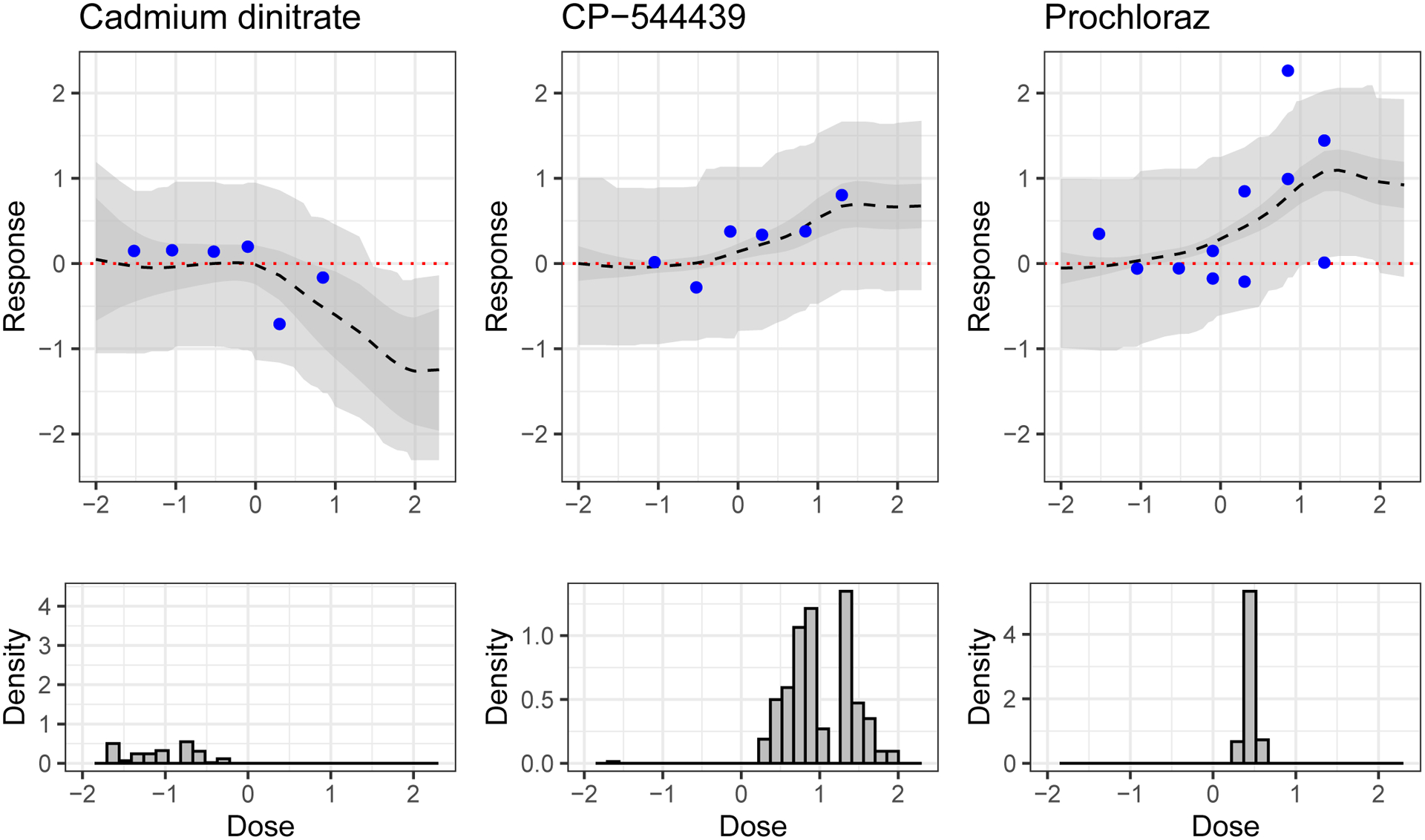
Results for hold-out chemicals predicted by the model to be active (activity decreasing in the case of Cadmium dinitrate). MSEs from left to right are 0.10, 0.03 and 0.40. Top: Predicted average dose-response curve (dashed black line), 95% simultaneous band for expected dose-response curve (darker grey ribbon) and 95% simultaneous band for observed data (lighter grey ribbon). Data (held out in training) are solid points. Bottom: Posterior samples of the AC50 value, that is, the dose at which the dose-response curve is at half of its maximal value.

4.4. Prediction.

Overall, the MSE between the data and the predicted dose-response profiles is 0.24 for the training chemicals and 0.30 for the hold-out chemicals. For comparison, the straw man model using the mean of the training data at a given dose to predict the hold-out data at that dose leads to an MSE of 0.37 and predicting all hold-out dose-response profiles to be inactive (i.e., 0 everywhere) yields an MSE of 0.47. LASSO using dose, feature and the interaction between dose and feature gives an MSE of 0.31 for the training chemicals and 0.40 for the hold-out chemicals. The B-FOSR model, as run using the fosr() function in the fosr package, had unstable predictions, as the amount of missingness in the training data was too high (recall Figure 11) for the imputation scheme used in the code—the MSE was in the 100s. Limiting the training data to only include the most commonly observed dose levels did not resolve this issue. The fosr.vs() function simply returned an error due to the amount of missingness in the training data. The BAABTP model was not run for the toxicity data for computation time reasons.

The 95% prediction intervals for the BS³FA model run cover 94.2% of the training data and 92.6% of the hold-out data, respectively. Unsurprisingly, hold-out chemicals having lower coverage also tend to have higher MSE. The coverage for specific hold-out chemicals is inversely related to the minimum distance between that chemical and its closest neighboring training chemical, while the MSE is directly related to the minimum distance between that chemical and its closest neighboring training chemical. That is, as a hold-out chemical moves farther away from other training chemicals, on average its coverage and MSE become worse. This finding suggests that increasing the amount of training data with specific care to the lesser-known regions of the chemical feature space would likely improve the model’s MSE and coverage.

We say a chemical is predicted to be activating, that is, to increase activity, if the global Bayesian p-value (Meyer et al. (2015)) for the predicted dose-response profile is less than 0.05 and the 95% simultaneous bands exceed 0 for at least one dose value. Figures 17 and 18 show model-predicted mean dose-response (MDR) curves along with samples of the AC50 value, that is, the dose at which the dose-response curve is at half of its maximal value, for activating hold-out chemicals. The predicted mean and 95% posterior bands for the MDR curves are smooth due to the underlying structure of Λ. The proportion of hold-out chemicals deemed activating by our model is nearly twice as high among the population of chemicals that are heavily tested (i.e., that have 10 or more observations). Since chemicals that are known to have toxic effects tend to be more heavily tested, this finding is suggestive of the model’s capability to detect activity.

Although the predictive ability of the model is imperfect (e.g., 1, 2, 3, 4, 5, 6-Hexachloro-cyclohexane in Figure 17 is under-predicted), overall performance appears reasonable. Particularly poorly predicted chemicals, examples of which are shown in the Supplementary Material (Moran et al. (2021)), tend to have shapes that differ from the common profiles and/or be farther in η space from training data than well-predicted curves. Also note that, although the observations above the reported cytotoxicity limit were removed prior to running the model, the hormesis shape (i.e., the downturn at the end of the predicted dose-response profile) remains prominent in highly active chemicals, because it is a feature of the first column of Λ, which has the highest column norm and drives large scale variation across profiles.

In the context of this experiment, we fail to reject the null hypothesis that a chemical is inactive if its global Bayesian p-value (Meyer et al. (2015)) is greater than 0.05 (i.e., if the bounds of the 95% posterior simultaneous bands for the predicted MDR curve include zero at all points). For convenience, we refer to these chemicals as being predicted to be inactive by the model. Figure 19 shows model-predicted inactive dose-response curves for hold-out chemicals. As before, the predictions are smooth and appear reasonable relative to the true data. On average, hold-out chemicals deemed inactive under the criteria outlined above have a lower true maximum observed response than those deemed activity-increasing.

Fig. 19.

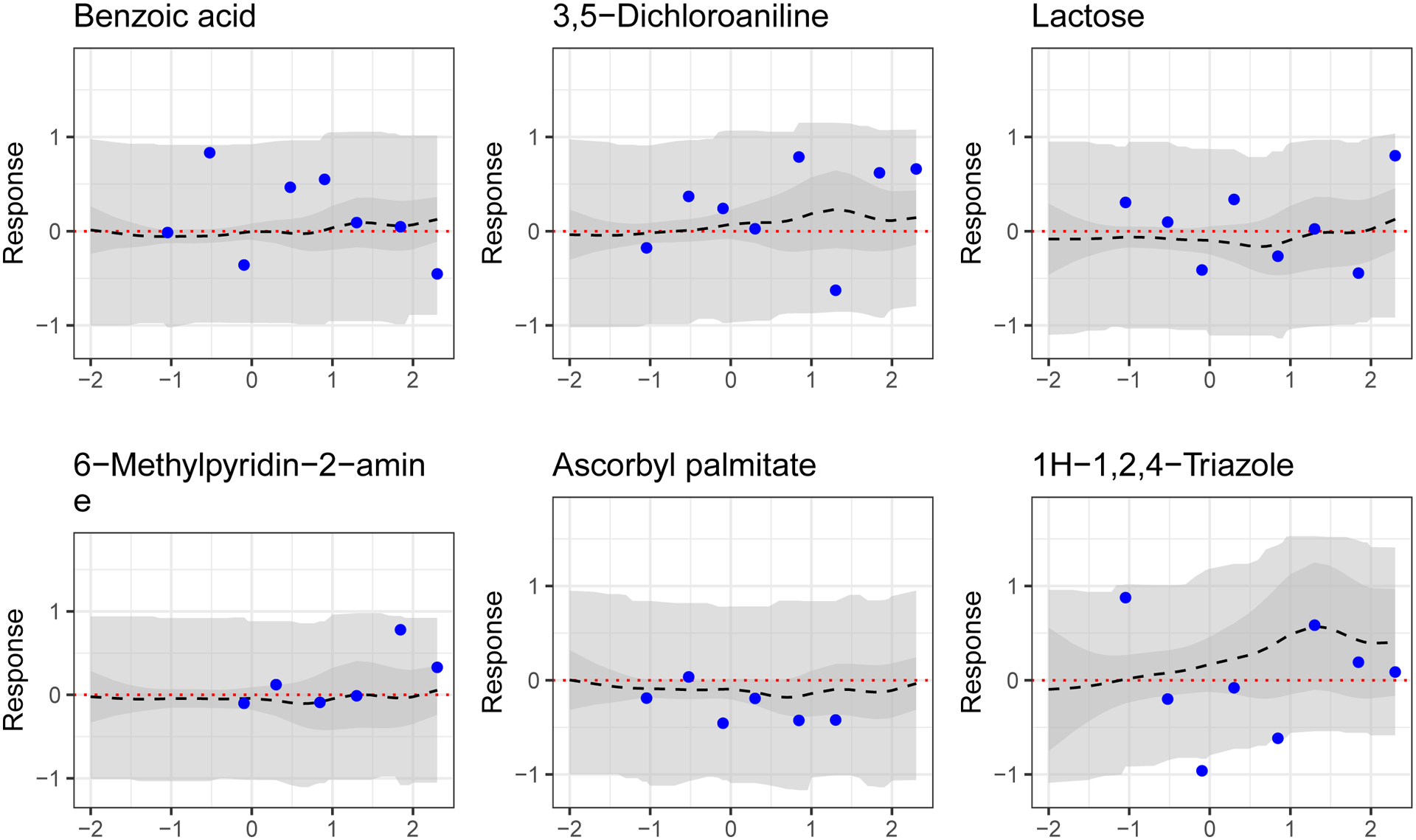
Results for select hold-out chemicals predicted by the model to be inactive. MSEs from left to right, top to bottom, are 0.22, 0.23, 0.14, 0.13, 0.06 and 0.42. Shown are predicted average dose-response curve (dashed black line), 95% simultaneous band for expected dose-response curve (darker grey ribbon) and 95% simultaneous band for observed data (lighter grey ribbon). Data (held out in training) are solid points.

The choice of how to prioritize chemicals for future evaluation is flexible. Assuming there are in fact no dose-response data for the hold-out chemicals, a simple scheme by which chemicals could be selected for in vitro study, based on their BS³FA predictions, would be to screen all chemicals for which the lower limit of the 1 − α posterior simultaneous bands for the MDR curve exceeds some threshold (e.g., 0). The value of α could be selected with attention to the resources available, a larger α would lead to more chemicals being screened, whereas a smaller α would mean only those chemicals the model is most confident about would be screened. Once the set of chemicals are selected for further testing, the order of screening could be determined by chemicals’ expected AC50 value, by the maximum value of their predicted MDR curves, by the highest value taken by the lower α/2 simultaneous band for expected response, by their proximity in latent space to known toxic chemicals, or by another metric of interest.

For example, if one chooses α = 0.05, then 68% of hold-out chemicals have predicted dose-response curve lower bound that at some point exceeds 0. The five highest priority chemicals using the max lower bound method would be Basic Blue 7, Ergocalciferol, Toremifene citrate, 4-(2-Phenylpropan-2-yl)-N-[4-(2-phenylpropan-2-yl)phenyl]aniline, and 2,4-Bis(1-methyl-1-phenylethyl)phenol. As discussed previously, Toremifene citrate is a close relative of Clomiphene citrate (1:1) (activity shown in Figure 17) and a selective estrogen receptor modulator used to treat ovulatory dysfunction in women trying to become pregnant. Basic Blue 7 is labeled as corrosive, an irritant, acutely toxic, and an environmental hazard. The closest neighbors to Basic Blue 7 in the training set are other colorants, Gentian Violet and Malachite green, that have known toxic effects (Docampo and Moreno (1990), Srivastava, Sinha and Roy (2004)).

5. Conclusion.

We have focused on the utility of distance learning for designing future chemical test sets, but these pairwise distance matrices could be used in place of Euclidean distance in any distance-based statistical analysis. This would include distance-based clustering of chemicals as well as kernel and Gaussian process-based models. As a specific example the authors believe these activity-relevant distances have the potential to improve main effects estimates in mixture models for human health outcomes. It is likely that incorporating knowledge about similarity in activity-relevant space (e.g., by using the toxicity-relevant pairwise distance matrix to inform a group penalized regression model) would provide stabilization for main effects and, in turn, allow for better estimation of the interaction effects.

The designation of active vs. inactive in the BS³FA model is based on a posterior summary of the predicted dose-response profiles; there is no direct incorporation of the concept of a chemical being inactive in the model itself. It may be desirable, particularly when considering assays having very few chemicals presenting with any activity, to probabilistically model inactivity. For example, the dose-response profile could be modeled as a mixture between the zero-vector and the BS³FA factor model with a learned weight on the zero vector corresponding to the probability of inactivity.

The BS³FA model deals with the structured decomposition of a single assay and a single feature data set. In reality, any sort of model hoping to extend to human health outcomes will need to utilize information from multiple sources. In the ToxCast data set, there is not just one dose-response curve per chemical. There are many assay endpoints of potential relevance to human toxicity. Furthermore, there are potentially many useful chemical feature descriptors (we used Mold2, but others include MACCS keys, Daylight Fingerprints, or Morgan Fingerprints, to name a few). Future work will link the ideas in BS³FA to those in Wilson, Reif and Reich (2014) to allow for a more direct active/inactive assignation and to hierarchically describe variability across multiple assays. Extending even further, the holy grail of toxicity modeling would be an explicit linking of multiple assay endpoints to human health data such that human health outcomes could be predicted from chemical structure alone.

REFERENCES

- Barber RF, Reimherr M and Schill T (2017). The function-on-scalar LASSO with applications to longitudinal GWAS. Electron. J. Stat 11 1351–1389. MR3635916 10.1214/17-EJS1260 [DOI] [Google Scholar]
- Bhattacharya A and Dunson DB (2011). Sparse Bayesian infinite factor models. Biometrika 98 291–306. MR2806429 10.1093/biomet/asr013 [DOI] [PMC free article] [PubMed] [Google Scholar]
- Canale A and Dunson DB (2013). Nonparametric Bayes modelling of count processes. Biometrika 100 801–816. MR3142333 10.1093/biomet/ast037 [DOI] [Google Scholar]
- Carvalho CM, Polson NG and Scott JG (2010). The horseshoe estimator for sparse signals. Biometrika 97 465–480. MR2650751 10.1093/biomet/asq017 [DOI] [Google Scholar]
- Chen Y, Goldsmith J and Ogden RT (2016). Variable selection in function-on-scalar regression. Stat 5 88–101. MR3478799 10.1002/sta4.106 [DOI] [PMC free article] [PubMed] [Google Scholar]
- Dhaliwal LK, Suri V, Gupta KR and Sahdev S (2011). Tamoxifen: An alternative to clomiphene in women with polycystic ovary syndrome. Journal of Human Reproductive Sciences 4 76. [DOI] [PMC free article] [PubMed] [Google Scholar]
- Dix DJ, Houck KA, Martin MT, Richard AM, Setzer RW and Kavlock RJ (2007). The ToxCast program for prioritizing toxicity testing of environmental chemicals. Toxicol. Sci 95 5–12. 10.1093/toxsci/kfl103 [DOI] [PubMed] [Google Scholar]
- Docampo R and Moreno SN (1990). The metabolism and mode of action of gentian violet. Drug Metab. Rev 22 161–178. [DOI] [PubMed] [Google Scholar]
- Durante D (2017). A note on the multiplicative gamma process. Statist. Probab. Lett 122 198–204. MR3584158 10.1016/j.spl.2016.11.014 [DOI] [Google Scholar]
- Fan Z and Reimherr M (2017). High-dimensional adaptive function-on-scalar regression. Econom. Stat 1 167–183. MR3669995 10.1016/j.ecosta.2016.08.001 [DOI] [Google Scholar]
- Hahn PR and Carvalho CM (2015). Decoupling shrinkage and selection in Bayesian linear models: A posterior summary perspective. J. Amer. Statist. Assoc 110 435–448. MR3338514 10.1080/01621459.2014.993077 [DOI] [Google Scholar]
- Hong H, Xie Q, Ge W, Qian F, Fang H, Shi L, Su Z, Perkins R and Tong W (2008). Mold2, molecular descriptors from 2D structures for chemoinformatics and toxicoinformatics. J. Chem. Inf. Model 48 1337–1344. [DOI] [PubMed] [Google Scholar]
- Hong H, Slavov S, Ge W, Qian F, Su Z, Fang H, Cheng Y, Perkins R, Shi L et al. (2012). Mold2 molecular descriptors for QSAR. In Statistical Modelling of Molecular Descriptors in QSAR/QSPR 2 65–109. [Google Scholar]
- Judson RS, Houck KA, Kavlock RJ, Knudsen TB, Martin MT, Mortensen HM, Reif DM, Rotroff DM, Shah I et al. (2009). In vitro screening of environmental chemicals for targeted testing prioritization: The ToxCast project. Environ. Health Perspect 118 485–492. [DOI] [PMC free article] [PubMed] [Google Scholar]
- Kavlock R, Chandler K, Houck K, Hunter S, Judson R, Kleinstreuer N, Knudsen T, Martin M, Padilla S et al. (2012). Update on EPA’s ToxCast program: Providing high throughput decision support tools for chemical risk management. Chem. Res. Toxicol 25 1287–1302. [DOI] [PubMed] [Google Scholar]
- Kliewer SA, Goodwin B and Willson TM (2002). The nuclear pregnane X receptor: A key regulator of xenobiotic metabolism. Endocr. Rev 23 687–702. 10.1210/er.2001-0038 [DOI] [PubMed] [Google Scholar]
- Knowles D and Ghahramani Z (2011). Nonparametric Bayesian sparse factor models with application to gene expression modeling. Ann. Appl. Stat 5 1534–1552. MR2849785 10.1214/10-AOAS435 [DOI] [Google Scholar]
- Kowal DR and Bourgeois DC (2020). Bayesian function-on-scalars regression for high-dimensional data. J. Comput. Graph. Statist 29 629–638. MR4153187 10.1080/10618600.2019.1710837 [DOI] [Google Scholar]
- Li G, Shen H and Huang JZ (2016). Supervised sparse and functional principal component analysis. J. Comput. Graph. Statist 25 859–878. MR3533642 10.1080/10618600.2015.1064434 [DOI] [Google Scholar]
- Liu R, Rallo R, George S, Ji Z, Nair S, Nel AE and Cohen Y (2011). Classification NanoSAR development for cytotoxicity of metal oxide nanoparticles. Small 7 1118–1126. [DOI] [PMC free article] [PubMed] [Google Scholar]
- Lock EF, Hoadley KA, Marron JS and NOBEL AB (2013). Joint and individual variation explained (JIVE) for integrated analysis of multiple data types. Ann. Appl. Stat 7 523–542. MR3086429 10.1214/12-AOAS597 [DOI] [PMC free article] [PubMed] [Google Scholar]
- Low-Kam C, Telesca D, Ji Z, Zhang H, Xia T, Zink JI and Nel AE (2015). A Bayesian regression tree approach to identify the effect of nanoparticles’ properties on toxicity profiles. Ann. Appl. Stat 9 383–401. MR3341120 10.1214/14-AOAS797 [DOI] [Google Scholar]
- Makalic E and Schmidt DF (2016). A simple sampler for the horseshoe estimator. IEEE Signal Process. Lett 23 179–182. [Google Scholar]
- Martin YC, Kofron JL and Traphagen LM (2002). Do structurally similar molecules have similar biological activity? J. of Med. Chem 45 4350–4358. [DOI] [PubMed] [Google Scholar]
- Meng J, Zhang J, Qi Y, Chen Y and Huang Y (2010). Uncovering transcriptional regulatory networks by sparse Bayesian factor model. EURASIP J. Adv. Signal Process 2010 3. [Google Scholar]
- Meyer MJ, Coull BA, Versace F, Cinciripini P and Morris JS (2015). Bayesian function-on-function regression for multilevel functional data. Biometrics 71 563–574. MR3402592 10.1111/biom.12299 [DOI] [PMC free article] [PubMed] [Google Scholar]
- Montagna S, Tokdar ST, Neelon B and Dunson DB (2012). Bayesian latent factor regression for functional and longitudinal data. Biometrics 68 1064–1073. MR3040013 10.1111/j.1541-0420.2012.01788.x [DOI] [PMC free article] [PubMed] [Google Scholar]
- Moran KR, Dunson D, Wheeler MW and Herring AH (2021). Supplement to “Bayesian joint modeling of chemical structure and dose response curves.” https://doi.org/10.1214/21-AOAS1461SUPPA, https://doi.org/10.1214/21-AOAS1461SUPPB, https://doi.org/10.1214/21-AOAS1461SUPPC [DOI] [PMC free article] [PubMed] [Google Scholar]
- Nikolova N and Jaworska J (2003). Approaches to measure chemical similarity—a review. QSAR & Combinatorial Science 22 1006–1026. [Google Scholar]
- O’connell MJ and Lock EF (2019). Linked matrix factorization. Biometrics 75 582–592. MR3999181 10.1111/biom.13010 [DOI] [PubMed] [Google Scholar]
- Patel T, Telesca D, Low-Kam C, Ji ZX, Zhang HY, Xia T, Zinc JI and Nel AE (2014). Relating nano-particle properties to biological outcomes in exposure escalation experiments. Environmetrics 25 57–68. MR3233744 10.1002/env.2246 [DOI] [PMC free article] [PubMed] [Google Scholar]
- Pati D, Bhattacharya A, Pillai NS and Dunson D (2014). Posterior contraction in sparse Bayesian factor models for massive covariance matrices. Ann. Statist 42 1102–1130. MR3210997 10.1214/14-AOS1215 [DOI] [Google Scholar]
- Ray P, Zheng L, Lucas J and Carin L (2014). Bayesian joint analysis of heterogeneous genomics data. Bioinformatics 30 1370–1376. [DOI] [PubMed] [Google Scholar]
- Seyedoshohadaei F, Zandvakily F and Shahgeibi S (2012). Comparison of the effectiveness of clomiphene citrate, tamoxifen and letrozole in ovulation induction in infertility due to isolated unovulation. Iran. J. Reprod. Med 10 531–536. [PMC free article] [PubMed] [Google Scholar]
- Srivastava S, Sinha R and Roy D (2004). Toxicological effects of malachite green. Aquat. Toxicol 66 319–329. [DOI] [PubMed] [Google Scholar]
- Weininger D (1988). SMILES, a chemical language and information system. 1. Introduction to methodology and encoding rules. J. Chem. Inf. Comput. Sci 28 31–36. [Google Scholar]
- Wheeler MW (2019). Bayesian additive adaptive basis tensor product models for modeling high dimensional surfaces: An application to high-throughput toxicity testing. Biometrics 75 193–201. MR3953720 [DOI] [PMC free article] [PubMed] [Google Scholar]
- Wilson A, Reif DM and Reich BJ (2014). Hierarchical dose-response modeling for high-throughput toxicity screening of environmental chemicals. Biometrics 70 237–246. MR3251684 10.1111/biom.12114 [DOI] [PubMed] [Google Scholar]
- Yoshida R and West M (2010). Bayesian learning in sparse graphical factor models via variational mean-field annealing. J. Mach. Learn. Res 11 1771–1798. MR2653356 [PMC free article] [PubMed] [Google Scholar]
Associated Data
This section collects any data citations, data availability statements, or supplementary materials included in this article.