Depthgram: Visualizing outliers in high‐dimensional functional data with application to fMRI data exploration

Abstract

Functional magnetic resonance imaging (fMRI) is a non‐invasive technique that facilitates the study of brain activity by measuring changes in blood flow. Brain activity signals can be recorded during the alternate performance of given tasks, that is, task fMRI (tfMRI), or during resting‐state, that is, resting‐state fMRI (rsfMRI), as a measure of baseline brain activity. This contributes to the understanding of how the human brain is organized in functionally distinct subdivisions. fMRI experiments from high‐resolution scans provide hundred of thousands of longitudinal signals for each individual, corresponding to brain activity measurements over each voxel of the brain along the duration of the experiment. In this context, we propose novel visualization techniques for high‐dimensional functional data relying on depth‐based notions that enable computationally efficient 2‐dim representations of fMRI data, which elucidate sample composition, outlier presence, and individual variability. We believe that this previous step is crucial to any inferential approach willing to identify neuroscientific patterns across individuals, tasks, and brain regions. We present the proposed technique via an extensive simulation study, and demonstrate its application on a motor and language tfMRI experiment.

1. INTRODUCTION

Functional magnetic resonance imaging (fMRI) is the benchmark neuroimaging technique for measuring brain activity, owing its advantages over other acquisition methods, such as PET or EEG. In fact, it is non‐invasive and does not involve radiation, which makes it safe for the subject. In addition, it provides optimal spatial and temporal resolution (finer for the spatial component). fMRI based on blood‐oxygen‐level dependent (BOLD) involves measuring the variation on oxygen consumption and blood flow that occur in brain regions in response to neural activity, which enables the identification of regions that participate in specific mental processes. Task fMRI (tfMRI) experiments are conducted by measuring brain activity in this manner for a given period of time (several minutes) while the subject is asked to repeatedly perform some task, alternating between task performance and resting periods for the entire length of the experiment. On the other hand, resting‐state fMRI (rsfMRI) experiments allow to record brain activity during periods of rest. These experiments are often conducted on a relatively small group of patients (approximately a hundred at most) because of cost constraints and other feasibility reasons. However, there exist recent initiatives of large multi‐site databases such as the UK Biobank ¹ or the ABCD study. ² In any case, the dataset obtained for each one of the subjects is significantly large, owing to the high spatial resolution of the technique. Refer to Reference ³ for a detailed description of this type of experiments, including tasks specification for tfMRI.

The analysis of fMRI data poses different challenges. Zhang et al ⁴ enumerate some of them in the context of an attempt to characterize task‐based and resting state fMRI signals. Among them, we focus on: (1) the high inter‐individual variability in a setting where the number of individuals is relatively small; (2) the high amount of available data for a single experiment, owing to the voxel‐wise structure of fMRI temporal signals; and (3) the existence of different sources of noise, from individual origins (movement during the experiment, lack of attention, etc.) to mechanical nature (scanner instability among others), that induce artifacts and undesirable measurement values in the recorded signals.

In this setting, data visualization and outlier detection tools are crucial to avoid feeding inferential algorithms with low‐quality data. In fact, in any context in which high‐dimensionality or complex data structure does not allow for the direct visual inspection of data, the application of visualization tools in low dimension and robust measures help elucidate sample composition. In particular, for functional data, of which fMRI data can be a particular case, a substantial amount of studies exist on robust visualization and outlier detection tools based on depth‐measures (see, for instance, References 5 and 6).

In functional data analysis (FDA), individual observations are real functions over a given domain, usually accounting for time, observed at discrete points. If several functions over the same domain are observed for each individual, we refer to multivariate FDA. In this setting, the number p of functions observed per individual is small, relative to the number n of individuals. Examples of this include the longitudinal patterns of flying, feeding, walking, and resting observed over the lifespan of Drosophila flies, ⁷ or the 8‐variate signal of electrocardiograph curves. ⁸

Regarding fMRI data, multiple functions of time are observed on each individual, corresponding to the recorded brain activity on each voxel over the duration of the experiment. However, the number of dimensions is given by the number of voxels which, depending on the resolution of the scan, can be in the order of hundred of thousands, while the number of individuals is relatively small, owing to cost and time constraints. Nevertheless, the access to large multi‐site databases, such as UK Biobank ¹ or ABCD study, ² is increasingly common. As visual checking of data quality is particularly difficult on these large datasets, automatic pre‐identification of possible outliers might be of special interest here too. In any case, a new paradigm is emerging in multivariate FDA with small to moderately large n and very large p, which we refer to as the high‐dimensional functional data setting. Several proposals exist in the literature for the analysis of this type of data, based on dimensionality reduction. They primarily rely on multivariate functional principal component analysis ^{9 , 10} that facilitates the extraction of main features of the data for inferential purposes. In this work, we primarily consider a previous stage of analysis, focusing on data exploration and anomaly detection.

The literature on robust multivariate functional data mainly relies on the concept of depth for visualization and outlier detection. However, some very recent non‐depth based approaches ¹¹ also address these questions. In the case of generalizing functional depth to the multivariate functional setting, two main directions have been adopted. One of the first approaches was proposed by Ieva and Paganoni ⁸ who defined a multivariate functional depth measure as a weighted sum of the functional band depths ¹² computed over marginal functional datasets. Later, Claeskens et al ¹³ proposed a different definition comprising the integration over the time domain of any multivariate depth measure computed on the p‐dimensional sample of points observed at each time instant. Based on these definitions, several visualization tools have been proposed to enable data inspection and detection of outlying observations. On one hand, Ieva and Paganoni ¹⁴ extended the outliergram ⁶ to the multivariate framework for component‐wise outlier detection. On the other hand, given an integrated multivariate functional depth measure or its outlyingness counterpart, several visualization tools have been defined as a two‐dimensional graphical representation of its average value (over the time domain) vs some measure of its variability (also over time). This allows us to distinguish typical observations (low depth/outlyingness variability over time) from magnitude (low average depth, resp. high average outlyingness) and shape (high depth/outlyingness variability) outliers. Examples of these include the centrality‐stability plot (CS‐plot) of Reference ¹⁵ and its modification proposed by Nieto‐Reyes and Cuesta‐Albertos. ¹⁶ Recently, two new approaches followed this same direction based on different directional outlyingness notions that are computationally more efficient than the existing alternatives, and proposed corresponding graphical representations, the functional outlier map (FOM) ¹⁷ and magnitude‐shape plot (MS‐plot). ¹⁸ These approaches both offer interesting results in the low‐dimensional multivariate functional setting.

In this study, we consider a different approach. We propose a methodology for reducing the high‐dimensional functional problem to a functional problem by maintaining, and not averaging, depth values over dimensions (voxels) and time. The use of computationally efficient depth‐based measures allows us to achieve this, even for very large p. The analysis of the resulting functional datasets, namely depths over dimensions and time, elucidates sample composition and outlier presence. In particular, we focus on the identification of joint outliers, because marginal outliers can be detected via standard functional data techniques applied on each dimension. A graphical 2D representation of the data, the Depthgram, is also proposed.

The remainder of this article is presented as follows. In Section 2, we discuss the taxonomy of atypical observations in multivariate and high‐dimensional functional datasets, and introduce the proposed depth‐based visualization techniques, providing the properties of the functional depth measures that form the basis for the methodology. In Section 3, we verify the performance of our visualization tools via a simulation study in the high‐dimensional setting, and assess its computational efficiency in comparison with existing methods for low multivariate functional data. In Section 4, we demonstrate the application of the proposed approach with a motor and language tfMRI experiment conducted on 100 individuals. Finally, we conclude the article with a discussion presented in Section 5.

2. VISUALIZATION OF HIGH‐DIMENSIONAL FUNCTIONAL DATA

A general setting in FDA considers that observations are i.i.d. realizations of some stochastic process $\mathbf{X}$, taking values in the space of continuous functions defined from some compact real interval $ℐ$ into ${ℝ}^p$, $𝒞(ℐ,{ℝ}^p)$. In other words, a sample of size n of functional data is a collection of n i.i.d. continuous functions $X_i:ℐ\to {ℝ}^p$, $i=1,\dots ,n$, whose realizations $x_i(t)$, $t\in ℐ$, are observed on a time grid of N points, $\{t_1,\dots ,t_N\}\subseteq ℐ$. We denote $x_i^j:ℐ\to ℝ$ as the jth component of the ith observation. If $p=1$, we are in the univariate functional data setting, where each individual has associated a curve, whereas if $p>1$ we are in the multivariate functional data setting, where for each individual we observe several processes over time. In this work, we consider the case $p\gg n$, and refer to it as the high‐dimensional functional data setting. In particular, in the context of fMRI experiments, n is generally in the order $10^2$ to $10^3$, while p is in the order $10^5$ to $10^6$.

2.1. Outliers in multivariate and high‐dimensional functional data

In FDA, outlying observations are generally classified as magnitude outliers, curves with values lying outside the range of the majority of the data, or shape outliers, curves that exhibit a shape that differs from the rest of the sample. Magnitude outliers are also referred to as shift outliers, and some times, the distinction between isolated and persistent outliers, is considered. Refer to References 15 and 19 for a detailed taxonomy of functional outliers. All these notions apply to a set of observed curves over the same time interval, that is, to univariate functional data. In the multivariate FDA framework, we need to consider a higher hierarchy to distinguish between marginal and joint outliers. Marginal outliers would be observations whose marginal components fall in some of the above mentioned categories, in one or several dimensions, while joint outliers would be observations with non‐outlying marginals, but joint outlying behavior. In fact, when thinking of fMRI data, we can imagine individuals for which brain activity patterns are standard in every voxel, with atypical relationships across brain regions. Figure 1 illustrates the outlier categorization in a bivariate synthetic dataset.

FIGURE 1.

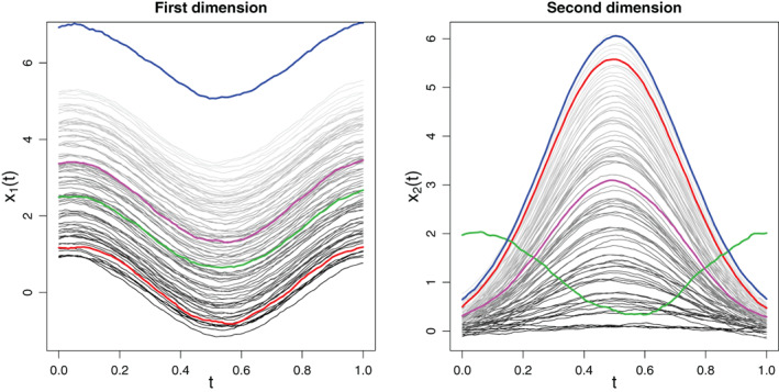
Bivariate functional sample where the same color is adopted to draw both components of an observation. High values in the first component tend to correspond to high values in the second component. Three outlying observations are highlighted: A marginal shape outlier in the second dimension (green), a marginal magnitude outlier in the first dimension (blue), and a joint outlier (red). For the red observation, low values in the first dimension are associated with high values in the second dimension, although none of its marginals is outlying in any of the dimensions. The magenta curve represents a central observation

Therefore, the outlier detection for multivariate functional data needs to rely on procedures that can jointly detect outliers over dimensions, and not solely marginally. The depth‐based methods proposed in the literature to define population depth/outlyingness measures for multivariate functional data primarily rely on two approaches (notice also the existence of some non‐depth‐based approaches ¹¹ ): (1) given a functional depth measure, define a multivariate functional depth measure by averaging it over dimensions, as proposed in Reference ⁸; and (2) given a multivariate depth measure, define a multivariate functional depth measure by integrating it over the time domain. Outlier detection methods based on depth measures or their outlyingness counterparts defined under the second approach will be able to identify joint outliers, as soon as they rely on depth (outlyingness) measures for multivariate data that are designed to do so in finite dimensional spaces. This is the case for some recent approaches, as References 15, 16, 17, 18. However, in general, multivariate depth functions are computationally expensive, or even unfeasible for moderate dimension, ²⁰ and efficient alternatives such as the random Tukey depth (as in Reference ¹⁶) or the directional outlyingness of Reference ¹⁷ may fail to provide a computationally efficient method in a high‐dimensional functional setting (refer to Section 3.2). To address this situation, we propose to work with highly efficient depth notions based on the concept of band depth refer to Reference ²¹, that apply to both functional and multivariate spaces. Moreover, instead of considering any of the two approaches described above, we embrace the depth of depths approach, which enables us to better characterize different types of observations and outlying behaviors.

2.2. Depth‐based tools for high‐dimensional functional data

We now present some depth notions for functional data that will be incorporated into our procedure. Let us recall the modified band depth (MBD) and modified epigraph index (MEI), a depth measure and depth‐based index defined for the analysis of functional data in References 12 and 22, respectively. Subsequently, their sample versions are provided. Let $x_1,\dots ,x_n$ be n continuous functions defined on a given compact real interval $ℐ$. For any $x\in \{x_1,\dots ,x_n\}$,

$$MB{D}_{\{x_1,\dots ,x_n\}}(x)={\left(\genfrac{}{}{0ex}{}{n}{2}\right)}^{-1}{\displaystyle \sum _{i=1}^n}{\displaystyle \sum _{j=i+1}^n}{\displaystyle \frac{\lambda \left(\left\{t\in ℐ|\min (x_i(t),x_j(t))\le x(t)\le \max (x_i(t),x_j(t))\right\}\right)}{\lambda (ℐ)}},$$

$$ME{I}_{\{x_1,\dots ,x_n\}}(x)={\displaystyle \frac{1}{n}}{\displaystyle \sum _{i=1}^n}{\displaystyle \frac{\lambda \left(\left\{t\in ℐ|x_i(t)\ge x(t)\right\}\right)}{\lambda (ℐ)}},$$

where $\lambda (·)$ stands for the Lebesgue measure on $ℝ$. $MBD$ represents the average, over all possible pairs of curves, of the proportion of time that a curve spends in the band defined by any two curves in the sample. $MEI$ represents the mean proportion of time that a curve lies below the curves of the sample.

In Reference ⁶, a quadratic relationship between these two quantities was established which enabled the definition of a procedure to detect shape outliers. Indeed, in a univariate functional dataset, a curve can exhibit a low MBD value because it has an atypical shape or because it has a typical shape, but is far from the center of the bulk of curves or both. However, a curve can only obtain a high MBD value if it is central in both shape and location. Therefore, because the MBD of a curve is highly dependent on its location in the sample (in the sense of vertical position), and the MEI provides a measure of this location, the conditional observation of the MBD given the MEI provides an accurate shape descriptor, which allows the identification of shape outliers, that is, curves with low MBD values for relatively high MEI values. In particular it was proved that

$$MB{D}_{\{x_1,\dots ,x_n\}}(x)\le f_n\left(ME{I}_{\{x_1,\dots ,x_n\}}(x)\right),x\in \{x_1,\dots ,x_n\},$$ (1)

where $f_n:[0,1]\to ℝ$ is the parabola defined by $f_n(z)=a_0+a_{1}z+a_2{n}^2{z}^2$ and $a_0=a_2=-2/n(n-1)$, $a_1=2(n+1)/(n-1)$ (notice the dependence on the sample size). The equality in (1) holds, if and only if none of the curves in the sample cross each other.

Let us introduce some notation in the context of multivariate functional data. Given a sample $\mathbf{x}=\{x_i={(x_i^j(t_k))}_{k=1,\dots ,N}^{j=1,\dots ,p},i=1,\dots ,n\}$ of p‐variate functions observed at discrete time points, we will consider the $n\times p$ matrix ${\mathbf{MBD}}_d(\mathbf{x})$ whose $ij$ element corresponds to the modified band depth of curve $x_i^j$ relative to the jth marginal sample, that is, ${\mathbf{MBD}}_d{(\mathbf{x})}_{ij}=MB{D}_{\{x_1^j,\dots ,x_n^j\}}(x_i^j)$. The subindex d of ${\mathbf{MBD}}_d(\mathbf{x})$ represents dimensions, meaning that the MBD is computed on each dimension of the dataset. Indeed, the columns of ${\mathbf{MBD}}_d(\mathbf{x})$ are the MBDs on each marginal. Equivalently, we will denote ${\mathbf{MEI}}_d(\mathbf{x})$, the $n\times p$ matrix whose columns are the MEIs on each marginal of the sample, that is, ${\mathbf{MEI}}_d{(\mathbf{x})}_{ij}=ME{I}_{\{x_1^j,\dots ,x_n^j\}}(x_i^j)$, $i=1,\dots ,n$, $j=1,\dots ,p$.

Similarly, we will denote by ${\mathbf{MBD}}_t(\mathbf{x})$, the $n\times N$ matrix whose columns are the MBDs on each time point of the sample, and ${\mathbf{MEI}}_t(\mathbf{x})$ (dimension $n\times N$).

Now, each one of these four matrices can be understood as a set of functional observations, indexed by dimensions or time. In other words, MBD and MEI (or other depth functions) can be computed on them as will be discussed in the next section.

2.3. Relationship between MEI(MBD) and MBD(MEI)

In a functional univariate setting, the most central individuals according to the modified band depth correspond to the overall highest values of $MBD$ while the most central individuals according to the modified epigraph index correspond to the overall most central values (close to 0.5) of $MEI$, and both quantities are related by Equation (1).

When switching to the multivariate functional framework, one would expect that individuals that are persistently central over dimensions according to $MBD$, will exhibit an $MBD$ curve (row) in the matrix ${\mathbf{MBD}}_d(\mathbf{x})$ with higher values than most of the rest of the individuals. In contrast, individuals that are persistently far from the center of the sample across dimensions in the $MBD$ sense would exhibit a low $MBD$ curve (row) in the matrix ${\mathbf{MBD}}_d(\mathbf{x})$. In other words, if we apply the modified epigraph index on the $MBD$ sample, we should obtain low values for the central individuals and high values for the non‐central individuals. Now, if we consider the $MEI$ matrix ${\mathbf{MEI}}_d(\mathbf{x})$, observations with central values across dimensions will exhibit a central curve in the matrix, while individuals whose corresponding curves take low or high values across dimensions, will tend to exhibit high and low $MEI$ curves in ${\mathbf{MEI}}_d(\mathbf{x})$. Again, if we now apply the modified band depth on the $MEI$ sample, we should obtain high $MBD$ values for those individuals with curves that take central values in every dimension.

This expected behavior is summarized in the following result, whose proof is provided under Supplementary Materials.

Proposition 1

Let

$\mathbf{x}=\{x_i={(x_i^j(t_k))}_{k=1,\dots ,N}^{j=1,\dots ,p},i=1,\dots ,n\}$

be a sample of p‐variate continuous functions observed at N discrete time points. If

• (a)
  $(x_i^j(t_{k_1})-x_h^j(t_{k_1}))(x_i^j(t_{k_2})-x_h^j(t_{k_2}))>0$

  ,

  $k_1,k_2\in 1,\dots ,N$

  ,

  $i\ne h$

  , for all

  $j=1,\dots ,p$

  then

$$MBD\left({\mathbf{MEI}}_d(x)\right)\le g_n\left(1-MEI\left({\mathbf{MBD}}_d(x)\right)\right),x\in \{x_1,\dots ,x_n\},$$ (2)

where

$g_n:[0,1]\to ℝ$

,

$g_n(z)={\alpha }_0+z+{\alpha }_2{z}^2$

, with

${\alpha }_0=2/n$

,

${\alpha }_2=-n/2(n-1)$

. Moreover, if

• (b)
  $(x_i^j(t_k)-x_h^j(t_k))(x_i^{\ell }(t_k)-x_h^{\ell }(t_k))>0$

  ,

  $k=1,\dots ,N$

  ,

  $i\ne h$

  ,

  $j\ne \ell$

  also holds, then

$$MBD\left({\mathbf{MEI}}_d(x)\right)=g_n\left(1-MEI\left({\mathbf{MBD}}_d(x)\right)\right),x\in \{x_1,\dots ,x_n\},$$ (3)

with $g_n$ as in a).

Remark 1

Assumptions (a) and (b) will not hold in practice, as they require a perfectly ordered set of curves inside each dimension and across dimensions. However, Proposition 1 establishes the theoretical relationship between the two measures of interest, thereby justifying their combination.

Remark 2

The results of Proposition 1 also hold for $MBD\left({\mathbf{MEI}}_t(x)\right)$ and $MEI\left({\mathbf{MBD}}_t(x)\right)$ under the same assumptions (in reverse order), and the proof follows the same lines.

The 2D representation of $1-MEI({\mathbf{MBD}}_d(\mathbf{x}))$ and $MBD({\mathbf{MEI}}_d(\mathbf{x}))$ enable the identification of different types of observations. Refer to Figure 2 for an example. Note that we adopt $1-MEI$ and not $MEI$ in the x‐axis, such that for both axes high and low values indicate central and non‐central observations, respectively. In this representation, the most central observations will appear in the right top corner, while the least central observations will be presented in the left bottom corner. This includes magnitude outliers, which will be found at the left bottom corner of the plot, but not necessarily isolated from the data cloud (as it is also the case in the outliergram). Shape outliers will tend to appear in the left upper part of the graphic, above a bulk of the majority of sample points.

FIGURE 2.

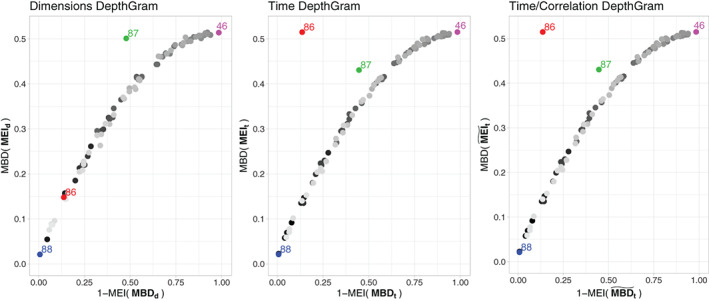
Two‐dimensional representations of the bivariate sample of Figure 1. Left: Depths over dimensions. Center: Depths over time points. Right: Depths for time/correlation correction (Section 2.4). The most central observation is found at the right top corner in the plots. The joint outlier is isolated in the time plot, while the shape outlier is isolated in the dimensions plot

Let us now consider the representation of $1-MEI({\mathbf{MBD}}_t(\mathbf{x}))$ vs $MBD({\mathbf{MEI}}_t(\mathbf{x}))$. The interpretation of extreme values in both axes is similar to the previous one; however, in this case joint outliers function as shape outliers. Certainly, joint outliers are observations that have an association pattern across dimensions (shape when the functional data is considered as a function of dimensions for a fixed time point) that differs from that of the majority of the observations.

In fact, this only holds if the association across dimensions is positive, that is, the ordering of the curves is preserved from one dimension to the next one. Otherwise, the identification of an observation whose components exhibit a different association behavior is not straightforward, as illustrated in Figure 3. Note that in this case, we consider ${\mathbf{x}}_i(t)=(x_i^1(t),\dots ,x_i^p(t))$ as a functional observation, and we apply functional depth tools on it. In such a setting, multivariate depth tools would be more beneficial in detecting joint outliers at each time point. Another complex situation is the case where an observation exhibits a clear association pattern across its components, and the rest of the observations are independent dimension‐wise. However, in this case, conventional multivariate depths applied marginally on the observations for each time point will also fail. This is illustrated in Figure 4.

FIGURE 3.

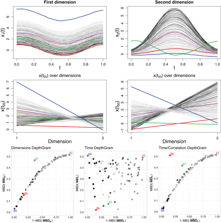
First row: A bivariate functional dataset with reversed curve ordering between the two dimensions. Second row: Bivariate observations for $t_{20}=0.2$ and $t_{50}=0.5$, represented using a parallel coordinate plot (the choice of time points is arbitrary and is adopted for illustration). Third row: DepthGrams. The same color is used across the figures to identify individual observations. The observation coded in red is a joint outlier, because low values in the first dimension are associated with low values in the second dimension, where the opposite holds for the rest of the curves in the sample. Because there are changes in the sign of the correlation among dimensions, the third Depthgram version is most suitable for identifying joint outliers

FIGURE 4.

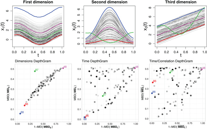
First row: A three‐variate functional dataset with independent components. Second row: DepthGrams. The same color is used across the figures to identify individual observations. The observation depicted in red could be considered as a joint outlier, because low values in the first dimension are associated with low values in the second and third dimensions, while the rest of the curves behave independently across dimensions. The same is true for the blue observation, which, in addition, is a magnitude outlier in the first dimension. There is a spurious negative correlation between the second and third components of the dataset; hence, the time/correlation Depthgram differs from the time Depthgram. However, because no clear correlation pattern is present in the sample, both exhibit the same dispersed appearance

2.4. DepthGrams

We propose three graphical representations of the data based on the relationships between $MEI$ of $MBD$ and $MBD$ of $MEI$ as already detailed. On one hand, the DepthGram on dimensions, where functional depths are first computed on the sample of curves $x_{1:n}^j$ observed over $\{t_1,\dots ,t_N\}$, for each $j=1,\dots ,p$, and the DepthGram on time, where functional depths are first computed on the sample of p‐dimensional observations $x_{1:n}(t_k)$, for each time point $k=1,\dots ,N$. On the other hand, the time/correlation DepthGram, which is just the time DepthGram on a modified dataset, to correct for negative association across dimensions.

• Dimensions DepthGram: Scatter plot of points $D{G}_i^d=(D{G}_{i1}^d,D{G}_{i2}^d)=$ $\left(1-MEI({\mathbf{MBD}}_d{(\mathbf{x})}_{i•}),\right.$ $\left.MBD({\mathbf{MEI}}_d{(\mathbf{x})}_{i•})\right)$, $i=1,\dots ,n$.

• Time DepthGram: Scatter plot of points $D{G}_i^t=(D{G}_{i1}^t,D{G}_{i2}^t)=$ $\left(1-MEI({\mathbf{MBD}}_t{(\mathbf{x})}_{i•}),\right.$ $\left.MBD({\mathbf{MEI}}_t{(\mathbf{x})}_{i•})\right)$, $i=1,\dots ,n$.

• Time/Correlation DepthGram: Scatter plot of points $D{G}_i^{tc}=(D{G}_{i1}^{tc},D{G}_{i2}^{tc})=$ $\left(1-MEI({\mathbf{MBD}}_t{(\tilde{\mathbf{x}})}_{i•}),\right.$ $\left.MBD({\mathbf{MEI}}_t{(\tilde{\mathbf{x}})}_{i•})\right)$, $i=1,\dots ,n$, with ${\tilde{x}}_i^j(t)=x_i^j(t){\prod }_{k=2}^{j}sign(\rho ({\mathbf{MEI}}_d{(\mathbf{x})}_{•k-1},{\mathbf{MEI}}_d{(\mathbf{x})}_{•k}))$, $i=1,\dots ,n$, where $\rho (·,·)$ denotes Pearson's correlation coefficient function.

The motivation for this third representation is the possible presence of negative association between some of the dimensions, as illustrated in Figure 3. The underlying idea is to define a new sample $\tilde{\mathbf{x}}$ with the same structure on the marginals and positive association between dimensions. This association is quantified as the linear correlation between curve ranks (in terms of $MEI$). Certainly, at each dimension j, $j=1,\dots ,p$, ${\tilde{x}}_i^j$ is equal to $x_i^j$, except for a possible change in sign that reverses the order of the curves. The procedure starts at $j=2$, where for $i=1,\dots ,n$, ${\tilde{x}}_i^2$ is defined as $-x_i^2$ if the correlation between ${\mathbf{MEI}}_d{(\mathbf{x})}_{•\hspace{0.17em}2}$ and ${\mathbf{MEI}}_d{(\mathbf{x})}_{•\hspace{0.17em}1}$ is negative, and ${\tilde{x}}_i^2=x_i^2$ otherwise. For $j>2$, ${\tilde{x}}_i^j=-x_i^j$, if the correlation between ${\mathbf{MEI}}_d{(\mathbf{x})}_{•\hspace{0.17em}j}$ and ${\mathbf{MEI}}_d{(\tilde{\mathbf{x}})}_{•j-1}$ is negative, and ${\tilde{x}}_i^j=x_i^j$ otherwise. Accordingly, because the relative shape and position of the curves are preserved inside each component of the sample, depths computed marginally on each dimension (those used to build the Dimension DepthGram) would be the same. However, because the transformed sample $\tilde{\mathbf{x}}$ has a positive association pattern along dimensions, the time DepthGram computed on it will differ from that built on $\mathbf{x}$ because at any time point, multivariate observations will tend to have a more regular behavior for most of the observations, and joint outliers will stand out in the parallel coordinate representation of these multivariate samples.

Unlike other existing tools based on outlyingness measures, the DepthGram representations are bounded in both horizontal ($MEI$ of $MBD$s) and vertical ($MBD$ of $MEI$s) axes, which eases interpretation. In fact, it is not just a tool for the visual identification of outliers, but also for the two‐dimensional representation of the entire sample, which also allows us to visualize central individuals and sample variability on time and dimensions. Although the result of Proposition 1 establishes the conceptual basis for the definition of an outlier detection rule, as atypical observations will tend to lie above the parabola $g_n$, the determination of a threshold for this rule requires the approximation of the distribution of the distances to the parabola, which is unfeasible in the high‐dimensional setting considered in this study (refer to Section 3.2 for an approximate non‐optimized detection rule). However, the fact that scales are fixed on both axes of the DepthGram plots and that outliers are associated with particular values in these two‐dimensional representations enables the visual identification of outliers. This is demonstrated in Section 3.

3. SIMULATION STUDY

Now, we evaluate the performance of our procedure via simulations in two different contexts: high and low‐dimensional functional settings.

The simulation settings are as follows: we fix $n=100$ and $N=100$, then we consider four different generating models described below, and for each model, different values of the dimension of the data: $p=10\hspace{0.17em}000,50\hspace{0.17em}000$ in the high‐dimensional case and $p=10,50$ in the low‐dimensional case. Then, we consider five outlyingness intensity values, $c=0,0.25,0.5,0.75,1$. We generate 200 datasets under each of these configurations. The level of contamination/outlyingness is defined as follows: for every dataset, we fix the number of outliers to 15, with 5 magnitude outliers, 5 shape outliers, and 5 joint outliers. The parameter c represents the proportion of dimensions in which the outlying curves are indeed outliers: for $c=0$, there are no outlying curves in the sample; for $c=1$, $15\%$ of the curves are outliers in every dimension ($5\%$ of each type); and for $c\in (0,1)$, $15\%$ of the curves have outlying marginals in $100·c\%$ of the dimensions. The dimensions in which these curves actually behave as outliers are selected randomly and independently for the different curves.

The objective of this simulation design is to provide different outlying behavior settings, focusing on joint outliers. In fact, for each simulation model described below, the magnitude and shape outliers behave as expected in univariate functional outlier detection problems ⁶ and can be considered marginally on each dimension. However, the pattern for joint outliers differs in each of the four models. In Models 1 and 3, there is positive association across dimensions, that is, individual values are persistently high or low across dimensions. Therefore, a joint outlier in this context would be an individual for which high (resp. low) values in some dimensions are not necessarily associated with high (resp. low) values in the remaining dimensions. In Model 1, the ranks (relative positions among curves) of joint outliers vary randomly across dimensions. In Model 3, the ranks of joint outliers always alternate between top and bottom positions, that is, a high average value in one dimension is always followed by a low average value in the next one. Note that the outlying pattern for joint outliers in Model 1 is not as evident as that of Model 3. In fact, in Model 3, every joint outlier curve presents negative association between consecutive dimensions (as opposed to the general pattern of positive association between all variables), while for Model 1, this is not necessarily the case. Models 2 and 4, in addition to having a different mean process, represent the opposite situation with respect to association patterns across dimensions: the association pattern between consecutive dimensions is negative for the entire sample, except for joint outliers. In Model 2 (as in Model 1), the ranks of joint outliers vary randomly across dimensions, whereas in Model 4 the association pattern across dimensions of joint outliers is always positive. Similarly to Models 1 and 3, the outlying behavior of joint outliers in Model 4 is more pronounced than that of Model 2. These two models represent situations in which the Time/Correlation Depthgram will typically provide results that differ from the Time Depthgram.

Now, the general structure for the four models is the following: the jth component, $j=1,\dots ,p$, of the ith observation, $i=1,\dots ,n$ is given by

$$X_i^j(t)=\left\{\begin{array}{ll}{X}_i^0(t)h_j(t)+{\epsilon }_{ij}(t),& \text{for}i,j\text{non‐outlying observ./component},\\ 10+X_i^0(t)h_j(t)+{\epsilon }_{ij}(t),& \text{for}i,j\text{magnitude outlying observ./component}\\ X_i^{0s}(t)h_j(t)+{\epsilon }_{ij}(t),& \text{for}i,j\text{shape outlying observ./component},\\ X_{{\ell }_{ij}}^0(t)h_j(t)+{\epsilon }_{ij}(t),& \text{for}i,j\text{joint outlying observ./component},\end{array}\right.$$

where $t\in [0,1]$ and ${\epsilon }_{ij}(t)$ are independent realizations of a Gaussian process with zero mean and covariance function $\gamma (s,t)=0.3\exp \{-|s-t|/0.3\}$. In other words, the general model is a functional concurrent model or varying‐coefficient model on each dimension from a reference dataset $X_1^0,\dots ,X_n^0$ and with coefficient function $h_j(t)$ for the jth dimension. Subsequently, magnitude outliers are shifted upwards, shape outliers are generated with the same model but from a different reference set $X_i^{0s}$, and joint outliers are generated with the same model, but applied for each dimension on a different reference curve $X_{{\ell }_{ij}}^0$, where ${\ell }_{ij}\in \{1,\dots ,n\}$ is selected depending on the particular model.

• Model 1: Let $t\in [0,1]$ and

  $$X_i^0(t)=\sin (4\pi t)+{\alpha }_i,i=1,\dots ,n,\text{and}{X}_i^{0s}(t)=\cos (4\pi t+\pi /2)+{\alpha }_i,\text{for}i\text{shape outlier},$$

  where ${\alpha }_i\sim N(0,1)$ are independent and identically distributed and let

  $$h_j(t)=1+2t^{1+j/p}{(1-t)}^{2-j/p},j=1,\dots ,p.$$

For each pair of joint outlying observation/component $ij$, ${\ell }_{ij}$ is randomly selected on the index subset of the non‐outlying observations. In other words, the jth component of the ith observation is linearly related to the realization of the reference process on a randomly chosen individual ${\ell }_{ij}$, instead of being related to $X_i^0(t)$. This provides a method for introducing joint outliers that are not shape or magnitude marginal outliers in any dimension. In addition, shape outliers are neither joint or magnitude outliers in the way they are generated, nor magnitude outliers are shape or joint outliers. This may help provide insight on how each different type of outlier is identified.

• Model 2: Let $t\in [0,1]$ and

  $$X_i^0(t)=4t+{\alpha }_i,i=1,\dots ,n,\text{and}{X}_i^{0s}(t)=4t+2sin(4(t+0.5)\pi )+{\alpha }_i,\text{for}i\text{shape outlier}$$

  where ${\alpha }_i\sim N(0,1)$ are independent and identically distributed, and let

  $$h_j(t)=\left\{\begin{array}{ll}1+2t^{1+j/p}{(1-t)}^{2-j/p},& \text{if}j\text{is odd},\\ -1-2t^{1+j/p}{(1-t)}^{2-j/p},& \text{if}j\text{is even},\end{array}\right.j=1,\dots ,p.$$

  Model 2 replicates Model 1, but with negative correlation in the ordering of the curves between odd and even dimensions.
• Model 3: Everything is set as in Model 1 except for ${\ell }_{ij}$, which is defined such that joint outliers exhibit an association pattern across dimensions that is the opposite to the general pattern. In this model, indexes i for joint outliers are randomly chosen among the observations with lowest (for approximately half of them) and highest (for the other half) reference curves (in terms of the ${\alpha }_i$ values), that is, $\{i=1,\dots ,n\text{s.t.}{\alpha }_i={\alpha }_{(n·u)},u\in [0.05,0.25]\cup [0.75,0.95]\}$. Then, for i a joint outlying observation with ${\alpha }_i={\alpha }_{(n·u)}$,

  $${\ell }_{ij}=\left\{\begin{array}{l}i\text{if}j\text{is odd},\\ k\text{if}j\text{is even, with}k\text{s.t.}{\alpha }_k={\alpha }_{(\lfloor n·(1-u)\rfloor )},\end{array}\right.$$

  where $\lfloor ·\rfloor$ denotes the integer part and ${\alpha }_{(1)}\le \cdots \le {\alpha }_{(n)}$ represents the ordered $\mathit{\alpha }$ sample.

• Model 4: This model is the same as Model 2, but with ${\ell }_{ij}$ as defined in Model 3.

3.1. High‐dimensional setting

For this setting, we consider $p=10\hspace{0.17em}000$ and 50 000. In this context, we do not compare the performance of the Depthgram to competing methods, because to the best of our knowledge, they are restricted to low‐dimensional settings. Refer to Section 3.2 for a comparative study in this context.

Figure 5 presents sample datasets generated under the four models for $p=10\hspace{0.17em}000$. Because the visualization tool proposed in this article does not provide an outlier detection rule, we do not summarize performance using rates of false and correctly identified outliers. Instead, we attempt to demonstrate that over different models and random replicates, the Depthgram on its three variants behaves expectedly, that is, isolating different types of outliers on different areas of the Depthgram plot. Accordingly, for each simulation setting, we ran the Depthgram on each synthetic dataset and then represented all the $(D{G}_{i1}^k,D{G}_{i2}^k)$ points from all datasets together (for each Depthgram type, $k\in \{d,t,tc\}$). This works as a summary Depthgram plot in which 2D density contours are plotted according to the frequency of points in the plot area. The density contours are colored according to the type of observation they correspond to (non‐outlying, or any of the three kinds of outliers), such that we can visually assess whether the procedure works at separating outlying from non‐outlying observations, and the different types of outliers between them. As an illustration of this representation, Figure 6 presents the results obtained with Model 1 for $p=50\hspace{0.17em}000$. The corresponding figures for Models 2 to 4 with $p=50\hspace{0.17em}000$, and for all four models with $p=10\hspace{0.17em}000$, can be found under Supplementary Materials.

FIGURE 5.

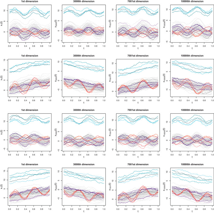
Sample datasets of the four models and selected dimensions ($p=10\hspace{0.17em}000$, $c=1$). Each model is represented in a row, with row i corresponding to the ith model. Outliers are represented according to the following color code: Magnitude, shape, and joint outliers are displayed in blue, red, and purple shades, respectively. Two non‐outlying curves are presented in black with solid and dashed lines to help visualize how the relative ordering between curves changes across dimensions, which can also be observed by monitoring the changes in position of magnitude and shape outliers marginals. In Models 1 and 3, the ordering is preserved across dimensions while in Models 2 and 4 the ordering is reversed in odd and even dimensions. In Models 1 and 2, the relative ordering of joint outliers across dimensions is random, while in Models 3 and 4, it follows a pattern opposite to that of the rest of the sample

FIGURE 6.

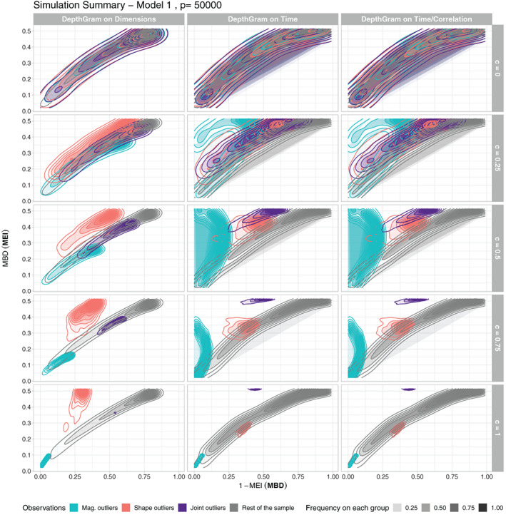
Summary of 200 simulation runs under Model 1, with $p=50\hspace{0.17em}000$, and different outlyingness values c. Summary Depthgrams are obtained as the density contours of mbd(epi) and 1‐epi(mbd) points over the 200 simulated datasets. The colors represent outlier classification (including non‐outlying observations)

These summary graphical representations indicate that as the outlyingness intensity c decreases, all the observations (outliers of different types and the rest of the sample) are mixed together, which is expected, as c represents the proportion of dimensions in which candidate outlying curves are actually simulated to present an outlying behavior. However, even for $c=0.25$, we can already find some separation between different classes of observations. Notice that in Models 2 and 4, magnitude outliers also behave as joint outliers (because they persistently exhibit average high values in every dimension, instead of alternating between high and low values); hence, it is not surprising to find them close together in the Time Depthgrams. In addition, notice how joint outliers are better distinguished when comparing Model 3 to Model 1 and Model 4 to Model 2 (especially true for lower values of c). In general, magnitude outliers are the most difficult to identify (except when they also behave as joint outliers), because even if they are always found at the left bottom corner of the Dimensions Depthgram, no separation may exist at all between them and the rest of the typical observations. In fact, this is true in this setting, for which the order of the curves is optimally preserved among dimensions. In other situations, non‐outlying observations would have average ranks over dimensions significantly smaller than magnitude outliers, and the separation would be more evident. However, the detection of magnitude and shape outliers is more of a marginal problem. In addition to the DepthGram analysis, marginal outlier detection for univariate functional data has been conducted on each dataset using conventional methods. Details on this procedure and the results obtained are provided under Supplementary Materials (Table 1).

3.2. Low‐dimensional setting

To set a reference with respect to existing methods, we compare the Depthgram with the functional outlier map (FOM), ^{15 , 17} and the magnitude‐shape plot (MS‐plot) ¹⁸ as a tool for outlier detection.

The FOM is a 2D graphical representation that can be used with any functional (integrated) depth or outlyingness measure. It displays the functional depth of each observation (obtained as aggregation of multivariate depths over the observation domain) vs a measure of variability of the multivariate depth values for each time point. Here, we consider the FOM adopted with the functional directional outlyingness (fDO) as introduced in Reference ¹⁷, for which an outlier detection rule is defined based on the distribution of the Euclidean distances of the FOM points to the origin, after scaling.

The MS‐plot adopts an alternative definition of directional outlyingness that assigns a p‐dimensional (directional) outlyingness vector to a functional p‐variate observation. The MS‐plot maps the multivariate functional data to multivariate points by representing each observation with its mean directional outlyingness vector and a measure of its variability. When $p>2$, the graphical representation can be performed by simply representing the norm of the mean outlyingness vector vs its variability. The outlier detection rule relies on the approximate distribution of the robust Mahalanobis distances of the $(p+1)$‐dimensional points in the MS‐plot.

Both outlier detection procedures are designed for low‐dimensional settings. The multivariate outlyingness measure leading to fDO in FOM is calculated using an approximate algorithm that relies on the assumption $p<n$. The MS‐plot can be obtained for any value of p; however, the associated outlier detection rule, in particular, the approximation of the distribution of the robust Mahalanobis distance, requires $p<n$. Hence, we restrict this simulation study to $p=10$ and $p=50$, keeping all other settings from the high‐dimensional case.

The two alternative methods considered bear an important computational burden as p increases, because they rely on the computation of p‐variate outlyingness measures, over each point of the observation domain. To reduce this burden, we propose an alternative way to apply these outlier detection techniques, by considering the synthetic functional multivariate datasets as functional univariate datasets defined on a multivariate domain. In other words, for each individual i, its observed p‐variate function $x_i:ℐ\to {ℝ}^p$, $x_i(t)=(x_i^1(t),\dots ,x_i^p(t))$, can be regarded as a surface or volume $x_i:ℐ\times D\to ℝ$, $x_i(t,j)=x_i^j(t)$, where D is a continuous domain, for which in practice, the process is only observed at p discretized points. From a practical perspective it implies that univariate functions are stacked together. Handling the data in this manner, the multivariate structure that may help detecting joint outliers is missed. However, we expect to identify this type of outliers as shape outliers in the new functional univariate dataset. Notice that for the Depthgram, both approaches are equivalent and yield the same results. In fact, the depth‐related quantities involved in the construction of the Depthgram are computed over the $p\times N$ grid of all the dimensions and observation points.

To establish a direct comparison in terms of detection rates, we adopt the following empirical outlier detection rule for the Depthgrams: the set of outlying observations in depthgram $k\in \{d,t,tc\}$ is $O^k=\{i=1,\dots ,n|d_i^k>Q_3(d^k)+F·IQR(d^k)\}$, where $d_i^k=D{G}_{i2}^k-g_n(D{G}_{i1}^k)$, $i=1,\dots ,n$, and $Q_3$ and $IQR$ denote the sample third quartile and interquartile range, respectively. The global set of outlying observations is defined as $O=O^d\cup O^t\cup O^{tc}$. The factor F is set to 1.5, similar to the classical boxplot rule. For this procedure, which is inspired by Proposition 1, to yield accurate results, we would need a data‐driven estimation approach to approximate F, similar to the adjusted outliergram. ⁶ However, this will require us to approximate the distribution of $d^k$, $k\in \{d,t,tc\}$, which is unfeasible in a high‐dimensional setting, and is beyond the scope of this article. Here, the objective is to provide a simple rule to conduct the comparative analysis. Notice that the graphical summaries that have been used in the high‐dimensional simulation study to visually assess the performance of the Depthgram cannot be adopted with the other two methods because the quantities represented in the FOM and MS‐plot are the mean and dispersion of outlyingness values, which are not bounded and might even exhibit very different ranges across simulation runs.

In Figures 7 and 8, we present the five graphical tools for two different simulation runs with $p=50$ from Models 1 and 2, respectively. We can find similar graphical representations for Models 3 and 4, under Supplementary Materials. In all simulation runs, outliers are coded as observations 86 to 100: labels 86 to 90 (blue shades in the figures) correspond to magnitude outliers, 91 to 95 (pink/red shades in the figures) correspond to shape outliers, and labels 96 to 100 represent joint outliers (purple shades in the figures). Tables 2 and 3 under Supplementary Materials contain the proportion of correctly and falsely identified outliers by each one of the methods, over the 200 simulation runs for the four models and different values of p. Accordingly, we can draw the following conclusions. The Depthgram behaviors for both $p=10,50$ are very similar to the one observed in a high‐dimensional setting, with slightly better detection rates for $p=50$: shape outliers are detected by the Time Depthgram, joint outliers are detected by the Time/Correlation Depthgram and magnitude outliers are only detected when they are also joint outliers (Models 2 and 4 with negative association among components). In general, FOM exhibits a low detection rate, with better performance in the lower dimension case ($p=10$) and in its p‐dimensional version, except for magnitude outliers, which are also captured in its $one$‐dimensional version. For the MS‐plot, detection rates are generally very high, with better performance for $p=10$ in its p‐dimensional version and for $p=50$ in its $one$‐dimensional version. For this configuration ($p=50$, MS‐plot 1‐dim), the method exhibits full detection capacity in models with positive association among components (Models 1 and 3). However, for Models 2 and 4, there is a high false positive detection rate (around $10\%$) and low sensitivity for shape (both models) and joint outliers (Model 2). The Depthgram exhibits the best overall detection performance for joint outliers. Regarding the p‐dimensional versions of FOM and MS‐plot, the drop, as c reaches the value 1, of the proportion of correctly detected magnitude (both) and shape outliers (only for FOM) is worth noting. This might be owing to the fact that for $c=1$, all 15 potential outliers consistently act as outliers in every dimension, which increases the contamination level on the p‐dimensional spaces associated to each time point (where multivariate outlyingness measures are applied).

FIGURE 7.

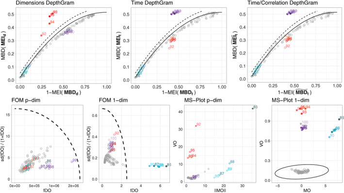
Results for a single simulation run under Model 1, with $p=50$, and $c=1$. In the top row we present the three DepthGram representations. In the bottom row, we present the FOM and the MS‐plot in their p‐dimensional and 1‐dimensional versions. Except for the p‐dimensional MS‐plot, the boundary dividing the outlying and non‐outlying observations is drawn (a dashed line for the DepthGram and FOM and a solid ellipse for the MS‐plot). In all the plots, detected outliers are marked with a bullet while the rest of the observations are represented with an empty circle. True outliers are represented in color (blue for magnitude outliers, pink/red for shape outliers and purple for joint outliers) while non‐outlying observations are drawn in gray

FIGURE 8.

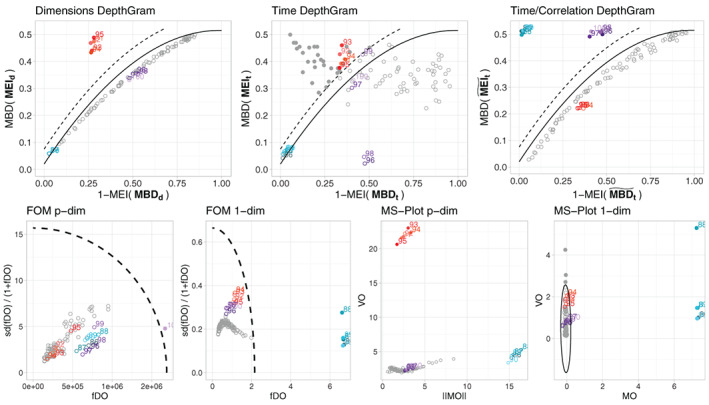
Results for a single simulation run under Model 2, with $p=50$, and $c=1$. In the top row we present the three DepthGram representations. In the bottom row, we present the FOM and the MS‐plot in their p‐dimensional and 1‐dimensional versions. Except for the p‐dimensional MS‐plot, the boundary dividing the outlying and non‐outlying observations is drawn (a dashed line for the DepthGram and FOM and a solid ellipse for the MS‐plot). In all the plots, detected outliers are marked with a bullet while the rest of the observations are represented with a circle. True outliers are represented in color (blue for magnitude outliers, pink/red for shape outliers and purple for joint outliers) while non‐outlying observations are drawn in gray

As we have mentioned in the previous section, marginal (shape and magnitude) outliers can be detected very efficiently with univariate functional detection methods. Moreover, these have the advantage, over multivariate methods, of identifying the components in which the outlying behavior happens. Thus, multivariate methods should focus on the detection of joint outliers, which, as we have seen, might be difficult in the presence of different types of outlying observations and, especially, negative association among dimensions. This can be explained by the fact that for methods based on the functional one‐dimensional representation, negative association becomes shape variability among the curves, and the higher the variability in the sample, the more difficult it is to detect outlying curves. However, for the original versions of FOM and MS‐plot, the underlying multivariate outlyingness measures are significantly influenced by the presence of other types of outliers.

Another point for comparison is the computational complexity of the different methods. DepthGram is a very efficient procedure because it is based on the computations of MBD and MEI, which solely requires the ranking of observations at any time point and dimension. The outlyingness measures adopted for the FOM and MS‐plot representations are heavier from a computational perspective, and even in their one‐dimensional configuration, in which they are computed over samples of real numbers at every time point and dimension, the computation times are significantly higher than those of DepthGram (refer to Supplementary Materials for details).

4. tFMRI DATA EXPLORATION

In this section, we analyze two tfMRI experiments conducted on the same $n=100$ healthy individuals (the analysis of two other tasks on the same individuals is included under Supplementary Materials). Data (T1‐weighted, T1w, and two tfMRI) were obtained from the HCP database (https://db.humanconnectome.org/), which are comprehensively described in Reference ²³. Only the tfMRI acquired during two different functional tasks were selected for this study. The first stack of tfMRIs were acquired during a motor task where some visual cues requested the participants to either tap their left or right fingers. The second acquisition was performed during a language task where different stories or arithmetic operations were presented to the participants via an audio record, and after having listened to them, they were asked a question about what they heard, and two possible answers were offered to be selected by pushing a button. Task and resting periods were alternated during a total duration of $T=284$ and 316 seconds for the motor and language experiments, respectively.

Together with the native T1w and tfMRI images, HCP provided the minimal preprocessed images, ²⁴ which includes the tfMRI images spatially registered to a stereotactic space (MNI, Montreal Neurological Institute). These normalized images ($FOV=91\times 109\times 91$ voxels of 2 mm isotropic resolution) were the images used in this study. A binary image (1 = brain, 0 = background) defined in the MNI space was employed to select 192 631 voxels.

The final datasets are thus composed by the brain activity records of $n=100$ subjects on $p=192\hspace{0.17em}631$ points of the brain over $T=284$ and $T=316$ seconds. The objective of the analysis is to help visualize this high‐dimensional functional dataset and to detect individuals with central and outlying brain activity patterns. As an example, Figure 9 presents the brain signals over time in 6 selected voxels for the motor experiment. Four individuals are highlighted to help visualize alterations in signal shape and in association patterns across dimensions (voxels).

FIGURE 9.

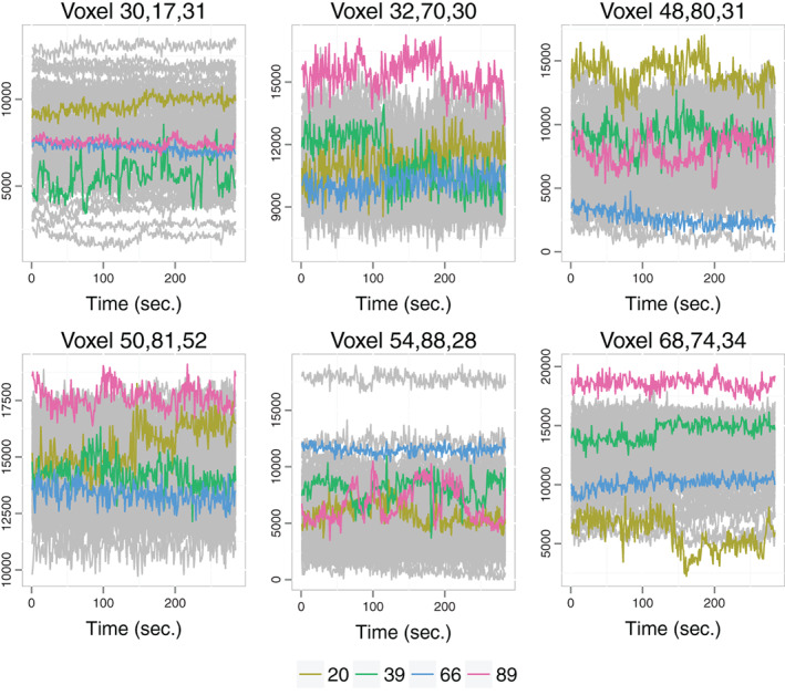
Brain activity over time of $n=100$ individuals in 6 of the $p=192\hspace{0.17em}631$ voxels for the motor experiment. The signals of individuals 20, 39, 66, and 89 are highlighted. These are some of the individuals identified as potential outliers, except for individual 66 who exhibits the most central pattern (Figure 10). They illustrate different signal shapes and different association patterns across voxels. For instance, individual 20 presents negative association between voxels 48, 80, 31 (top right) and 68, 74, 34 (bottom right) while this association is positive for the other three individuals

Depthgrams for the motor experiment are illustrated in Figure 10. The time Depthgram is significantly spread on both dimensions, which implies that mixing/crossing of individual signals exist across dimensions (voxels). When considering the time/correlation Depthgram, point coordinates differ; however, the global structure remains the same. This heterogeneity across voxels does not follow a structured pattern, and is rather the result of independent components. This might be owing to the fact that only very specific regions of the brain are involved, and are expected to be activated in the motor task. Hence, the signals of the voxels outside of these regions act as noise in this experiment, thereby inducing this independence pattern across voxels.

FIGURE 10.

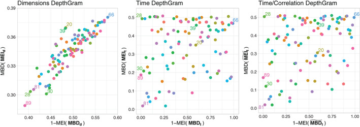
DepthGrams for the motor experiment

In Figure 11, we present the same views, but this time for the language experiment. Here, we can observe how the time and time/correlation Depthgrams follow the same unstructured pattern as in the motor experiment, because, again, the regions involved in the language task represent a small part of the entire brain.

FIGURE 11.

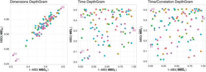
DepthGrams for the language experiment

Regarding outlier detection, let us first point out that the analyzed dataset meets quality standards in the field because clinical diagnosis for several mental conditions were considered to exclude subjects from the experiment, and standard fMRI techniques for artifact removal had been applied as a preprocessing step. Moreover, due to the general independence of signals across voxels, we cannot expect to find any joint outlier, as explained in Section 2.3. Indeed, if there is no common association pattern across voxels shared by a majority of individuals, deviances from it cannot be observed (refer to the Supplementary Materials for different results on two additional task datasets). Nevertheless, the Depthgrams have enabled the identification of some outlying patients. In the motor experiment, individual 39 is located in the north‐west area of the voxel Depthgram as a potential shape outlier. After the posterior examination, this subject happens to have moved more than permissible during the experiment, and thus should have been discarded from the sample. The same is observed with subject 84 in the language experiment, that would be classified as a magnitude outlier. This different consideration of the outlier type in these two cases, which tend to share the same source of noise, might be owing to the different nature of the task performed in each experiment and the interference of motion. Moreover, individual 81, which appears to be a magnitude outlier in the language experiment, has been demonstrated, by a posterior examination, to suffer a mild form of schizophrenia that had not been diagnosed. Additionally, marginal outlier detection has been applied voxel‐wise. The results for both experiments indicate that all individuals exhibit a magnitude and/or shape outlying behavior in at least some hundreds of dimensions, out of a total of 192 631 voxels. However, if we just consider individuals with an outlying behavior in a large number of voxels, the results are consistent with those potential shape and magnitude outliers identified with the Depthgrams.

5. DISCUSSION

This study proposed the Depthgram as a tool for representing high‐dimensional functional observations on a plane. Unlike current approaches for multivariate functional depth based on aggregation over dimensions or time of suitable functional or multivariate depth measures, the proposed methodology relies on the depth of depths. In fact, the variables that define the two‐dimensional representation of the data are depth measures/indexes on the datasets obtained by computing depth over dimensions or time domain. This approach enables the identification of different types of outliers in different parts of the plot, including joint outliers. It is computationally efficient in the high‐dimensional setting, and unlike procedures relying on outlyingness measures, it also facilitates a global overview of the sample composition. The methodology relies on the theoretical relationship between two different depth of depths measures. The result allows establishing the most likely regions for typical and atypical observations. However, it does not provide an outlying detection rule because the distribution of the distance to the theoretical boundary for typical and atypical observations is unknown and cannot be feasibly approximated in the high‐dimensional setting. Nevertheless, an empirical detection rule can be adopted by setting a cutoff value for point distances to the boundary.

There are three versions of the Depthgram: dimensions, time and time/correlation depthgrams. They are designed to be used together because they provide complementary information. The first version is the most useful at identifying shape and magnitude outliers. The time Depthgram aims at identifying joint outliers, that is, observations that are not marginal outliers in any of the dimensions, but exhibit a dependency pattern among dimensions that differs from the rest of the sample. The time/correlation Depthgram is designed to do the same in situations where the general association pattern among dimensions is highly variable and the time Depthgram fails to provide a structured representation of the sample. In fact, the comparison of the time and time/correlation depthgrams elucidates the association patterns across dimensions, where the association in this case is understood as linear correlation among the curve ranks given by the modified epigraph index. In general, for the three Depthgrams, the more similar and smooth the curves, and the more regular the association pattern in the sample, the more structured the Depthgram representations. In other words, we can also better understand the regularity or homogeneity of the sample by the spread of the Depthgrams representations.

Finally, we suggest the combination of the Depthgram with specific tools for the detection of marginal outliers across the different univariate functional samples. Certainly, the challenge with a high‐dimensional functional setting, and which cannot be achieved with existing tools for univariate functional data is the ability to detect atypical joint behavior. If marginal outliers are present in the sample, not only is it more efficient to adopt specific methods marginally, but it is also more beneficial to identify the dimensions in which the observation exhibits an outlying behavior than just classifying the entire observation as an outlier. Accordingly, we recommend the use of the functional boxplot ⁵ and the outliergram, ⁶ as they rely on the same depth tools than the Depthgram and can be computed simultaneously and efficiently.

Supporting information

Data S1 Supplementary material

Alemán‐Gómez Y, Arribas‐Gil A, Desco M, Elías A, Romo J. Depthgram: Visualizing outliers in high‐dimensional functional data with application to fMRI data exploration. Statistics in Medicine. 2022;41(11):2005–2024. doi: 10.1002/sim.9342

DATA AVAILABILITY STATEMENT

The data that support the findings of this study are openly available in the HCP database (https://db.humanconnectome.org/), listed under HCP 1200 Subject Release‐100 unrelated subjects, datasets: Language Task fMRI Preprocessed, Motor Task fMRI Preprocessed, Emotion Task fMRI Preprocessed, Gambling Task fMRI Preprocessed. They are described in detail in Reference ²³.

REFERENCES

- 1. Littlejohns T, Holliday J, Gibson L, et al. The UK Biobank imaging enhancement of 100,000 participants: rationale, data collection, management and future directions. Nat Commun. 2020;11:2624. doi: 10.1038/s41467-020-15948-9 [DOI] [PMC free article] [PubMed] [Google Scholar]
- 2. Feldstein‐Ewing SW, Luciana M, eds. The Adolescent Brain Cognitive Development (ABCD) consortium: rationale, aims, and assessment strategy (special issue). Dev Cogn Neurosci. 2018;32:1‐164.29496476 [Google Scholar]
- 3. Barch DM, Burgess GC, Harms MP, et al. Function in the human connectome: task‐fMRI and individual differences in behavior. NeuroImage. 2013;80:169‐189. [DOI] [PMC free article] [PubMed] [Google Scholar]
- 4. Zhang S, Li X, Lv J, Jiang X, Guo L, Liu T. Characterizing and differentiating task‐based and resting state fMRI signals via two‐stage sparse representations. Brain Imaging Behav. 2016;10:21‐32. [DOI] [PMC free article] [PubMed] [Google Scholar]
- 5. Sun Y, Genton MG. Functional boxplots. J Comput Graph Stat. 2011;20:316‐334. [Google Scholar]
- 6. Arribas‐Gil A, Romo J. Shape outlier detection and visualization for functional data: the outliergram. Biostatistics. 2014;15(4):603‐619. [DOI] [PubMed] [Google Scholar]
- 7. Chiou JM, Müller HG. Linear manifold modelling of multivariate functional data. J R Stat Soc Ser B. 2014;76:605‐626. [Google Scholar]
- 8. Ieva F, Paganoni AM. Depth measures for multivariate functional data. Commun Stat Theory Methods. 2013;42(7):1265‐1276. [Google Scholar]
- 9. Zipunnikov V, Caffo B, Yousem DM, Davatzikos C, Schwartz BS, Crainiceanu C. Multilevel functional principal component analysis for high‐dimensional data. J Comput Graph Stat. 2011;20(4):852‐873. doi: 10.1198/jcgs.2011.10122 [DOI] [PMC free article] [PubMed] [Google Scholar]
- 10. Happ C, Greven S. Multivariate functional principal component analysis for data observed on different (dimensional) domains. J Am Stat Assoc. 2018;113(522):649‐659. doi: 10.1080/01621459.2016.1273115 [DOI] [Google Scholar]
- 11. Vinue G, Epifanio I. Robust archetypoids for anomaly detection in big functional data. ADAC. 2021;15:437‐462. doi: 10.1007/s11634-020-00412-9 [DOI] [Google Scholar]
- 12. López‐Pintado S, Romo J. On the concept of depth for functional data. J Am Stat Assoc. 2009;104(486):718‐734. [Google Scholar]
- 13. Claeskens G, Hubert MLS, Vakili K. Multivariate functional halfspace depth. J Am Stat Assoc. 2014;109(505):411‐423. [Google Scholar]
- 14. Ieva F, Paganoni AM. Component‐wise outlier detection methods for robustifying multivariate functional samples. Stat Pap. 2020;61(2):595‐614. doi: 10.1007/s00362-017-0953-1 [DOI] [Google Scholar]
- 15. Hubert M, Rousseeuw P, Segaert P. Multivariate functional outlier detection. JISS. 2015;24:177‐202. [Google Scholar]
- 16. Nieto‐Reyes A, Cuesta‐Albertos JA. Hubert, Rousseeuw and Segaert: multivariate functional outlier detection. JISS. 2015;24:237‐243. [Google Scholar]
- 17. Rousseeuw PJ, Raymaekers J, Hubert M. A measure of directional outlyingness with applications to image data and video. J Comput Graph Stat. 2018;27(2):345‐359. [Google Scholar]
- 18. Dai W, Genton MG. Multivariate functional data visualization and outlier detection. J Comput Graph Stat. 2018;27(4):923‐934. doi: 10.1080/10618600.2018.1473781 [DOI] [Google Scholar]
- 19. Arribas‐Gil A, Romo J. Discussion of "Multivariate functional outlier detection". JISS. 2015;24:263‐267. [Google Scholar]
- 20. Cuesta‐Albertos J, Nieto‐Reyes A. The random Tukey depth. Comput Stat Data Anal. 2008;52(11):4979‐4988. doi: 10.1016/j.csda.2008.04.021 [DOI] [Google Scholar]
- 21. Sun Y, Genton MG, Nychka DC. Exact fast computation of band depth for large functional datasets: How quickly can one million curves be ranked? Stat. 2012;1:68‐74. [Google Scholar]
- 22. López‐Pintado S, Romo J. A half‐region depth for functional data. Comput Stat Data Anal. 2011;55:1679‐1695. [Google Scholar]
- 23. Hodge MR, Horton W, Brown T, et al. ConnectomeDB ‐ sharing human brain connectivity data. NeuroImage. 2016;124 B:1102‐1107. [DOI] [PMC free article] [PubMed] [Google Scholar]
- 24. Glasser MF, Smith SM, Marcus DS, et al. The human connectome project's neuroimaging approach. Nat Neurosci. 2016;19:1175‐1187. [DOI] [PMC free article] [PubMed] [Google Scholar]
- 25. Ieva F, Paganoni AM, Romo J, Tarabelloni N. roahd package: robust analysis of high dimensional data. R J. 2019;11(2):291‐307. doi: 10.32614/RJ-2019-032 [DOI] [Google Scholar]
Associated Data
This section collects any data citations, data availability statements, or supplementary materials included in this article.
Supplementary Materials