LDLE: Low Distortion Local Eigenmaps

Abstract

We present Low Distortion Local Eigenmaps (LDLE), a manifold learning technique which constructs a set of low distortion local views of a data set in lower dimension and registers them to obtain a global embedding. The local views are constructed using the global eigenvectors of the graph Laplacian and are registered using Procrustes analysis. The choice of these eigenvectors may vary across the regions. In contrast to existing techniques, LDLE can embed closed and non-orientable manifolds into their intrinsic dimension by tearing them apart. It also provides gluing instruction on the boundary of the torn embedding to help identify the topology of the original manifold. Our experimental results will show that LDLE largely preserved distances up to a constant scale while other techniques produced higher distortion. We also demonstrate that LDLE produces high quality embeddings even when the data is noisy or sparse.

1. Introduction

Manifold learning techniques such as Local Linear Embedding (Roweis and Saul, 2000), Diffusion maps (Coifman and Lafon, 2006), Laplacian eigenmaps (Belkin and Niyogi, 2003), t-SNE (Maaten and Hinton, 2008) and UMAP (McInnes et al., 2018), aim at preserving local information as they map a manifold embedded in higher dimension into lower (possibly intrinsic) dimension. In particular, UMAP and t-SNE follow a top-down approach as they start with an initial low-dimensional global embedding and then refine it by minimizing a local distortion measure on it. In contrast, similar to LTSA (Zhang and Zha, 2003) and (Singer and Wu, 2011), a bottom-up approach for manifold learning can be conceptualized to consist of two steps, first obtaining low distortion local views of the manifold in lower dimension and then registering them to obtain a global embedding of the manifold. In this paper, we take this bottom-up perspective to embed a manifold in low dimension, where the local views are obtained by constructing coordinate charts for the manifold which incur low distortion.

1.1. Local Distortion

Let $\left(\mathcal{M},g\right)$ be a d-dimensional Riemannian manifold with finite volume. By definition, for every x_k in $\mathcal{M}$, there exists a coordinate chart $\left({\mathcal{U}}_k,{\mathrm{\Phi }}_k\right)$ such that $x_k\in {\mathcal{U}}_k$, ${\mathcal{U}}_k\subset M$ and Φ_k maps ${\mathcal{U}}_k$ into ${ℝ}^d$. One can envision ${\mathcal{U}}_k$ to be a local view of $\mathcal{M}$ in the ambient space. Using rigid transformations, these local views can be registered to recover $\mathcal{M}$. Similarly, ${\mathrm{\Phi }}_k\left({\mathcal{U}}_k\right)$ can be viewed to be a local view of $\mathcal{M}$ in the d-dimensional embedding space ${ℝ}^d$. Again, using rigid transformations, these local views can be registered to obtain the d-dimensional embedding of $\mathcal{M}$.

As there may exist multiple mappings which map ${\mathcal{U}}_k$ into ${ℝ}^d$, a natural strategy would be to choose a mapping with low distortion. Multiple measures of distortion exist in literature (Vankadara and Luxburg, 2018). The measure of distortion used in this work is as follows. Let d_g(x,y) denote the shortest geodesic distance between $x,y\in \mathcal{M}$. The distortion of Φ_k on ${\mathcal{U}}_k$ as defined in (Jones et al., 2007) is given by

$$\text{Distortion}\left({\mathrm{\Phi }}_k,{\mathcal{U}}_k\right)={‖{\mathrm{\Phi }}_k‖}_{\text{Lip}}{‖{\mathrm{\Phi }}_k^{-1}‖}_{\text{Lip}}$$ (1)

where ${‖{\mathrm{\Phi }}_k‖}_{\text{Lip}}$ is the Lipschitz norm of Φ_k given by

$${‖{\mathrm{\Phi }}_k‖}_{\text{Lip}}=\underset{\begin{array}{c}x,y\in {\mathcal{U}}_k\\ x\ne y\end{array}}{\sup }\frac{{‖{\mathrm{\Phi }}_k\left(x\right)-{\mathrm{\Phi }}_k\left(y\right)‖}_2}{d_g\left(x,y\right)},$$ (2)

and similarly,

$${‖{\mathrm{\Phi }}_k^{-1}‖}_{\text{Lip}}=\underset{\begin{array}{c}x,y\in {\mathcal{U}}_k\\ x\ne y\end{array}}{\sup }\frac{d_g\left(x,y\right)}{{‖{\mathrm{\Phi }}_k\left(x\right)-{\mathrm{\Phi }}_k\left(y\right)‖}_2}.$$ (3)

Note that Distortion $\left({\mathrm{\Phi }}_k,{\mathcal{U}}_k\right)$ is always greater than or equal to 1. If Distortion $\left({\mathrm{\Phi }}_k,{\mathcal{U}}_k\right)=1$, then Φ_k is said to have no distortion on ${\mathcal{U}}_k$. This is achieved when the mapping Φ_k preserves distances between points in ${\mathcal{U}}_k$ up to a constant scale, that is, when Φ_k is a similarity on ${\mathcal{U}}_k$. It is not always possible to obtain a mapping with no distortion. For example, there does not exist a similarity which maps a locally curved region on a surface into a Euclidean plane. This follows from the fact that the sign of the Gaussian curvature is preserved under simil arity transformation which in turn follows from the Gauss’s Theorema Egregium.

1.2. Our Contributions

This paper takes motivation from the work in (Jones et al., 2007) where the authors provide guarantees on the distortion of the coordinate charts of the manifold constructed using carefully chosen eigenfunctions of the Laplacian. However, this only applies to the charts for small neighborhoods on the manifold and does not provide a global embedding. In this paper, we present an approach to realize their work in the discrete setting and obtain low-dimensional low distortion local views of the given data set using the eigenvectors of the graph Laplacian. Moreover, we piece together these local views to obtain a global embedding of the manifold. The main contributions of our work are as follows:

1. We present an algorithmic realization of the construction procedure in (Jones et al., 2007) that applies to the discrete setting and yields low-dimensional low distortion views of small metric balls on the given discretized manifold (See Section 2 for a summary of their procedure).

2. We present an algorithm to obtain a global embedding of the manifold by registering its local views. The algorithm is designed so as to embed closed as well as non-orientable manifolds into their intrinsic dimension by tearing them apart. It also provides gluing instructions for the boundary of the embedding by coloring it such that the points on the boundary which are adjacent on the manifold have the same color (see Figure 2).

Figure 2:

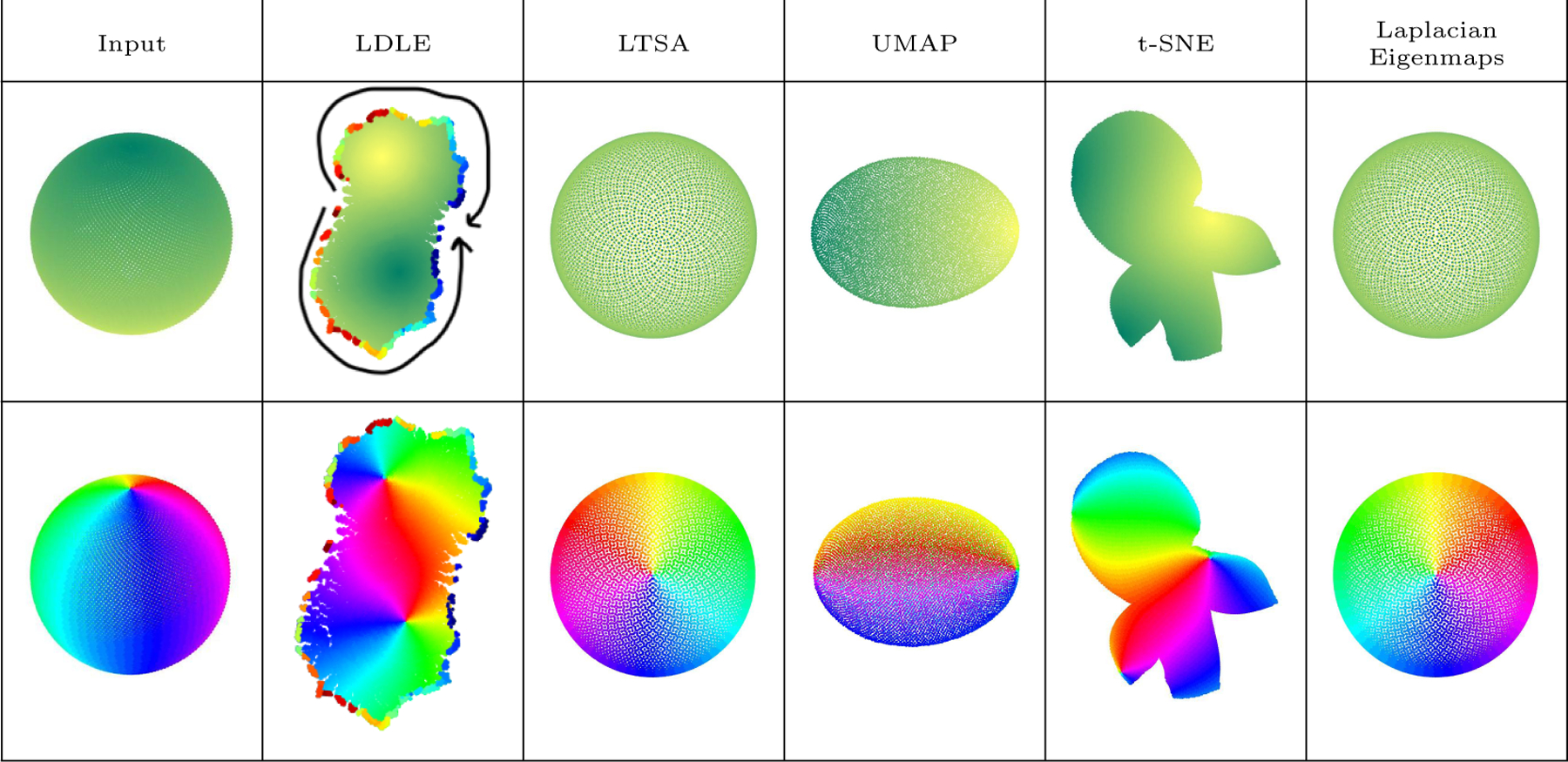
Embeddings of a sphere in ${ℝ}^3$ into ${ℝ}^2$. The top and bottom row contain the same plots colored by the height and the azimuthal angle of the sphere (0 − 2π), respectively. LDLE automatically colors the boundary so that the points on the boundary which are adjacent on the sphere have the same color. The arrows are manually drawn to help the reader identify the two pieces of the boundary which are to be stitched together to recover the original sphere. LTSA, UMAP and Laplacian eigenmaps squeezed the sphere into different viewpoints of ${ℝ}^2$ (side or top view of the sphere). t-SNE also tore apart the sphere but the embedding lacks interpretability as it is “unaware” of the boundary.

LDLE consists of three main steps. In the first step, we estimate the inner product of the Laplacian eigenfunctions’ gradients using the local correlation between them. These estimates are used to choose eigenfunctions which are in turn used to construct low-dimensional low distortion parameterizations Φ_k of the small balls U_k on the manifold. The choice of the eigenfunctions depend on the underlying ball. A natural next step is to align these local views Φ_k(U_k) in the embedding space, to obtain a global embedding. One way to align them is to use Generalized Procrustes Analysis (GPA) (Crosilla and Beinat, 2002; Gower, 1975; Ten Berge, 1977). However, we empirically observed that GPA is less efficient and prone to errors due to large number of local views with small overlaps between them. Therefore, motivated from our experimental observations and computational necessity, in the second step, we develop a clustering algorithm to obtain a small number of intermediate views ${\tilde{\mathrm{\Phi }}}_m\left({\tilde{U}}_m\right)$ with low distortion, from the large number of smaller local views Φ_k(U_k). This makes the subsequent GPA based registration procedure faster and less prone to errors.

Finally, in the third step, we register intermediate views ${\tilde{\mathrm{\Phi }}}_m\left({\tilde{U}}_m\right)$ using an adaptation of GPA which enables tearing of closed and non-orientable manifolds so as to embed them into their intrinsic dimension. The results on a 2D rectangular strip and a 3D sphere are presented in Figures 1 and 2, to motivate our approach.

Figure 1:

Embeddings of a rectangle (4 × 0.25) with high aspect ratio in ${ℝ}^2$ into ${ℝ}^2$.

The paper organization is as follows. Section 2 provides relevant background and motivation. In Section 3 we present the construction of low-dimensional low distortion local parameterizations. Section 4 presents our clustering algorithm to obtain intermediate views. Section 5 registers the intermediate views to a global embedding. In Section 6 we compare the embeddings produced by our algorithm with existing techniques on multiple data sets. Section 7 concludes our work and discusses future directions.

1.3. Related Work

Laplacian eigenfunctions are ubiquitous in manifold learning. A large proportion of the existing manifold learning techniques rely on a fixed set of Laplacian eigenfunctions, specifically, on the first few non-trivial low frequency eigenfunctions, to construct a low-dimensional embedding of a manifold in high dimensional ambient space. These low frequency eigenfunctions not only carry information about the global structure of the manifold but they also exhibit robustness to the noise in the data (Coifman and Lafon, 2006). Laplacian eigenmaps (Belkin and Niyogi, 2003), Diffusion maps (Coifman and Lafon, 2006) and UMAP (McInnes et al., 2018) are examples of such top-down manifold learning techniques. While there are limited bottom-up manifold learning techniques in the literature, to the best of our knowledge, none of them makes use of Laplacian eigenfunctions to construct local views of the manifold in lower dimension.

LTSA is an example of a bottom-up approach for manifold learning whose local mappings project local neighborhoods onto the respective tangent spaces. A local mapping in LTSA is a linear transformation whose columns are the principal directions obtained by applying PCA on the underlying neighborhood. These directions form an estimate of the basis for the tangent space. Having constructed low-dimensional local views for each neighborhood, LTSA then aligns all the local views to obtain a global embedding. As discussed in their work and as we will show in our experimental results, LTSA lacks robustness to the noise in the data. This further motivates our approach of using robust low-frequency Laplacian eigenfunctions for the construction of local views. Moreover, due to the specific constraints used in their alignment, LTSA embeddings fail to capture the aspect ratio of the underlying manifold (see Appendix F for details).

Laplacian eigenmaps uses the eigenvectors corresponding to the d smallest eigenvalues (excluding zero) of the normalized graph Laplacian to embed the manifold in ${ℝ}^d$. It can also be perceived as a top-down approach which directly obtains a global embedding that minimizes Dirichlet energy under some constraints. For manifolds with high aspect ratio, in the context of Section 1.1, the distortion of the local parameterizations based on the restriction of these eigenvectors on local neighborhoods, could become extremely high. For example, as shown in Figure 1, the Laplacian eigenmaps embedding of a rectangle with an aspect ratio of 16 looks like a parabola. This issue is explained in detail in (Saito, 2018; Chen and Meila, 2019; Dsilva et al., 2018; Blau and Michaeli, 2017).

UMAP, to a large extent, resolves this issue by first computing an embedding based on the d non-trivial low-frequency eigenvectors of a symmetric normalized Laplacian and then “sprinkling” white noise in it. It then refines the noisy embedding by minimizing a local distortion measure based on fuzzy set cross entropy. Although UMAP embeddings seem to be topologically correct, they occasionally tend to have twists and sharp turns which may be unwanted (see Figure 1).

t-SNE takes a different approach of randomly initializing the global embedding, defining a local t-distribution in the embedding space and local Gaussian distribution in the high dimensional ambient space, and finally refining the embedding by minimizing the Kullback–Leibler divergence between the two sets of distributions. As shown in Figure 1, t-SNE tends to output a dissected embedding even when the manifold is connected. Note that the recent work by Kobak and Linderman (2021) showed that t-SNE with spectral initialization results in a similar embedding as that of UMAP. Therefore, in this work, we display the output of the classic t-SNE construction, with random initialization only.

A missing feature in existing manifold learning techniques is their ability to embed closed manifolds into their intrinsic dimensions. For example, a sphere in ${ℝ}^3$ is a 2-dimensional manifold which can be represented by a connected domain in ${ℝ}^2$ with boundary gluing instructions provided in the form of colors. We solve this issue in this paper (see Figure 2).

2. Background and Motivation

Due to their global nature and robustness to noise, in our bottom-up approach for manifold learning, we propose to construct low distortion (see Eq. (1)) local mappings using low frequency Laplacian eigenfunctions. A natural way to achieve this is to restrict the eigenfunctions on local neighborhoods. Unfortunately, the common trend of using first d non-trivial low frequency eigenfunctions to construct these local mappings fails to produce low distortion on all neighborhoods. This directly follows from the Laplacian Eigenmaps embedding of a high aspect-ratio rectangle shown in Figure 1. The following example explains that even in case of unit aspect-ratio, a local mapping based on the same set of eigenfunctions would not incur low distortion on each neighborhood, while mappings based on different sets of eigenfunctions may achieve that.

Consider a unit square [0,1]×[0,1] such that for every point x_k in the square, ${\mathcal{U}}_k$ is the disc of radius 0.01 centered at x_k. Consider a mapping ${\mathrm{\Phi }}_1^{\ast }$ based on the first two non-trivial eigenfunctions cos(πx) and cos(πy) of the Laplace-Beltrami operator on the square with Neumann boundary conditions, that is,

$${\mathrm{\Phi }}_1^{\ast }\left(x,y\right)=\left(\cos \left(\pi x\right),\cos \left(\pi y\right)\right).$$ (4)

As shown in Figure 3, ${\mathrm{\Phi }}_1^{\ast }$ maps the discs along the diagonals to other discs. The discs along the horizontal and vertical lines through the center are mapped to ellipses. The skewness of these ellipses increases as we move closer to the middle of the edges of the unit square. Thus, the distortion of ${\mathrm{\Phi }}_1^{\ast }$ is low on the discs along the diagonals and high on the discs close to the middle of the edges of the square.

Figure 3:

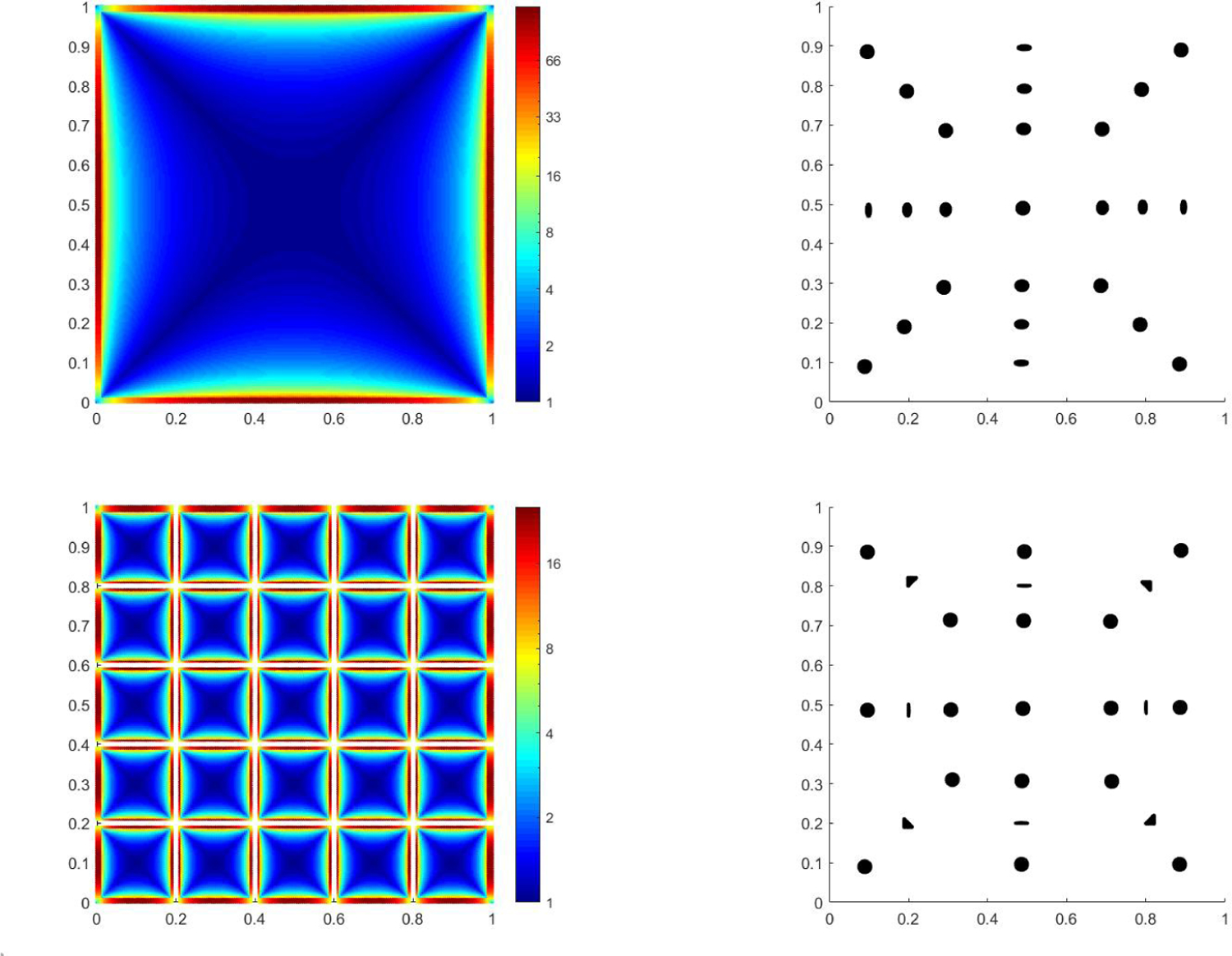
(Left) Distortion of ${\mathrm{\Phi }}_1^{\ast }$ (top) and ${\mathrm{\Phi }}_2^{\ast }$ (bottom) on discs of radius 0.01 centered at (x,y) for all x, y ∈ [0, 1] × [0, 1]. ${\mathrm{\Phi }}_2^{\ast }$ produces close to infinite distortion on the discs located in the white region. (Right) Mapping of the discs at various locations in the square using ${\mathrm{\Phi }}_1^{\ast }$ (top) and ${\mathrm{\Phi }}_2^{\ast }$ (bottom).

Now, consider a different mapping based on another set of eigenfunctions,

$${\mathrm{\Phi }}_2^{\ast }\left(x,y\right)=\left(\cos \left(5\pi x\right),\cos \left(5\pi y\right)\right).$$ (5)

Compared to ${\mathrm{\Phi }}_1^{\ast }$, ${\mathrm{\Phi }}_2^{\ast }$ produces almost no distortion on the discs of radius 0.01 centered at (0.1, 0.5) and (0.9, 0.5) (see Figure 3). Therefore, in order to achieve low distortion, it seem to make sense to construct local mappings for different regions based on different sets of eigenfunctions.

The following result from (Jones et al., 2007) manifests the above claim as it shows that, for a given small neighborhood on a Riemannian manifold, there always exist a subset of Laplacian eigenfunctions such that a local parameterization based on this subset is bilipschitz and has bounded distortion. A more precise statement follows.

Theorem 1 ((Jones et al., 2007), Theorem 2.2.1). Let $\left(\mathcal{M},g\right)$ be a d-dimensional Riemannian manifold. Let ∆_g be the Laplace-Beltrami operator on it with Dirichlet or Neumann boundary conditions and let ϕ_i be an eigenfunction of ∆_g with eigenvalue λ_i. Assume that $\left|\mathcal{M}\right|=1$ where $\left|\mathcal{M}\right|$ is the volume of $\mathcal{M}$ and the uniform ellipticity conditions for ∆_g are satisfied. Let $x_k\in \mathcal{M}$ and r_k be less than the injectivity radius at x_k (the maximum radius where the the exponential map is a diffeomorphism). Then, there exists a constant κ > 1 which depends on d and the metric tensor g such that the following hold. Let ρ ≤ r_k and $B_k\equiv B_{{\kappa }^{-1}\rho }\left(x_k\right)$ where

$$B_{ϵ}\left(x\right)=\left\{y\in \mathcal{M}|d_g\left(x,y\right)<ϵ\right\}.$$ (6)

Then there exist i₁,i₂,...,i_d such that, if we let

$${\gamma }_{ki}={\left(\frac{{\displaystyle {\int }_{B_k}{\varphi }_i^2\left(y\right)dy}}{\left|B_k\right|}\right)}^{-1/2}$$ (7)

then the map

$$\begin{array}{l}{\mathrm{\Phi }}_k:B_k\to {ℝ}^d\\ \hspace{1em} \hspace{1em}\hspace{0.17em}x\to \left({\gamma }_{k{i}_1}{\varphi }_{i_1}\left(x\right),\dots ,{\gamma }_{k{i}_d}{\varphi }_{i_d}\left(x\right)\right)\end{array}$$ (8)

is bilipschitz such that for any y₁,y₂ ∈ B_k it satisfies

$$\frac{{\kappa }^{-1}}{\rho }{d}_g\left(y_1,y_2\right)\le ‖{\mathrm{\Phi }}_k\left(y_1\right)-{\mathrm{\Phi }}_k\left(y_2\right)‖\le \frac{\kappa }{\rho }{d}_g\left(y_1,y_2\right),$$ (9)

where the associated eigenvalues satisfy

$${\kappa }^{-1}{\rho }^{-2}\le {\lambda }_{i_1},\dots ,{\lambda }_{i_d}\le \kappa {\rho }^{-2},$$ (10)

and the distortion is bounded from above by κ² i.e.

$$\underset{\begin{array}{c}{y}_1,y_2\in B_k\\ y_1\ne y_2\end{array}}{\sup }\frac{‖{\mathrm{\Phi }}_k\left(y_1\right)-{\mathrm{\Phi }}_k\left(y_2\right)‖}{d_g\left(y_1,y_2\right)}\underset{\begin{array}{c}{y}_1,y_2\in B_k\\ y_1\ne y_2\end{array}}{\sup }\frac{d_g\left(y_1,y_2\right)}{‖{\mathrm{\Phi }}_k\left(y_1\right)-{\mathrm{\Phi }}_k\left(y_2\right)‖}\le \frac{\kappa }{\rho }\frac{\rho }{{\kappa }^{-1}}={\kappa }^2.$$ (11)

Motivated by the above result, we adopt the form of local paramterizations Φ_k in Eq. (8) as local mappings in our work. The main challenge then is to identify the set of eigenfunctions for a given neighborhood such that the resulting parameterization produces low distortion on it. The existence proof of the above theorem by Jones et al. (2007) suggests a procedure to identify this set in the continuous setting. Below, we provide a sketch of their procedure and in Section 3 we describe our discrete realization of it.

2.1. Eigenfunction Selection in the Continuous Setting

Before describing the procedure used in (Jones et al., 2007) to choose the eigenfunctions, we first provide some intuition about the desired properties for the chosen eigenfunctions ${\varphi }_{i_1},\dots ,{\varphi }_{i_d}$ so that the resulting parameterization Φ_k has low distortion on B_k.

Consider the simple case of B_k representing a small open ball of radius κ⁻¹ρ around x_k in ${ℝ}^d$ equipped with the standard Euclidean metric. Then the first-order Taylor approximation of Φ_k(x), x ∈ B_k, about x_k is given by

$${\mathrm{\Phi }}_k\left(x\right)\approx {\mathrm{\Phi }}_k\left(x_k\right)+J\left(x-x_k\right)\hspace{0.33em}\text{where}\hspace{0.33em}J={\left[{\gamma }_{k{i}_1}\nabla {\varphi }_{i_1}\left(x_k\right)\dots {\gamma }_{k{i}_d}\nabla {\varphi }_{i_d}\left(x_k\right)\right]}^T.$$ (12)

Note that ${\gamma }_{k{i}_s}$ are positive scalars constant with respect to x. Now, Distortion(Φ_k,B_k) = 1 if and only if Φ_k preserves distances between points in B_k up to a constant scale (see Eq. (1)). That is,

$${‖{\mathrm{\Phi }}_k\left(x\right)-{\mathrm{\Phi }}_k\left(y\right)‖}_2=c{‖x-y‖}_2\hspace{0.33em}\hspace{0.17em}\forall x,y\in B_k\hspace{0.33em}\text{and}\hspace{0.33em}\text{for}\hspace{0.33em}\text{some}\hspace{0.33em}\text{constant}\hspace{0.33em}c>0.$$ (13)

Using the first-order approximation of Φ_k we get,

$${‖J\left(x-y\right)‖}_2\approx c{‖x-y‖}_2\hspace{0.33em}\forall x,y\in B_k\hspace{0.33em}\text{and}\hspace{0.33em}\text{for}\hspace{0.33em}\text{some}\hspace{0.33em}\text{constant}\hspace{0.33em}c>0.$$ (14)

Therefore, for low distortion Φ_k, J must approximately behave like a similarity transformation and therefore, J needs to be approximately orthogonal up to a constant scale. In other words, the chosen eigenfunctions should be such that ${\gamma }_{k{i}_1}\nabla {\varphi }_{i_1}\left(x_k\right),\dots ,{\gamma }_{k{i}_d}\nabla {\varphi }_{i_d}\left(x_k\right)$ are close to being orthogonal and have similar lengths. The same intuition holds in the manifold setting too. The construction procedure described in (Jones et al., 2007) aims to choose eigenfunctions such that

1. they are close to being locally orthogonal, that is, $\nabla {\varphi }_{i_1}\left(x_k\right),\dots ,\nabla {\varphi }_{i_d}\left(x_k\right)$ are approximately orthogonal, and

2. that their local scaling factors ${\gamma }_{k{i}_s}{‖\nabla {\varphi }_{i_s}\left(x_k\right)‖}_2$ are close to each other.

Note. Throughout this paper, we use the convention $\nabla {\varphi }_i\left(x_k\right)=\nabla \left({\varphi }_i\hspace{0.33em}\hspace{0.33em}\circ \hspace{0.33em}\hspace{0.33em}{\exp }_{x_k}\right)\left(0\right)$ where ${\exp }_{x_k}$ is the exponential map at x_k. Therefore, ∇ϕ_i(x_k) can be represented by a d-dimensional vector in a given d-dimensional orthonormal basis of $T_{x_k}\mathcal{M}$. Even though the representation of these vectors depend on the choice of the orthonormal basis, the value of the canonical inner product between these vectors, and therefore the 2-norm of the vectors, are the same across different basis. This follows from the fact that an orthogonal transformation preserves the inner product.

Remark 1. Based on the above first order approximation, one may take our local mappings Φ_k to also be projections onto the tangent spaces. However, unlike LTSA (Zhang and Zha, 2003) where the basis of the tangent space is estimated by the local principal directions, in our case it is estimated by the locally orthogonal gradients of the global eigenfunctions of the Laplacian. Therefore, LTSA relies only on the local structure to estimate the tangent space while, in a sense, our method makes use of both local and global structure of the manifold.

A high level overview of the procedure presented in (Jones et al., 2007) to choose eigenfunctions which satisfy the properties in (a) and (b) follows.

1. A set S_k of the indices of candidate eigenfunctions is chosen such that i ∈ S_k if the length of γ_ki∇ϕ_i(x_k) is bounded from above by a constant, say C.

2. A direction $p_1\in T_{x_k}\mathcal{M}$ is selected at random.

3. Subsequently i₁ ∈ S_k is selected so that ${\gamma }_{k{i}_1}\left|\nabla {\varphi }_{i_1}{\left(x_k\right)}^T{p}_1\right|$ is sufficiently large. This motivates ${\gamma }_{k{i}_1}\nabla {\varphi }_{i_1}\left(x_k\right)$ to be approximately in the same direction as p₁ and the length of it to be close to the upper bound C.

4. Then, a recursive strategy follows. To find the s-th eigenfunction for s ∈ {2,...,d}, a direction $p_s\in T_{x_k}\mathcal{M}$ is chosen such that it is orthogonal to $\nabla {\varphi }_{i_1}\left(x_k\right),\dots ,\nabla {\varphi }_{i_{s-1}}\left(x_k\right)$.

5. Subsequently, i_s ∈ S_k is chosen so that ${\gamma }_{k{i}_s}\left|\nabla {\varphi }_{i_s}{\left(x_k\right)}^T{p}_s\right|$ is sufficiently large. Again, this motivates ${\gamma }_{k{i}_s}\nabla {\varphi }_{i_s}\left(x_k\right)$ to be approximately in the same direction as p_s and the length of it to be close to the upper bound C.

Since p_s is orthogonal to $\nabla {\varphi }_{i_1}\left(x_k\right),\dots ,\nabla {\varphi }_{i_{s-1}}\left(x_k\right)$ and the direction of ${\gamma }_{k{i}_s}\nabla {\varphi }_{i_s}$ is approximately the same as p_s, therefore (a) is satisfied. Since for all $s\in \left\{1,\dots ,d\right\}$, ${\gamma }_{k{i}_s}\nabla {\varphi }_{i_s}\left(x_k\right)$ has a length close to the upper bound C, therefore (b) is also satisfied. The core of their work lies in proving that these ${\varphi }_{i_1},\dots ,{\varphi }_{i_d}$ always exist under the assumptions of the theorem such that the resulting parameterization Φ_k has bounded distortion (see Eq. (11)). This bound depends on the intrinsic dimension d and the natural geometric properties of the manifold. The main challenge in practically realizing the above procedure lies in the estimation of $\nabla {\varphi }_{i_s}{\left(x_k\right)}^T{p}_s$. In Section 3, we overcome this challenge.

3. Low-Dimensional Low Distortion Local Parameterization

In the procedure to choose ${\varphi }_{i_1},\dots ,{\varphi }_{i_d}$ to construct Φ_k as described above, the selection of the first eigenfunction ϕ_i1 relies on the derivative of the eigenfunctions at $x_k$ along an arbitrary direction $p_1\in T_{x_k}\mathcal{M}$, that is, on $\nabla {\varphi }_i{\left(x_k\right)}^T{p}_1$. In our algorithmic realization of the construction procedure, we take p₁ to be the gradient of an eigenfunction at x_k itself (say ∇ϕ_j(x_k)). We relax the unit norm constraint on p₁; note that this will neither affect the math nor the output of our algorithm. Then the selection of ϕ_i1 would depend on the inner products $\nabla {\varphi }_i{\left(x_k\right)}^T\nabla {\varphi }_j\left(x_k\right)$. The value of this inner product does not depend on the choice of the orthonormal basis for $T_{x_k}\mathcal{M}$. We discuss several ways to obtain a numerical estimate of this inner product by making use of the local correlation between the eigenfunctions (Steinerberger, 2017; Cloninger and Steinerberger, 2018). These estimates are used to select the subsequent eigenfunctions too.

In Section 3.1, we first review the local correlation between the eigenfunctions of the Laplacian. In Theorem 2 we show that the limiting value of the scaled local correlation between two eigenfunctions equals the inner product of their gradients. We provide two proofs of the theorem where each proof leads to a numerical procedure described in Section 3.2, followed by examples to empirically compare the estimates. Finally, in Section 3.3, we use these estimates to obtain low distortion local parameterizations of the underlying manifold.

3.1. Inner Product of Eigenfunction Gradients using Local Correlation

Let $\left(\mathcal{M},g\right)$ be a d-dimensional Riemannian manifold with or without boundary, rescaled so that $\left|\mathcal{M}\right|\le 1$. Denote the volume element at y by ω_g(y). Let ϕ_i and ϕ_j be the eigenfunctions of the Laplacian operator ∆_g (see statement of Theorem 1) with eigenvalues λ_i and λ_j. Let $x_k\in \mathcal{M}$ and define

$${\mathrm{\Psi }}_{kij}\left(y\right)=\left({\varphi }_i\left(y\right)-{\varphi }_i\left(x_k\right)\right)\left({\varphi }_j\left(y\right)-{\varphi }_j\left(x_k\right)\right).$$ (15)

Then the local correlation between the two eigenfunctions ϕ_i and ϕ_j at the point x_k at scale $t_k^{-1/2}$ as defined in (Steinerberger, 2017; Cloninger and Steinerberger, 2018) is given by

$$A_{kij}={\displaystyle {\int }_{\mathcal{M}}p\left(t_k,x_k,y\right){\mathrm{\Psi }}_{kij}\left(y\right){\omega }_g\left(y\right)},$$ (16)

where p(t,x,y) is the fundamental solution of the heat equation on $\left(\mathcal{M},g\right)$. As noted in (Steinerberger, 2017), for $\left(t_k,x_k\right)\in {ℝ}_{\ge 0}\times \mathcal{M}$ fixed, we have

$$p\left(t_k,x_k,y\right)~\left\{\begin{array}{l}{t}_k^{-d/2}\hfill \\ 0\hfill \end{array}\hspace{1em}\begin{array}{l}{d}_g\left(x_k,y\right)\le t_k^{-1/2}\hfill \\ \text{otherwise}\hfill \end{array}\hspace{1em}\text{and}\hspace{1em}{\displaystyle {\int }_{M}p\left(t_k,x_k,y\right){\omega }_g\left(y\right)}=1\right..$$ (17)

Therefore, p(t_k,x_k,·) acts as a local probability measure centered at x_k with scale $t_k^{-1/2}$ (see Eq. (67) in Appendix A for a precise form of p). We define the scaled local correlation to be the ratio of the local correlation A_kij and a factor of 2t_k.

Table 1:

Default values of LDLE hyperparameters.

Hyperparameter	Description	Default value
k nn	No. of nearest neighbors used to construct the graph Laplacian	49
k tune	The nearest neighbor, distance to which is used as a local scaling factor in the construction of graph Laplacian	7
N	No. of nontrivial low frequency Laplacian eigenvectors to consider for the construction of local views in the embedding space	100
d	Intrinsic dimension of the underlying manifold	2
p	Probability mass for computing the bandwidth tk of the heat kernel	0.99
k lv	The nearest neighbor, distance to which is used to construct local views in the ambient space	25
${\left({\tau }_s\right)}_{s=1}^d$	Percentiles used to restrict the choice of candidate eigenfunctions	50
${\left({\delta }_s\right)}_{s=1}^d$	Fractions used to restrict the choice of candidate eigenfunctions	0.9
η min	Desired minimum number of points in a cluster	5
to_tear	A boolean for whether to tear the manifold or not	True
ν	A relaxation factor to compute the neighborhood graph of the intermediate views in the embedding space	3
N r	No. of iterations to refine the global embedding	100

Theorem 2. Denote the limiting value of the scaled local correlation by ${\tilde{A}}_{kij}$,

$${\tilde{A}}_{kij}=\underset{t_k\to 0}{\lim }\frac{A_{kij}}{2t_k}$$ (18)

Then ${\tilde{A}}_{kij}$ equals the inner product of the gradients of the eigenfunctions ϕ_i and ϕ_j at x_k, that is,

$${\tilde{A}}_{kij}=\nabla {\varphi }_i{\left(x_k\right)}^T\nabla {\varphi }_j\left(x_k\right).$$ (19)

Two proofs are provided in Appendix A and B. A brief summary is provided below.

Proof 1. In the first proof we choose a sufficiently small ϵ_k and show that

$$\underset{t_k\to 0}{\lim }{A}_{kij}=\underset{t_k\to 0}{\lim }{\displaystyle {\int }_{B_{{ϵ}_k}\left(x_k\right)}G\left(t_k,x_k,y\right){\mathrm{\Psi }}_{kij}\left(y\right){\omega }_g\left(y\right)}$$ (20)

where B_ϵ(x) is defined in Eq. (6) and

$$G\left(t,x,y\right)=\frac{e^{-d_g{\left(x,y\right)}^2/4t}}{{\left(4\pi t\right)}^{d/2}}.$$ (21)

Then, by using the properties of the exponential map at x_k and applying basic techniques in calculus, we show that ${\lim }_{t_k\to 0}{A}_{kij}/2t_k$ evaluates to ∇ϕ_i(x_k)^T ∇ϕ_j(x_k).

Proof 2. In the second proof, as in (Steinerberger, 2014, 2017), we used the Feynman-Kac formula,

$$A_{kij}=\left[e^{-t_k{\mathrm{\Delta }}_g}\left(\left({\varphi }_i-{\varphi }_i\left(x_k\right)\right)\left({\varphi }_j-{\varphi }_j\left(x_k\right)\right)\right.\right]\left(x_k\right)$$ (22)

and note that

$$\underset{t_k\to 0}{\lim }\frac{A_{kij}}{2t_k}=\frac{1}{2}{\left.\frac{\partial A_{kij}}{\partial t_k}\right|}_{t_k=0}=\frac{-1}{2}\left\{{\mathrm{\Delta }}_g\left[\left({\varphi }_i-{\varphi }_i\left(x_k\right)\right)\left({\varphi }_j-{\varphi }_j\left(x_k\right)\right)\right]\left(x_k\right)\right\}.$$ (23)

Then, by applying the formula of the Laplacian of the product of two functions, we show that the above equation equals ∇ϕ_i(x_k)^T ∇ϕ_j(x_k).

3.2. Estimate of ${\tilde{A}}_{kij}$ in the Discrete Setting

To apply Theorems 1 and 2 in practice on data, we need an estimate of ${\tilde{A}}_{kij}$ in the discrete setting. There are several ways to obtain this estimate. A generic way is by using the algorithms (Cheng and Wu, 2013; Aswani et al., 2011) based on Local Linear Regression (LLR) to estimate the gradient vector ∇ϕ_i(x_k) itself from the values of ϕ_i in a neighbor of x_k. An alternative approach is to use a finite sum approximation of Eq. (20) combined with Eq. (18). A third approach is based on the Feynman-Kac formula where we make use of Eq. (23) in the discrete setting. In the following we explain the latter two approaches.

3.2.1. Finite Sum Approximation

Let ${\left(x_k\right)}_{k=1}^n$ be uniformly distributed points on $\left(\mathcal{M},g\right)$. Let $d_e\left(x_k,x_k^{\text{'}}\right)$ be the distance between x_k and x_k′. The accuracy with which ${\tilde{A}}_{kij}$ can be estimated mainly depends on the accuracy of d_e(· , ·) to the local geodesic distances. For simplicity, we use $d_e\left(x_k,x_k^{\text{'}}\right)$ to be the Euclidean distance ${‖x_k-x_{k\prime }‖}_2$. A more accurate estimate of the local geodesic distances can be computed using the method described in (Li and Dunson, 2019).

We construct a sparse unnormalized graph Laplacian L using Algo. 1, where the weight matrix K of the graph edges is defined using the Gaussian kernel. The bandwidth of the Gaussian kernel is set using the local scale of the neighborhoods around each point as in self-tuning spectral clustering (Zelnik-Manor and Perona, 2005). Let ϕ_i be the ith non-trivial eigenvector of L and denote ϕ_i(x_j) by ϕ_ij.

$$\overline{\underset{¯}{\begin{array}{l}\underset{¯}{\begin{array}{l}\mathbf{Algorithm}1:\text{ Sparse Unnormalized Graph Laplacian based on (Zelnik-Manor and}\\ \text{Perona, 2005)}\end{array}}\\ \hspace{0.17em}\hspace{0.17em}\hspace{0.17em}\hspace{0.17em}\mathbf{Input}:d_e{\left(x_k,x_{k^{\prime }}\right)}_{k,k^{\prime }=1}^n,\hspace{0.17em}{k}_{\text{nn}},k_{\text{tune}}\hspace{0.33em}\text{where}\hspace{0.33em}{k}_{\text{tune}}\le k_{\text{nn}}\\ \hspace{0.17em}\hspace{0.17em}\hspace{0.17em}\hspace{0.17em}\mathbf{Output}:L\\ \text{1}\hspace{0.33em}\hspace{0.17em}{\mathcal{N}}_k\leftarrow \text{set}\hspace{0.33em}\text{of}\hspace{0.33em}\text{indices}\hspace{0.33em}\text{of}\hspace{0.33em}{k}_{\text{nn}}\hspace{0.33em}\text{nearest}\hspace{0.33em}\text{neighbours}\hspace{0.33em}\text{of}\hspace{0.33em}{x}_k\hspace{0.33em}\text{based}\hspace{0.33em}\text{on}\hspace{0.33em}{d}_e\left(x_k,\cdot \right);\\ \text{2}\hspace{0.33em}\hspace{0.17em}{\sigma }_k\leftarrow d_e\left(x_k,x_{k^{\ast }}\right)\hspace{0.33em}\text{where}\hspace{0.33em}{x}_{k^{\ast }}\hspace{0.33em}\text{is}\hspace{0.33em}\text{the}\hspace{0.33em}{k}_{\text{tune}}\text{th}\hspace{0.33em}\text{nearest}\hspace{0.33em}\text{neighbor}\hspace{0.33em}\text{of}\hspace{0.33em}{x}_k;\\ \text{3}\hspace{0.33em}\hspace{0.17em}{K}_{kk}\leftarrow 0,\hspace{0.33em}{K}_{k{k}^{\prime }}\leftarrow e^{-d_e{\left(x_k,x_{k^{\prime }}\right)}^2/{\sigma }_k{\sigma }_{k^{\prime }}},k^{\prime }\in {\mathcal{N}}_k;\\ \text{4}\hspace{0.33em}\hspace{0.17em}{D}_{kk}\leftarrow {\displaystyle {\sum }_{k^{\prime }}{K}_{k{k}^{\prime }}},\hspace{0.33em}\hspace{0.17em}{D}_{k{k}^{\prime }}\leftarrow 0,\hspace{0.33em}k\ne k^{\prime };\\ \text{5}\hspace{0.33em}\hspace{0.17em}L\leftarrow D-K;\end{array}}}$$

We estimate ${\tilde{A}}_{kij}$ by evaluating the scaled local correlation A_kij/2t_k at a small value of t_k. The limiting value of A_kij is estimated by substituting a small t_k in the finite sum approximation of the integral in Eq. (20). The sum is taken on a discrete ball of a small radius ϵ_k around x_k and is divided by 2t_k to obtain an estimate of ${\tilde{A}}_{kij}$.

We start by choosing ϵ_k to be the distance of k_lvth nearest neighbor of x_k where k_lv is a hyperparameter with a small integral value (subscript lv stands for local view). Thus,

$${ϵ}_k=\text{distance}\hspace{0.33em}\text{to}\hspace{0.33em}\text{the}\hspace{0.33em}{k}_{\text{lv}}\text{th}\hspace{0.33em}\text{nearest}\hspace{0.33em}\text{neighbor}\hspace{0.33em}\text{of}\hspace{0.33em}{x}_k.$$ (24)

Then the limiting value of t_k is given by

$$\sqrt{\text{chi}2\text{inv}\left(p,d\right)}\sqrt{2t_k}={ϵ}_k\Rightarrow t_k=\frac{1}{2}\frac{{ϵ}_k^2}{\text{chi}2\text{inv}\left(p,d\right)},$$ (25)

where chi2inv is the inverse cdf of the chi-squared distribution with d degrees of freedom evaluated at p. We take p to be 0.99 in our experiments. The rationale behind the above choice of t_k is described in Appendix C.

Now define the discrete ball around x_k as

$$U_k=\left\{x_{k^{\prime }}|d_e\left(x_k,x_{k^{\prime }}\right)\le {ϵ}_k\right\}.$$ (26)

Let U_k denote the kth local view of the data in the high dimensional ambient space. For convenience, denote the estimate of $G\left(t_k,x_k,x_{k^{\prime }}\right)$ by $G_{k{k}^{\prime }}$ where G is as in Eq. (21). Then

$$G_{k{k}^{\prime }}=\left\{\begin{array}{ll}\frac{\exp \left(-d_e{\left(x_k,x_{k^{\prime }}\right)}^2/4t_k\right)}{{\displaystyle {\sum }_{x\in U_k}\exp \left(-d_e{\left(x_k,x\right)}^2/4t_k\right)}}\hfill & ,\hspace{0.17em}\hspace{0.33em}{x}_{k^{\prime }}\in U_k-\left\{x_k\right\}\hfill \\ 0\hfill & ,\hspace{0.33em}\hspace{0.17em}\text{otherwise}.\hfill \end{array}\right.$$ (27)

Finally, the estimate of ${\tilde{A}}_{kij}$ is given by

$${\tilde{A}}_{kij}=\frac{1}{2t_k}{G}_k^T\left(\left({\varphi }_i-{\varphi }_{ik}\right)\odot \left({\varphi }_j-{\varphi }_{jk}\right)\right)$$ (28)

where G_k is a column vector containing the kth row of the matrix G and ⊙ represents the Hadamard product.

3.2.2. Estimation Based on Feynman-Kac Formula

This approach to estimate ${\tilde{A}}_{kij}$ is simply the discrete analog of Eq. (23),

$${\tilde{A}}_{kij}=\frac{-1}{2}{L}_k^T\left(\left({\varphi }_i-{\varphi }_{ik}\right)\odot \left({\varphi }_j-{\varphi }_{jk}\right)\right)$$ (29)

where L_k is a column vector containing the kth row of L. A variant of this approach which results in better estimates in the noisy case uses a low rank approximation of L using its first few eigenvectors (see Appendix H).

Remark 2. It is not a coincidence that Eq. (28) and Eq. (29) look quite similar. In fact, if we take T to be a diagonal matrix with ${\left(t_k\right)}_{k=1}^n$ as the diagonal, then the matrix T⁻¹(I −G) approximates ∆_g in the limit of ${\left(t_k\right)}_{k=1}^n$ tending to zero. Replacing L with T⁻¹(I − G) and therefore L_k with (e_k − G_k)/t_k reduces Eq. (29) to Eq. (28). Here e_k is a column vector with kth entry as 1 and rest zeros. Therefore the two approaches are the same in the limit.

Remark 3. The above two approaches can also be generalized to compute the ∇f_i(x_k)^T ∇f_j(x_k) for arbitrary ${\mathcal{C}}^2$ mappings f_i and f_j from $\mathcal{M}$ to $ℝ\hspace{0.33em}\text{(}\hspace{0.17em}\nabla f_i\left(x_k\right)=\nabla \left(f_i\hspace{0.33em}\hspace{0.33em}\circ \hspace{0.33em}\hspace{0.33em}ex{p}_{x_k}\right)\left(0\right)$ as per our convention). To achieve this, simply replace ϕ_i and ϕ_j with f_i and f_j in Eq. (28) and Eq. (29).

Example. This example will follow us throughout the paper. Consider a square grid [0, 1] × [0, 1] with a spacing of 0.01 in both x and y direction. With k_nn = 49, k_tune = 7 and $d_e\left(x_k,x_{k^{\prime }}\right)={‖x_k-x_{k^{\prime }}‖}_2$ as input to the Algo. 1, we construct the graph Laplacian L. Using k_lv = 25, d = 2 and p = 0.99, we obtain the discrete balls U_k and t_k. The 3rd and 8th eigenvectors of L and the corresponding analytical eigenfunctions are then obtained. The analytical value of ${\tilde{A}}_{k38}$ is displayed in Figure 4, followed by its estimate using LLR (Cheng and Wu, 2013), finite sum approximation and Feynman-Kac formula based approaches. The analytical and the estimated values are normalized by ${\max }_k{\tilde{A}}_{kij}$ to bring them to the same scale. The absolute error due to these approaches are shown below the estimates.

Figure 4:

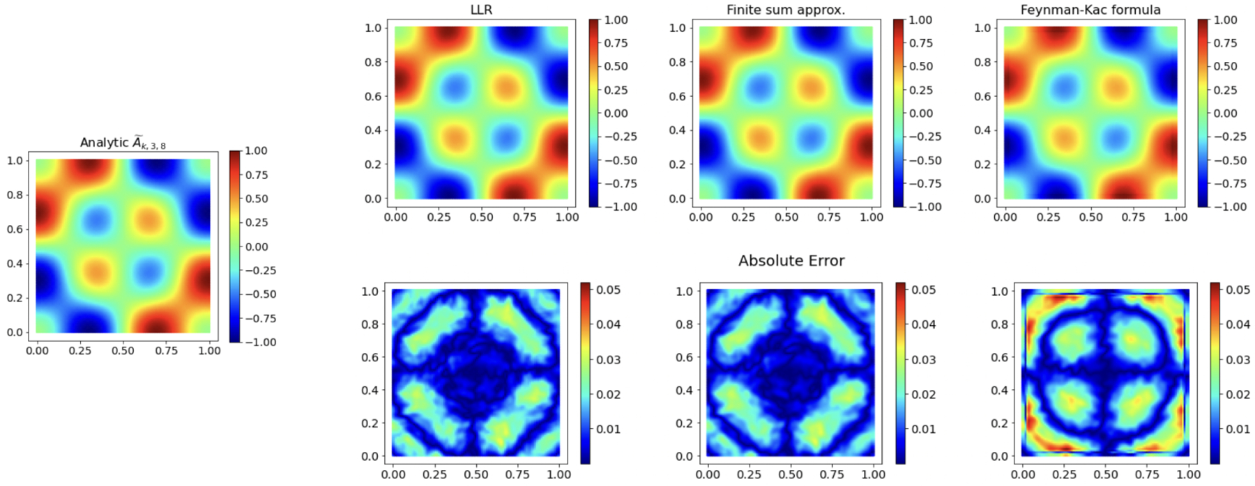
Comparison of different approaches to estimate ${\tilde{A}}_{kij}$ in the discrete setting.

Even though, in this example, the Feynman-Kac formulation seem to have a larger error, in our experiments, no single approach seem to be a clear winner across all the examples. This becomes clear in Appendix H where we provided a comparison of these approaches on a noiseless and a noisy Swiss Roll. The results shown in this paper are based on finite sum approximation to estimate ${\tilde{A}}_{kij}$.

3.3. Low Distortion Local Parameterization from Laplacian Eigenvectors

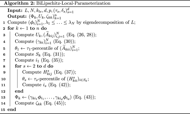
We use ∇ϕ_i ≡ ∇ϕ_i(x_k) for brevity. Using the estimates of ${\tilde{A}}_{kij}$, we now present an algorithmic construction of low distortion local parameterization Φ_k which maps U_k into ${ℝ}^d$. The pseudocode is provided below followed by a full explanation of the steps and a note on the hyperparameters. Before moving forward, it would be helpful for the reader to review the construction procedure in the continuous setting in Section 2.1.

An estimate of γ_ki is obtained by the discrete analog of Eq. (7) and is given by

$${\gamma }_{ki}=\text{Root-Mean-Square}{\left(\left\{{\varphi }_{ij}|x_j\in U_k\right\}\right)}^{-1}.$$ (30)

Step 1. Compute a set S_k of candidate eigenvectors for Φ_k.

Based on the construction procedure following Theorem 1, we start by computing a set S_k of candidate eigenvectors to construct Φ_k of U_k. There is no easy way to retrieve the set S_k in the discrete setting as in the procedure. Therefore, we make the natural choice of using the first N nontrivial eigenvectors ${\left({\varphi }_i\right)}_{i=1}^N$ of L corresponding to the N smallest eigenvalues ${\left({\lambda }_i\right)}_{i=1}^N$, with sufficiently large gradient at x_k, as the set S_k. The large gradient constraint is required for the numerical stability of our algorithm. Therefore, we set S_k to be,

$$S_k=\left\{i\in \left\{1,\dots .N\right\}|{‖\nabla {\varphi }_i‖}^2\ge {\theta }_1\right\}=\left\{i\in \left\{1,\dots ,N\right\}|{\tilde{A}}_{kii}\ge {\theta }_1\right\},$$ (31)

where θ₁ is ${\tau }_1$-percentile of the set ${\left({\tilde{A}}_{kii}\right)}_{i=1}^N$ and the second equality follows from Eq. (19). Here N and ${\tau }_1\in \left(0,100\right)$ are hyperparameters.

Step 2. Choose a direction $p_1\in T_{x_k}\mathcal{M}$.

The unit norm constraint on p₁ is relaxed. This will neither affect the math nor the output of our algorithm. Since p₁ can be arbitrary we take p₁ to be the gradient of an eigenvector r₁, that is $\nabla {\varphi }_{r_1}$. The choice of r₁ will determine ${\varphi }_{i_1}$. To obtain a low frequency eigenvector, r₁ is chosen so that the eigenvalue ${\lambda }_{r_1}$ is minimal, therefore

$$r_1=\underset{j\in S_k}{\text{argmin}}{\lambda }_j.$$ (32)

Step 3. Find i₁ ∈ S_k such that ${\gamma }_{k{i}_1}\left|\nabla {\varphi }_{i_1}^T{p}_1\right|$ is sufficiently large.

Since $p_1=\nabla {\varphi }_{r_1}$, using Eq. (19), the formula for $\nabla {\varphi }_i^T{p}_1$ becomes

$$\nabla {\varphi }_i^T{p}_1=\nabla {\varphi }_i^T\nabla {\varphi }_{r_1}={\tilde{A}}_{ki{r}_1}.$$ (33)

Then we obtain the eigenvector ${\varphi }_{i_1}$ so that ${\gamma }_{k{i}_1}\left|\nabla {\varphi }_{i_1}^T{p}_1\right|$ is larger than a certain threshold. We do not know what the value of this threshold would be in the discrete setting. Therefore, we first define the maximum possible value of ${\gamma }_{k{i}_1}\left|\nabla {\varphi }_i^T{p}_1\right|$ using Eq. (33) as

$${\alpha }_1=\underset{i\in S_k}{\max }{\gamma }_{ki}\left|\nabla {\varphi }_i^T{p}_1\right|=\underset{i\in S_k}{\max }{\gamma }_{ki}\left|{\tilde{A}}_{ki{r}_1}\right|.$$ (34)

Then we take the threshold to be δ₁α₁ where δ₁ ∈ (0,1] is a hyperparameter. Finally, to obtain a low frequency eigenvector ${\varphi }_{i_1}$, we choose i₁ such that

$$i_1=\underset{i\in S_k}{\text{argmin}}\left\{{\lambda }_i:{\gamma }_{ki}\left|\nabla {\varphi }_i^T{p}_1\right|\ge {\delta }_1{\alpha }_1\right\}=\underset{i\in S_k}{\text{argmin}}\left\{{\lambda }_i:{\gamma }_{ki}\left|{\tilde{A}}_{ki{r}_1}\right|\ge {\delta }_1{\alpha }_1\right\}.$$ (35)

After obtaining ${\varphi }_{i_1}$, we use a recursive procedure to obtain the s-th eigenvector ${\varphi }_{i_s}$ where s ∈ {2,...,d} in order.

Step 4. Choose a direction $p_s\in T_{x_k}\mathcal{M}$ orthogonal to $\nabla {\varphi }_{i_1},\dots ,\nabla {\varphi }_{i_s}$.

Again the unit norm constraint will be relaxed with no change in the output. We are going to take p_s to be the component of $\nabla {\varphi }_{r_s}$ orthogonal to $\nabla {\varphi }_{i_1},\dots ,\nabla {\varphi }_{i_s}$ for a carefully chosen r_s. For convenience, denote by V_s the matrix with $\nabla {\varphi }_{i_1},\dots ,\nabla {\varphi }_{i_{s-1}}$ as columns and let $\mathcal{R}\left(V_s\right)$ be the range of V_s. Let ${\varphi }_{r_s}$ be an eigenvector such that $\nabla {\varphi }_{r_s}\notin \mathcal{R}\left(V_s\right)$. To find such an r_s, we define

$$H_{kij}^s=\nabla {\varphi }_i^T\left(I-V_s{\left(V_s^T{V}_s\right)}^{-1}{V}_s^T\right)\nabla {\varphi }_j$$ (36)

$$={\tilde{A}}_{kij}-\left[{\tilde{A}}_{ki{i}_1}\dots {\tilde{A}}_{ki{i}_{s-1}}\right]{\left[\begin{array}{cccc}{\tilde{A}}_{k{i}_1{i}_1}& {\tilde{A}}_{k{i}_1{i}_2}& \dots & {\tilde{A}}_{k{i}_1{i}_{s-1}}\\ {\tilde{A}}_{k{i}_2{i}_1}& {\tilde{A}}_{k{i}_2{i}_2}& \dots & {\tilde{A}}_{k{i}_2{i}_{s-1}}\\ ⋮& ⋮& \ddots & ⋮\\ {\tilde{A}}_{k{i}_{s-1}{i}_1}& {\tilde{A}}_{k{i}_{s-1}{i}_2}& \dots & {\tilde{A}}_{k{i}_{s-1}{i}_{s-1}}\end{array}\right]}^{-1}\left[\begin{array}{c}{\tilde{A}}_{k{i}_{1}j}\\ {\tilde{A}}_{k{i}_{2}j}\\ ⋮\\ {\tilde{A}}_{k{i}_{s-1}j}\end{array}\right]$$ (37)

Note that $H_{kii}^s$ is the squared norm of the projection of ∇ϕ_i onto the vector space orthogonal to $\mathcal{R}\left(V_s\right)$. Clearly $\nabla {\varphi }_i\notin \mathcal{R}\left(V_s\right)$ if and only if $H_{kii}^s>0$. To obtain a low frequency eigenvector ${\varphi }_{r_s}$ such that $H_{k{r}_s{r}_s}^s>0$ we choose

$$r_s=\underset{i\in S_k}{\text{argmin}}\left\{{\lambda }_i:H_{kii}^s\ge {\theta }_s\right\}$$ (38)

where θ_s is the ${\tau }_s$-percentile of the set $\left\{H_{kii}^s:i\in S_k\right\}$ and ${\tau }_s\in \left(0,100\right)$ is a hyperparameter. Then we take p_s to be the component of $\nabla {\varphi }_{r_s}$ which is orthogonal to $\mathcal{R}\left(V_s\right)$,

$$p_s=\left(I-V_s{\left(V_s^T{V}_s\right)}^{-1}{V}_s^T\right)\nabla {\varphi }_{r_s}.$$ (39)

Step 5. Find i_s ∈ S_k such that ${\gamma }_{k{i}_s}\left|\nabla {\varphi }_{i_s}^T{p}_s\right|$ is sufficiently large.

Using Eq. (36, 39), we note that

$$\nabla {\varphi }_i^T{p}_s=H_{ki{r}_s}^s.$$ (40)

To obtain ${\varphi }_{i_s}$ such that ${\gamma }_{k{i}_s}\left|\nabla {\varphi }_{i_s}^T{p}_s\right|$ is greater than a certain threshold, as in step 3, we first define the maximum possible value of ${\gamma }_{k{i}_s}\left|\nabla {\varphi }_i^T{p}_s\right|$ using Eq. (40) as,

$${\alpha }_s=\underset{i\in S_k}{\max }{\gamma }_{ki}\left|\nabla {\varphi }_i^T{p}_s\right|=\underset{i\in S_k}{\max }{\gamma }_{ki}\left|H_{ki{r}_s}^s\right|.$$ (41)

Then we take the threshold to be δ_sα_s where δ_s ∈ [0,1] is a hyperparameter. Finally, to obtain a low frequency eigenvector ${\varphi }_{i_s}$ we choose i_s such that

$$i_s=\underset{i\in S_k}{\text{argmin}}\left\{{\lambda }_i:{\gamma }_{ki}\left|\nabla {\varphi }_i^T{p}_s\right|\ge {\delta }_s{\alpha }_s\right\}=\underset{i\in S_k}{\text{argmin}}\left\{{\lambda }_i:{\gamma }_{ki}\left|H_{ki{r}_s}^s\right|\ge {\delta }_s{\alpha }_s\right\}.$$ (42)

In the end we obtain a d-dimensional parameterization Φ_k of U_k given by

$$\begin{array}{l}\hspace{0.17em}\hspace{0.17em} \hspace{0.17em}\hspace{0.17em}\hspace{0.17em}\hspace{0.17em}\hspace{0.17em}\hspace{0.17em}\hspace{0.17em}\hspace{0.17em}{\mathrm{\Phi }}_k\equiv \left({\gamma }_{k{i}_1}{\varphi }_{i_1},\dots ,{\gamma }_{k{i}_d}{\varphi }_{i_d}\right)\hspace{0.33em}\text{where}\\ {\mathrm{\Phi }}_k\left(x_{k^{\prime }}\right)=\left({\gamma }_{k{i}_1}{\varphi }_{i_1{k}^{\prime }},\dots ,{\gamma }_{k{i}_d}{\varphi }_{i_d{k}^{\prime }}\right)\hspace{0.33em}\text{and}\\ {\mathrm{\Phi }}_k\left(U_k\right)={\left({\mathrm{\Phi }}_k\left(x_{k^{\prime }}\right)\right)}_{x_{k^{\prime }}\in U_k}.\end{array}$$ (43)

We call Φ_k(U_k) the kth local view of the data in the d-dimensonal embedding space. It is a matrix with |U_k| rows and d columns. Denote the distortion of ${\mathrm{\Phi }}_{k^{\prime }}$ on U_k by ${\zeta }_{k{k}^{\prime }}$. Using Eq. (1) we obtain

$${\zeta }_{k{k}^{\prime }}=\text{Distortion}\left({\mathrm{\Phi }}_{k^{\prime }},U_k\right)$$ (44)

$$=\underset{\begin{array}{c}{x}_l,x_{l^{\prime }}\in U_k\\ x_l\ne x_{l^{\prime }}\end{array}}{\sup }\frac{‖{\mathrm{\Phi }}_{k^{\prime }}\left(x_l\right)-{\mathrm{\Phi }}_{k^{\prime }}\left(x_{l^{\prime }}\right)‖}{d_e\left(x_l,x_{l^{\prime }}\right)}\underset{\begin{array}{c}{x}_l,x_{l^{\prime }}\in U_k\\ x_l\ne x_{l^{\prime }}\end{array}}{\sup }\frac{d_e\left(x_l,x_{l^{\prime }}\right)}{‖{\mathrm{\Phi }}_{k^{\prime }}\left(x_l\right)-{\mathrm{\Phi }}_{k^{\prime }}\left(x_{l^{\prime }}\right)‖}.$$ (45)

Postprocessing.

The obtained local parameterizations are post-processed so as to remove the anomalous parameterizations having unusually high distortion. We replace the local parameterization Φ_k of U_k by that of a neighbor, ${\mathrm{\Phi }}_{k^{\prime }}$ where $x_{k^{\prime }}\in U_k$, if the distortion ${\zeta }_{k{k}^{\prime }}$ produced by ${\mathrm{\Phi }}_{k^{\prime }}$ on U_k is smaller than the distortion ζ_kk produced by Φ_k on U_k. If ${\zeta }_{k{k}^{\prime }}<{\zeta }_{kk}$ for multiple k^′ then we choose the parameterization which produces the least distortion on U_k. This procedure is repeated until no replacement is possible. The pseudocode is provided below.

A note on hyperparameters N,${\left({\tau }_s,{\delta }_s\right)}_{s=1}^d$.

Generally, N should be small so that the low frequency eigenvectors form the set of candidate eigenvectors. In almost all of our experiments we take N to be 100. The set of ${\left({\tau }_s,{\delta }_s\right)}_{s=1}^d$ is reduced to two hyperparameters, one for all ${\tau }_s$‘s and one for all δ_s’s. As explained above, ${\tau }_s$ enforces certain vectors to be non-zero and δ_s enforces certain directional derivatives to be large enough. Therefore, a small value of ${\tau }_s$ in (0, 100) and a large value of δ_s in (0, 1] is suitable. In most of our experiments, we used a value of 50 for all ${\tau }_s$ and a value of 0.9 for all δ_s. Our algorithm is not too sensitive to the values of these hyperparameters. Other values of N, ${\tau }_s$ and δ_s would also result in the embeddings with high visual quality.

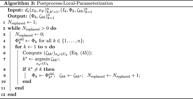
Example. We now build upon the example of the square grid at the end of Section 3.2. The values of the additional inputs are N = 100, ${\tau }_s=50$ and δ_s = 0.9 for all s ∈ {1,...,d}. Using Algo. 2 and 3 we obtain 10⁴ local views U_k and Φ_k(U_k) where |U_k| = 25 for all k. In the left image of Figure 5, we colored each point x_k with the distortion ζ_kk of the local parameterization Φ_k on U_k. The mapped discrete balls Φ_k(U_k) for some values of k are also shown in Figure 30 in the Appendix H.

Figure 5:

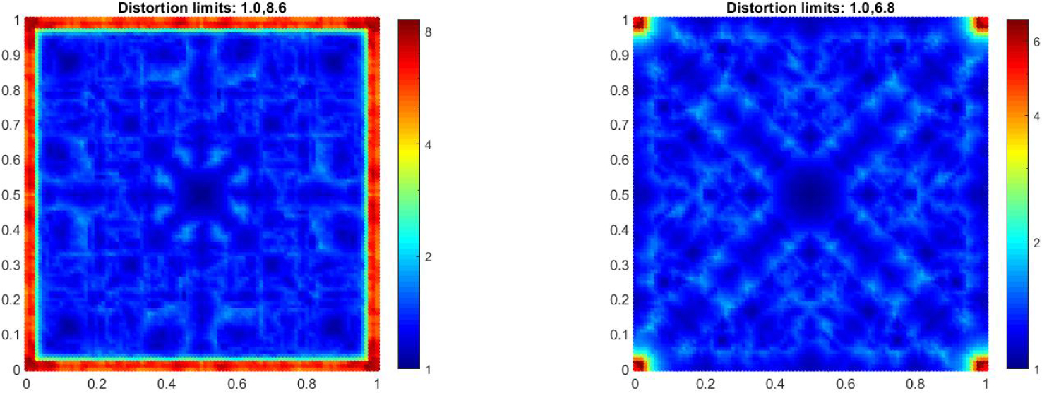
Distortion of the obtained local parameterizations when the points on the boundary are not known (left) versus when they are known apriori (right). Each point x_k is colored by ζ_kk (see Eq. (45)).

Remark 4. Note that the parameterizations of the discrete balls close to the boundary have higher distortion. This is because the injectivity radius at the points close to the boundary is low and precisely zero at the points on the boundary. As a result, the size of the balls around these points exceeds the limit beyond which Theorem 1 is applicable.

At this point we note the following remark in (Jones et al., 2007).

Remark 5. As was noted by L. Guibas, when M has a boundary, in the case of Neumann boundary values, one may consider the “doubled” manifold, and may apply the result in Theorem 1 for a possibly larger r_k.

Due to the above remark, assuming that the points on the boundary are known, we computed the distance matrix for the doubled manifold using the method described in (Lafon, 2004). Then we recomputed the local parameterizations Φ_k keeping all other hyperparameters the same as before. In the right image of Figure 5, we colored each point x_k with the distortion of the updated parameterization Φ_k on U_k. Note the reduction in the distortion of the paramaterizations for the neighborhoods close to the boundary. The distortion is still high near the corners.

3.4. Time Complexity

The combined worst case time complexity of Algo. 1, 2 and 3 is $O\left(n\left(N^2\left(k_{\text{lv}}+d\right)+k_{\text{lv}}^3{N}_{\text{post}}d\right)\right)$ where N_post is the number of iterations it takes to converge in Algo. 3 which was observed to be less than 50 for all the examples in this paper. It took about a minute¹ to construct the local views in the above example as well as in all the examples in Section 6.

4. Clustering for Intermediate Views

Recall that the discrete balls U_k are the local views of the data in the high dimensional ambient space. In the previous section, we obtained the mappings Φ_k to construct the local views Φ_k(U_k) of the data in the d-dimensional embedding space. As discussed in Section 1.2, one can use the GPA (Crosilla and Beinat, 2002; Gower, 1975; Ten Berge, 1977) to register these local views to recover a global embedding. In practice, too many small local views (high n and small |U_k|) result in extremely high computational complexity. Moreover, small overlaps between the local views makes their registration susceptible to errors. Therefore, we perform clustering to obtain M ≪ n intermediate views, ${\tilde{U}}_m$ and ${\tilde{\mathrm{\Phi }}}_m\left({\tilde{U}}_m\right)$, of the data in the ambient space and the embedding space, respectively. This reduces the time complexity and increases the overlaps between the views, leading to their quick and robust registration.

4.1. Notation

Our clustering algorithm is designed so as to ensure low distortion of the parameterizations ${\tilde{\mathrm{\Phi }}}_m$ on ${\tilde{U}}_m$. We first describe the notation used and then present the pseudocode followed by a full explanation of the steps. Let c_k be the index of the cluster x_k belongs to. Then the set of points which belong to cluster m is given by

$${\mathcal{C}}_m=\left\{x_k|c_k=m\right\}.$$ (46)

Denote by $c_{U_k}$ the set of indices of the neighboring clusters of x_k. The neighboring points of x_k lie in these clusters, that is,

$$c_{U_k}=\left\{c_{k^{\prime }}|x_{k^{\prime }}\in U_k\right\}.$$ (47)

We say that a point x_k lies in the vicinity of a cluster m if $m\in c_{U_k}$. Let ${\tilde{U}}_m$ denote the mth intermediate view of the data in the ambient space. This constitutes the union of the local views associated with all the points belonging to cluster m, that is,

$${\tilde{U}}_m={\displaystyle \underset{k:\hspace{0.33em}{x}_k\in {\mathcal{C}}_m}{\cup }{U}_k}.$$ (48)

Clearly, a larger cluster means a larger intermediate view. In particular, addition of x_k to ${\mathcal{C}}_m$ grows the intermediate view ${\tilde{U}}_m$ to ${\tilde{U}}_m\cup U_k$,

$${\mathcal{C}}_m\to {\mathcal{C}}_m\cup \left\{x_k\right\}\Rightarrow {\tilde{U}}_m\to {\tilde{U}}_m\cup U_k$$ (49)

Let ${\tilde{\Phi }}_m$ be the d-dimensional parameterization associated with the mth cluster. This parameterization maps ${\tilde{U}}_m$ to ${\tilde{\Phi }}_m\left({\tilde{U}}_m\right)$, the mth intermediate view of the data in the embedding space. Note that a point x_k generates the local view U_k (see Eq. (26)) which acts as the domain of the parameterization Φ_k. Similarly, a cluster ${\mathcal{C}}_m$ obtained through our procedure, generates an intermediate view ${\tilde{U}}_m$ (see Eq. (48)) which acts as the domain of the parameterization${\tilde{\Phi }}_m$. Overall, our clustering procedure replaces the notion of a local view per an individual point by an intermediate view per a cluster of points.

4.2. Low Distortion Clustering

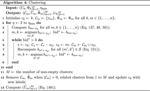
Initially, we start with n singleton clusters where the point x_k belongs to the kth cluster and the parameterization associated with the kth cluster is Φ_k. Thus, c_k = k, ${\mathcal{C}}_m=\left\{x_m\right\}$ and ${\tilde{\mathrm{\Phi }}}_m={\mathrm{\Phi }}_m$ for all k,m ∈ {1,...,n}. This automatically implies that initially ${\tilde{U}}_m=U_m$. The parameterizations associated with the clusters remain the same throughout the procedure. During the procedure, each cluster ${\mathcal{C}}_m$ is perceived as an entity which wants to grow the domain ${\tilde{U}}_m$ of the associated parameterization ${\tilde{\mathrm{\Phi }}}_m$ by growing itself (see Eq. 49), while simultaneously keeping the distortion of ${\tilde{\mathrm{\Phi }}}_m$ on ${\tilde{U}}_m$ low (see Eq. 45). To achieve that, each cluster ${\mathcal{C}}_m$ places a careful bid $b_{m\leftarrow x_k}$ for each point x_k. The global maximum bid is identified and the underlying point x_k is relabelled to the bidding cluster, hence updating c_k. With this relabelling, the bidding cluster grows and the source cluster shrinks. This procedure of shrinking and growing clusters is repeated until all non-empty clusters are large enough, i.e. have a size at least η_min, a hyperparameter. In our experiments, we choose η_min from {5,10,15,20,25}. We iterate over η which varies from 2 to η_min.

In the η-th iteration, we say that the mth cluster is small if it is non-empty and has a size less than η, that is, when $\left|{\mathcal{C}}_m\right|\in \left(0,\eta \right)$. During the iteration, the clusters either shrink or grow until no small clusters remain. Therefore, at the end of the η-th iteration the non-empty clusters are of size at least η. After the last (η_minth) iteration, each non-empty cluster will have at least η_min points and the empty clusters are pruned away.

Bid by cluster m for x_k.

In the η-th iteration, we start by computing the bid $b_{m\leftarrow x_k}$ by each cluster m for each point x_k. The bid function is designed so as to satisfy the following conditions. The first two conditions are there to halt the procedure while the last two conditions follow naturally. These conditions are also depicted in Figure 6.

Figure 6:

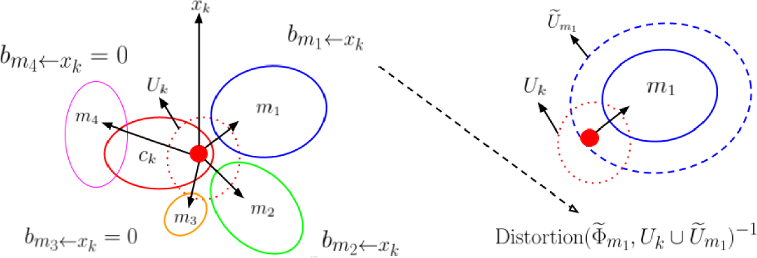
Computation of the bid for a point in a small cluster by the neighboring clusters in η-th iteration. (left) x_k is a point represented by a small red disc, in a small cluster c_k enclosed by solid red line. The dashed red line enclose U_k. Assume that the cluster c_k is small so that $\left|{\mathcal{C}}_{c_k}\right|\in \left(0,\eta \right)$. Clusters m₁, m₂, m₃ and m₄ are enclosed by solid colored lines too. Note that m₁, m₂ and m₃ lie in $c_{U_k}$ (the nonempty overlap between these clusters and U_k indicate that), while $m_4\notin c_{U_k}$. Thus, the bid by m₄ for x_k is zero. Since the size of cluster m₃ is less than the size of cluster c_k i.e.$\left|{\mathcal{C}}_{m_3}\right|<\left|{\mathcal{C}}_{c_k}\right|$, the bid by m₃ for x_k is also zero. Since clusters m₁ and m₂ satisfy all the conditions, the bids by m₁ and m₂ for x_k are to be computed. (right) The bid $b_{m_1\leftarrow x_k}$, is given by the inverse of the distortion of ${\tilde{\mathrm{\Phi }}}_{m_1}$ on $U_k\cup {\tilde{U}}_{m_1}$, where the dashed blue line enclose ${\tilde{U}}_{m_1}$. If the bid $b_{m_1\leftarrow x_k}$ is greater (less) than the bid $b_{m_2\leftarrow x_k}$, then the clustering procedure would favor relabelling of x_k to m₁ (m₂).

1. No cluster bids for the points in large clusters. Since x_k belongs to cluster c_k therefore, if $\left|{\mathcal{C}}_{c_k}\right|>\eta$ then the $b_{m\leftarrow x_k}$ is zero for all m.

2. No cluster bids for a point in another cluster whose size is bigger than its own size. Therefore, if $\left|{\mathcal{C}}_m\right|<\left|{\mathcal{C}}_{c_k}\right|$ then again $b_{m\leftarrow x_k}$ is zero.

3. A cluster bids for the points in its own vicinity. Therefore, if $m\notin c_{U_k}$ (see Eq. 47) then $b_{m\leftarrow x_k}$ is zero.

4. Recall that a cluster m aims to grow while keeping the distortion of associated parameterization ${\tilde{\mathrm{\Phi }}}_m$ low on its domain ${\tilde{U}}_m$. If the mth cluster acquires the point x_k, ${\tilde{U}}_m$ grows due to the addition of U_k to it (see Eq. (48)), and so does the distortion of ${\tilde{\mathrm{\Phi }}}_m$ on it. Therefore, to ensure low distortion, the natural bid by ${\mathcal{C}}_m$ for the point x_k, $b_{m\leftarrow x_k}$, is Distortion ${\left({\tilde{\mathrm{\Phi }}}_m,U_k\cup {\tilde{U}}_m\right)}^{-1}$ (see Eq. 45).

Combining the above conditions, we can write the bid by cluster m for the point x_k as,

$$b_{m\leftarrow x_k}=\left\{\begin{array}{c}\text{Distortion}{\left({\tilde{\Phi }}_m,U_k\cup {\tilde{U}}_m\right)}^{-1}\\ 0\end{array}\hspace{1em}\begin{array}{c}\text{if}\hspace{0.33em}\left|{\mathcal{C}}_{c_k}\right|\in \left(0,\eta \right)\wedge m\in c_{U_k}\wedge \left|{\mathcal{C}}_m\right|\ge \left|{\mathcal{C}}_{c_k}\right|\\ \text{otherwise}.\end{array}\right.$$ (50)

In the practical implementation of above equation, $c_{U_k}$ and ${\tilde{U}}_m$ are computed on the fly using Eq. (47, 48).

Greedy procedure to grow and shrink clusters.

Given the bids by all the clusters for all the points, we grow and shrink the clusters so that at the end of the current iteration η, each non-empty cluster has a size at least η. We start by picking the global maximum bid, say $b_{m\leftarrow x_k}$. Let x_k be in the cluster s (note that c_k, the cluster of x_k, is s before x_k is relabelled). We relabel c_k to m, and update the set of points in clusters s and m, ${\mathcal{C}}_s$ and ${\mathcal{C}}_m$, using Eq. (46). This implicitly shrinks ${\tilde{U}}_s$ and grows ${\tilde{U}}_m$ (see Eq. 48) and affects the bids by clusters m and s or the bids for the points in these clusters. Denote the set of pairs of the indices of all such clusters and the points by

$$\mathcal{S}=\left\{\left(m^{\prime },k^{\prime }\right)\in {\left\{1,\dots ,n\right\}}^2|m^{\prime }\in \left\{m,s\right\}\hspace{0.33em}\text{or}\hspace{0.33em}{x}_{k^{\prime }}\in {\mathcal{C}}_s\cup {\mathcal{C}}_m\right\}.$$ (51)

Then the bids $b_{m^{\prime }\leftarrow x_{k^{\prime }}}$ are recomputed for all $\left(m^{\prime },k^{\prime }\right)\in \mathcal{S}$. It is easy to verify that for all other pairs, neither the conditions nor the distortion in Eq. (50) are affected. After this computation, we again pick the global maximum bid and repeat the procedure until the maximum bid becomes zero indicating that no non-empty small cluster remains. This marks the end of the η-th iteration.

Final intermediate views in the ambient and the embedding space.

At the end of the last iteration, all non-empty clusters have at least η_min points. Let M be the number of non-empty clusters. Using the pigeonhole principle one can show that M would be less than or equal to n/η_min. We prune away the empty clusters and relabel the non-empty ones from 1 to M while updating c_k accordingly. With this, we obtain the clusters ${\left({\mathcal{C}}_m\right)}_{m=1}^M$ with associated parameterizations ${\left({\tilde{\mathrm{\Phi }}}_m\right)}_{m=1}^M$. Finally, using Eq. (48), we obtain the M intermediate views ${\left({\tilde{U}}_m\right)}_{m=1}^M$ of the data in the ambient space. Then, the intermediate views of the data in the embedding space are given by ${\left({\tilde{\mathrm{\Phi }}}_m\left({\tilde{U}}_m\right)\right)}_{m=1}^M$. Note that ${\tilde{\mathrm{\Phi }}}_m\left({\tilde{U}}_m\right)$ is a matrix with $\left|{\tilde{U}}_m\right|$ rows and d columns (see Eq. (43)).

Example. We continue with our example of the square grid which originally contained about 10⁴ points. Therefore, before clustering we had about 10⁴ small local views U_k and Φ_k(U_k), each containing 25 points. After clustering with η_min = 10, we obtained 635 clusters and therefore that many intermediate views ${\tilde{U}}_m$ and ${\tilde{\mathrm{\Phi }}}_m\left({\tilde{U}}_m\right)$ with an average size of 79. When the points on the boundary are known then we obtained 562 intermediate views with an average size of 90. Note that there is a trade-off between the size of the intermediate views and the distortion of the parameterizations used to obtain them. For convenience, define ${\tilde{\zeta }}_{mm}$ to be the distortion of ${\tilde{\mathrm{\Phi }}}_m$ on ${\tilde{U}}_m$ using Eq. (45). Then, as the size of the views are increased (by increasing η_min), the value of ${\tilde{\zeta }}_{mm}$ would also increase. In Figure 7 we colored the points in cluster m, ${\mathcal{C}}_m$, with ${\tilde{\zeta }}_{mm}$. In other words, x_k is colored by ${\tilde{\zeta }}_{c_k{c}_k}$. Note the increased distortion in comparison to Figure 5.

Figure 7:

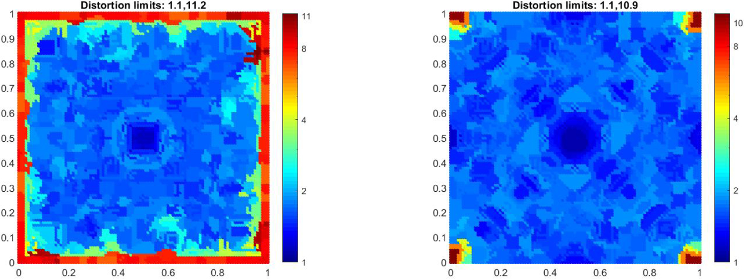
Each point x_k colored by ${\tilde{\zeta }}_{c_k{c}_k}$ when the points on the boundary of the square grid are unknown (left) versus when they are known apriori (right).

4.3. Time Complexity

Our practical implementation of Algo. 4 uses memoization for speed up. It took about a minute to construct intermediate views using in the above example with n = 10⁴, k_lv = 25, d = 2 and η_min = 10, and it took less than 2 minutes for all the examples in Section 6. It was empirically observed that the time for clustering is linear in n, η_min and d while it is cubic in k_lv.

5. Global Embedding using Procrustes Analysis

In this section, we present an algorithm based on Procrustes analysis to align the intermediate views ${\tilde{\mathrm{\Phi }}}_m\left({\tilde{U}}_m\right)$ and obtain a global embedding. The M views ${\tilde{\mathrm{\Phi }}}_m\left({\tilde{U}}_m\right)$ are transformed by an orthogonal matrix T_m of size d × d, a d-dimensional translation vector v_m and a positive scalar b_m as a scaling component. The transformed views are given by ${\tilde{\mathrm{\Phi }}}_m^g\left({\tilde{U}}_m\right)$ such that

$${\tilde{\mathrm{\Phi }}}_m^g\left(x_k\right)=b_m{\tilde{\mathrm{\Phi }}}_m\left(x_k\right)T_m+v_m\hspace{1em}\text{for}\hspace{0.33em}\text{all}\hspace{0.33em}{x}_k\in {\tilde{U}}_m.$$ (52)

First we state a general approach to estimate these parameters, and its limitations in Section 5.1. Then we present an algorithm in Section 5.2 which computes these parameters and a global embedding of the data while addressing the limitations of the general procedure. In Section 5.3 we describe a simple modification to our algorithm to tear apart closed manifolds. In Appendix F, we contrast our global alignment procedure with that of LTSA.

5.1. General Approach for Alignment

In general, the parameters ${\left(T_m,v_m,b_m\right)}_{m=1}^M$ are estimated so that for all m and m^′, the two transformed views of the overlap between ${\tilde{U}}_m$ and ${\tilde{U}}_{m^{\prime }}$, obtained using the parameterizations ${\tilde{\mathrm{\Phi }}}_m^g$ and ${\tilde{\mathrm{\Phi }}}_{m^{\prime }}^g$, align with each other. To be more precise, define the overlap between the mth and the m^′th intermediate views in the ambient space as the set of points which lie in both the views,

$${\tilde{U}}_{m{m}^{\prime }}={\tilde{U}}_m\cap {\tilde{U}}_{m^{\prime }}.$$ (53)

In the ambient space, the mth and the m^′th views are neighbors if ${\tilde{U}}_{m{m}^{\prime }}$ is non-empty. As shown in Figure 8 (left), these neighboring views trivially align on the overlap between them. It is natural to ask for a low distortion global embedding of the data. Therefore, we must ensure that the embeddings of ${\tilde{U}}_{m{m}^{\prime }}$ due to the mth and the m^′th view in the embedding space, also align with each other. Thus, the parameters ${\left(T_m,v_m,b_m\right)}_{m=1}^M$ are estimated so that ${\tilde{\mathrm{\Phi }}}_m^g\left({\tilde{U}}_{m{m}^{\prime }}\right)$ aligns with ${\tilde{\mathrm{\Phi }}}_{m^{\prime }}^g\left({\tilde{U}}_{m{m}^{\prime }}\right)$ for all m and m^′. However, due to the distortion of the parameterizations it is usually not possible to perfectly align the two embeddings (see Figure 8). We can represent both embeddings of the overlap as matrices with $\left|{\tilde{U}}_{m{m}^{\prime }}\right|$ rows and d columns. Then we choose the measure of the alignment error to be the squared Frobenius norm of the difference of the two matrices. The error is trivially zero if ${\tilde{U}}_{m{m}^{\prime }}$ is empty. Overall, the parameters are estimated so as to minimize the following alignment error

$$\mathcal{L}\left({\left(T_m,v_m,b_m\right)}_{m=1}^M\right)=\frac{1}{2M}{\displaystyle \sum _{\begin{array}{c}m=1\\ m^{\prime }=1\end{array}}^M{‖{\tilde{\mathrm{\Phi }}}_m^g\left({\tilde{U}}_{m{m}^{\prime }}\right)-{\tilde{\mathrm{\Phi }}}_{m^{\prime }}^g\left({\tilde{U}}_{m{m}^{\prime }}\right)‖}_F^2}.$$ (54)

In theory, one can start with a trivial initialization of T_m, v_m and b_m as I_d, 0 and 1, and directly use GPA (Crosilla and Beinat, 2002; Gower, 1975; Ten Berge, 1977) to obtain a local minimum of the above alignment error. This approach has two issues.

Figure 8:

(left) The intermediate views ${\tilde{U}}_m$ and ${\tilde{U}}_{m^{\prime }}$ of a 2d manifold in a possibly high dimensional ambient space. These views trivially align with each other. The red star in blue circles represent their overlap ${\tilde{U}}_{m{m}^{\prime }}$. (middle) The mth and m^′th intermediate views in the 2d embedding space. (right) Transformed views after aligning ${\tilde{\mathrm{\Phi }}}_m\left({\tilde{U}}_{m{m}^{\prime }}\right)$ with ${\tilde{\mathrm{\Phi }}}_{m^{\prime }}\left({\tilde{U}}_{m{m}^{\prime }}\right)$.

1. Like most optimization algorithms, the rate of convergence to a local minimum and the quality of it depends on the initialization of the parameters. We empirically observed that with a trivial initialization of the parameters, GPA may take a great amount of time to converge and may also converge to an inferior local minimum.

2. Using GPA to align a view with all of its adjacent views would prevent us from tearing apart closed manifolds; as an example see Figure 11.

Figure 11:

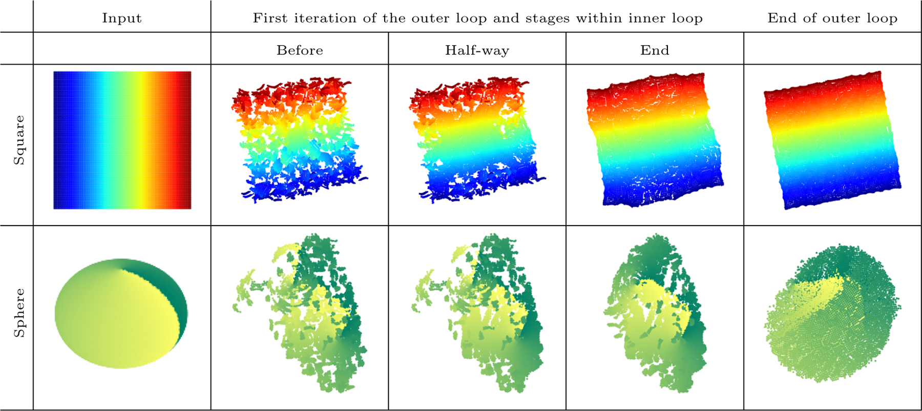
2d embeddings of a square and a sphere at different stages of Algo. 5. For illustration purpose, in the plots in the 2nd and 3rd columns the translation parameter v_m was manually set for those views which do not lie in the set $\mathcal{A}$. Note that the embedding of the sphere is fallacious. The reason and the resolution is provided in Section 5.3.

These issues are addressed in subsequent Sections 5.2 and 5.3, respectively.

5.2. GPA Adaptation for Global Alignment

First we look for a better than trivial initialization of the parameters so that the views are approximately aligned. The idea is to build a rooted tree where nodes represent the intermediate views. This tree is then traversed in a breadth first order starting from the root. As we traverse the tree, the intermediate view associated with a node is aligned with the intermediate view associated with its parent node (and with a few more views), thus giving a better initialization of the parameters. Subsequently, we refine these parameters using a similar procedure involving random order traversal over the intermediate views.

Initialization (Iter = 1, to tear = False).

In the first outer loop of Algo. 5, we start with T_m = I_d, v_m as the zero vector and compute b_m so as to bring the intermediate views ${\tilde{\mathrm{\Phi }}}_m\left({\tilde{U}}_m\right)$ to the same scale as their counterpart ${\tilde{U}}_m$ in the ambient space. In turn this brings all the views to similar scale (see Figure 9 (c)). We compute the scaling component b_m to be the ratio of the median distance between unique points in ${\tilde{U}}_m$ and in ${\tilde{\mathrm{\Phi }}}_m\left({\tilde{U}}_m\right)$, that is,

$$b_m=\frac{\text{median}\left\{d_e\left(x_k,x_{k^{\prime }}\right)|x_k,x_{k^{\prime }}\in {\tilde{U}}_m,x_k\ne x_{k^{\prime }}\right\}}{\text{median}\left\{{‖{\tilde{\mathrm{\Phi }}}_m\left(x_k\right)-{\tilde{\mathrm{\Phi }}}_m\left(x_{k^{\prime }}\right)‖}_2|x_k,x_{k^{\prime }}\in {\tilde{U}}_m,x_k\ne x_{k^{\prime }}\right\}}.$$ (55)

Then we transform the the views in a sequence ${\left(s_m\right)}_{m=1}^M$. This sequence corresponds to the breadth first ordering of a tree starting from its root node (which represents s₁th view). Let the $p_{s_m}$ th view be the parent of the s_mth view. Here $p_{s_m}$ lies in {s₁,...,s_m−1} and it is a neighboring view of the s_mth view in the ambient space, i.e. ${\tilde{U}}_{s_m{p}_{s_m}}$ is non-empty. Details about the computation of these sequences is provided in Appendix D. Note that $p_{s_1}$ is not defined and consequently, the first view in the sequence (s₁th view) is not transformed, therefore $T_{s_1}$ and $v_{s_1}$ are not updated. We also define $\mathcal{A}$, initialized with s₁, to keep track of visited nodes which also represent the already transformed views. Then we iterate over m which varies from 2 to M. For convenience, denote the current (mth) node s_m by s and its parent $p_{s_m}$ by p. The following procedure updates T_s and v_s (refer to Figure 9 and 10 for an illustration of this procedure).

Figure 9:

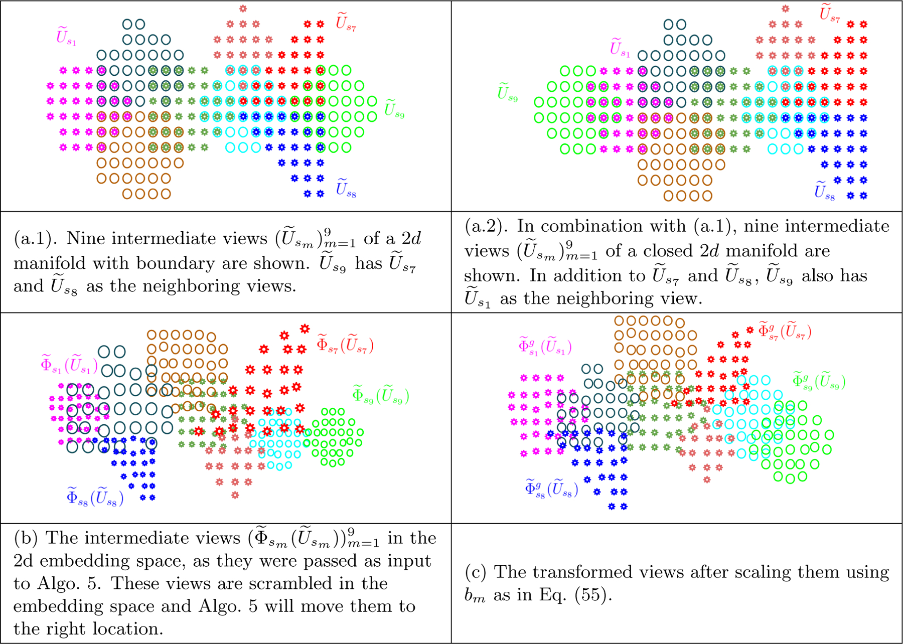
An illustration of the intermediate views in the ambient and the embedding space as they are passed as input to Algo. 5 and are scaled using Eq. (55).

Figure 10:

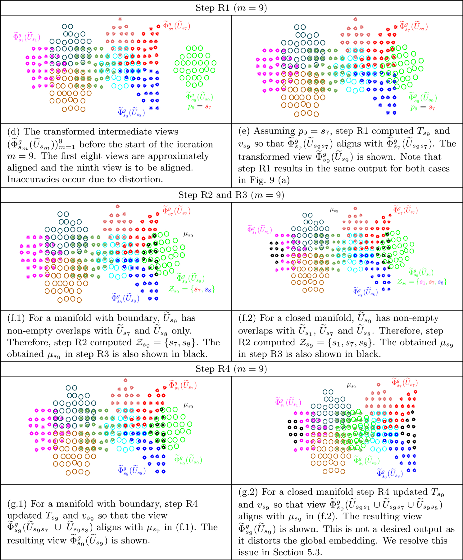
An illustration of steps R1 to R4 in Algo. 5, in continuation of Figure 9.

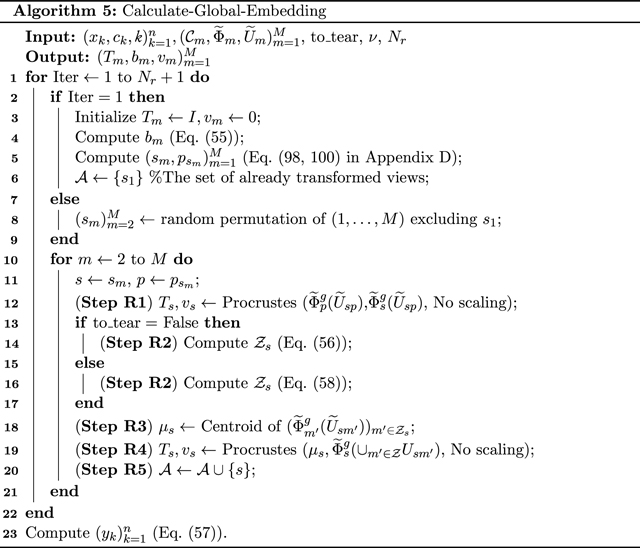
Step R1. We compute a temporary value of T_s and v_s by aligning the views ${\tilde{\mathrm{\Phi }}}_s^g\left({\tilde{U}}_{sp}\right)$ and ${\tilde{\mathrm{\Phi }}}_p^g\left({\tilde{U}}_{sp}\right)$ of the overlap ${\tilde{U}}_{sp}$, using Procrustes analysis (Gower et al., 2004) without modifying b_s.

Step R2. Then we identify more views to align the sth view with. We compute a subset ${\mathcal{Z}}_s$ of the set of already visited nodes $\mathcal{A}$ such that $m^{\prime }\in {\mathcal{Z}}_s$ if the sth view and the m^′th view are neighbors in the ambient space. Note that, at this stage, $\mathcal{A}$ is the same as the set {s₁,...,s_m−1}, the indices of the first m − 1 views. Therefore,

$${\mathcal{Z}}_s=\left\{m^{\prime }|{\tilde{U}}_{s{m}^{\prime }}\ne \cancel{0}\right\}\cap \mathcal{A}.$$ (56)

Step R3. We then compute the centroid µ_s of the views ${\left({\tilde{\mathrm{\Phi }}}_{m^{\prime }}^g\left({\tilde{U}}_{s{m}^{\prime }}\right)\right)}_{m^{\prime }\in {\mathcal{Z}}_s}$. Here µ_s is a matrix with d columns and the number of rows given by the size of the set ${\cup }_{m^{\prime }\in {\mathcal{Z}}_s}{\tilde{U}}_{s{m}^{\prime }}$. A point in this set can have multiple embeddings due to multiple parameterizations ${\left({\tilde{\mathrm{\Phi }}}_{m^{\prime }}^g\right)}_{m^{\prime }\in {\mathcal{Z}}_s}$ depending on the overlaps ${\left({\tilde{U}}_{s{m}^{\prime }}\right)}_{m^{\prime }\in {\mathcal{Z}}_s}$ it lies in. The mean of these embeddings forms a row in µ_s.

Step R4. Finally, we update T_s and v_s by aligning the view ${\tilde{\mathrm{\Phi }}}_s^g\left({\tilde{U}}_{s{m}^{\prime }}\right)$ with ${\tilde{\mathrm{\Phi }}}_{m^{\prime }}^g\left({\tilde{U}}_{s{m}^{\prime }}\right)$ for all $m^{\prime }\in {\mathcal{Z}}_s$. This alignment is based on the approach in (Crosilla and Beinat, 2002; Gower, 1975) where, using the Procrustes analysis (Gower et al., 2004; MATLAB, 2018), the view ${\tilde{\mathrm{\Phi }}}_s^g\left({\cup }_{m^{\prime }\in {\mathcal{Z}}_s}{\tilde{U}}_{s{m}^{\prime }}\right)$ is aligned with the centroid µ_s, without modifying b_s.

Step R5. After the sth view is transformed, we add it to the set of transformed views $\mathcal{A}$.

Parameter Refinement (Iter ≥ 2, to tear = False).

At the end of the first iteration of the outer loop in Algo. 5, we have an initialization of ${\left(T_m,b_m,v_m\right)}_{m=1}^M$ such that transformed intermediate views are approximately aligned. To further refine these parameters, we iterate over ${\left(s_m\right)}_{m=2}^M$ in random order and perform the same five step procedure as above, N_r times. Besides the random-order traversal, the other difference in a refinement iteration is that the set of already visited nodes $\mathcal{A}$, contains all the nodes instead of just the first m − 1 nodes. This affects the computation of ${\mathcal{Z}}_s$ (see Eq. (56)) in step R2 so that the sth intermediate view is now aligned with all those views which are its neighbors in the ambient space. Note that the step R5 is redundant during refinement.

In the end, we compute the global embedding y_k of x_k by mapping x_k using the transformed parameterization associated with the cluster c_k it belongs to,

$$y_k={\tilde{\mathrm{\Phi }}}_{c_k}^g\left(x_k\right).$$ (57)

An illustration of the global embedding at various stages of Algo. 5 is provided in Figure 11.

5.3. Tearing Closed Manifolds

When the manifold has no boundary, then the step R2 in above section may result in a set ${\mathcal{Z}}_s$ containing the indices of the views which are neighbors of the sth view in the ambient space but are far apart from the transformed sth view in the embedding space, obtained right after step R1. For example, as shown in Figure 10 (f.2), $s_1\in {\mathcal{Z}}_{s_9}$ because the s₉th view and the s₁th view are neighbors in the ambient space (see Figure 9 (a.1, a.2)) but in the embedding space, they are far apart. Due to such indices in ${\mathcal{Z}}_{s_9}$, the step R3 results in a centroid, which when used in step R4, results in a fallacious estimation of the parameters T_s and v_s, giving rise to a high distortion embedding. By trying to align with all its neighbors in the ambient space, the s₉th view is misaligned with respect to all of them (see Figure 10 (g.2)).

Resolution (to_tear = True).

We modify the step R2 so as to introduce a discontinuity by including the indices of only those views in the set ${\mathcal{Z}}_s$ which are neighbors of the sth view in both the ambient space as well as in the embedding space. We denote the overlap between the mth and m^′th view in the embedding space by ${\tilde{U}}_{m{m}^{\prime }}^g$. There may be multiple heuristics for computing ${\tilde{U}}_{m{m}^{\prime }}^g$ which could work. In the Appendix E, we describe a simple approach based on the already developed machinery in this paper, which uses the hyperparameter ν provided as input to Algo. 5. Having obtained ${\tilde{U}}_{m{m}^{\prime }}^g$, we say that the mth and the m^′th intermediate views in the embedding space are neighbors if ${\tilde{U}}_{m{m}^{\prime }}^g$ is non-empty.

Step R2. Finally, we compute ${\mathcal{Z}}_s$ as,

$${\mathcal{Z}}_s=\left\{m^{\prime }|{\tilde{U}}_{s{m}^{\prime }}\ne \cancel{0},\hspace{0.33em}{\tilde{U}}_{s{m}^{\prime }}^g\ne \cancel{0}\right\}\cap \mathcal{A}.$$ (58)

Note that if it is known apriori that the manifold can be embedded in lower dimension without tearing it apart then we do not require the above modification. In all of our experiments except the one in Section 6.5, we do not assume that this information is available.

With this modification, the set ${\mathcal{Z}}_{s_9}$ in Figure 10 (f.2) will not include s₁ and therefore the resulting centroid in the step R3 would be the same as the one in Figure 10 (f.1). Subsequently, the transformed s₉th view would be the one in Figure 10 (g.1) rather than Figure 10 (g.2).

Gluing instruction for the boundary of the embedding.

Having knowingly torn the manifold apart, we provide at the output, information on the points belonging to the tear and their neighboring points in the ambient space. To encode the “gluing” instructions along the tear in the form of colors at the output of our algorithm, we recompute ${\tilde{U}}_{m{m}^{\prime }}^g$. If ${\tilde{U}}_{m{m}^{\prime }}$ is non-empty but ${\tilde{U}}_{m{m}^{\prime }}^g$ is empty, then this means that the mth and m^′th views are neighbors in the ambient space but are torn apart in the embedding space. Therefore, we color the global embedding of the points on the overlap ${\tilde{U}}_{m{m}^{\prime }}$ which belong to clusters ${\mathcal{C}}_m$ and ${\mathcal{C}}_{m^{\prime }}$ with the same color to indicate that although these points are separated in the embedding space, they are adjacent in the ambient space (see Figures 19, 20 and 31).

Figure 19:

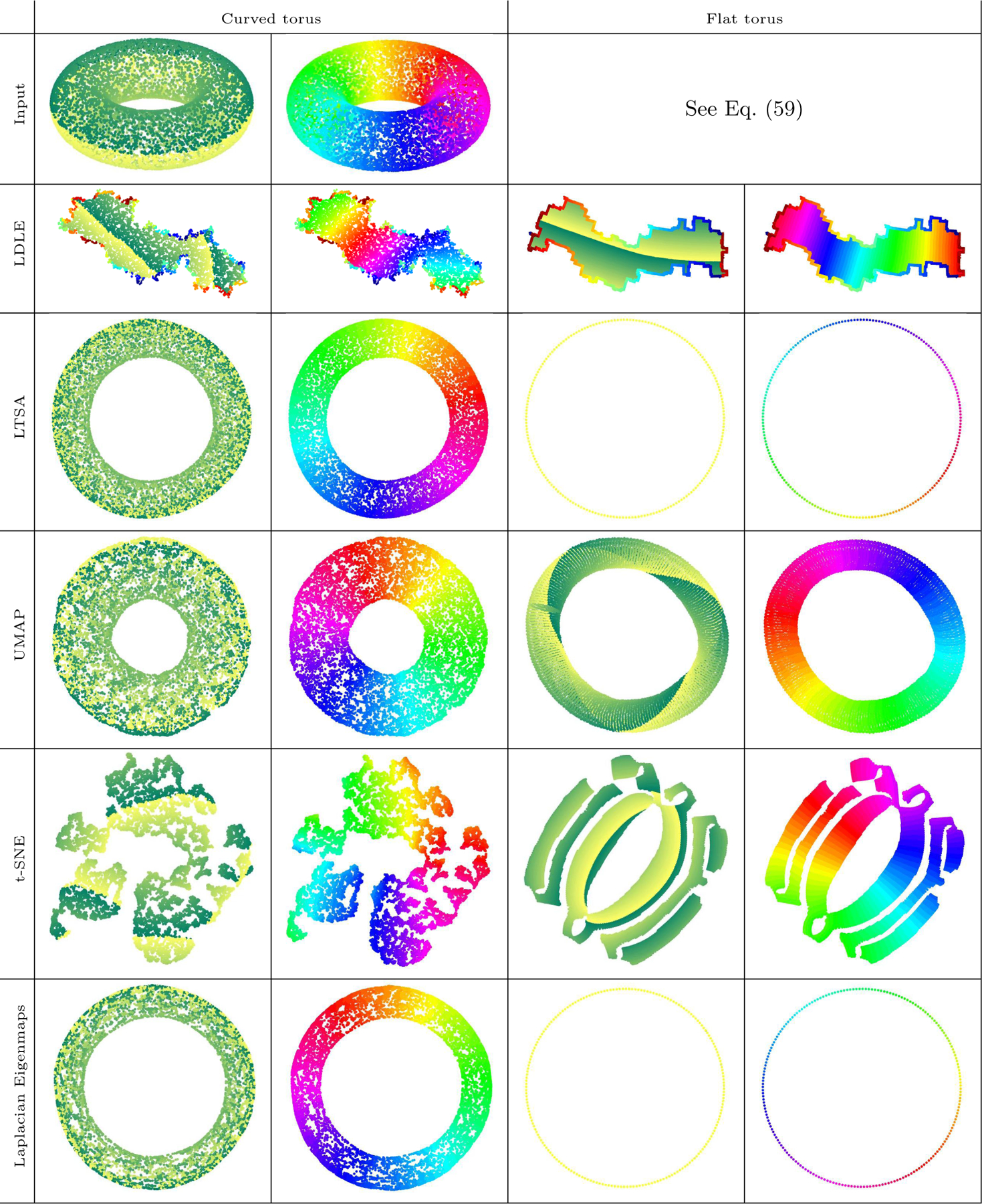
Embeddings of 2d manifolds without boundary into ${ℝ}^2$. For each manifold, the left and right columns contain the same plots colored by the two parameters of the manifold. A proof of the mathematical correctness of the LDLE embeddings is provided in Figure 31.

Figure 20:

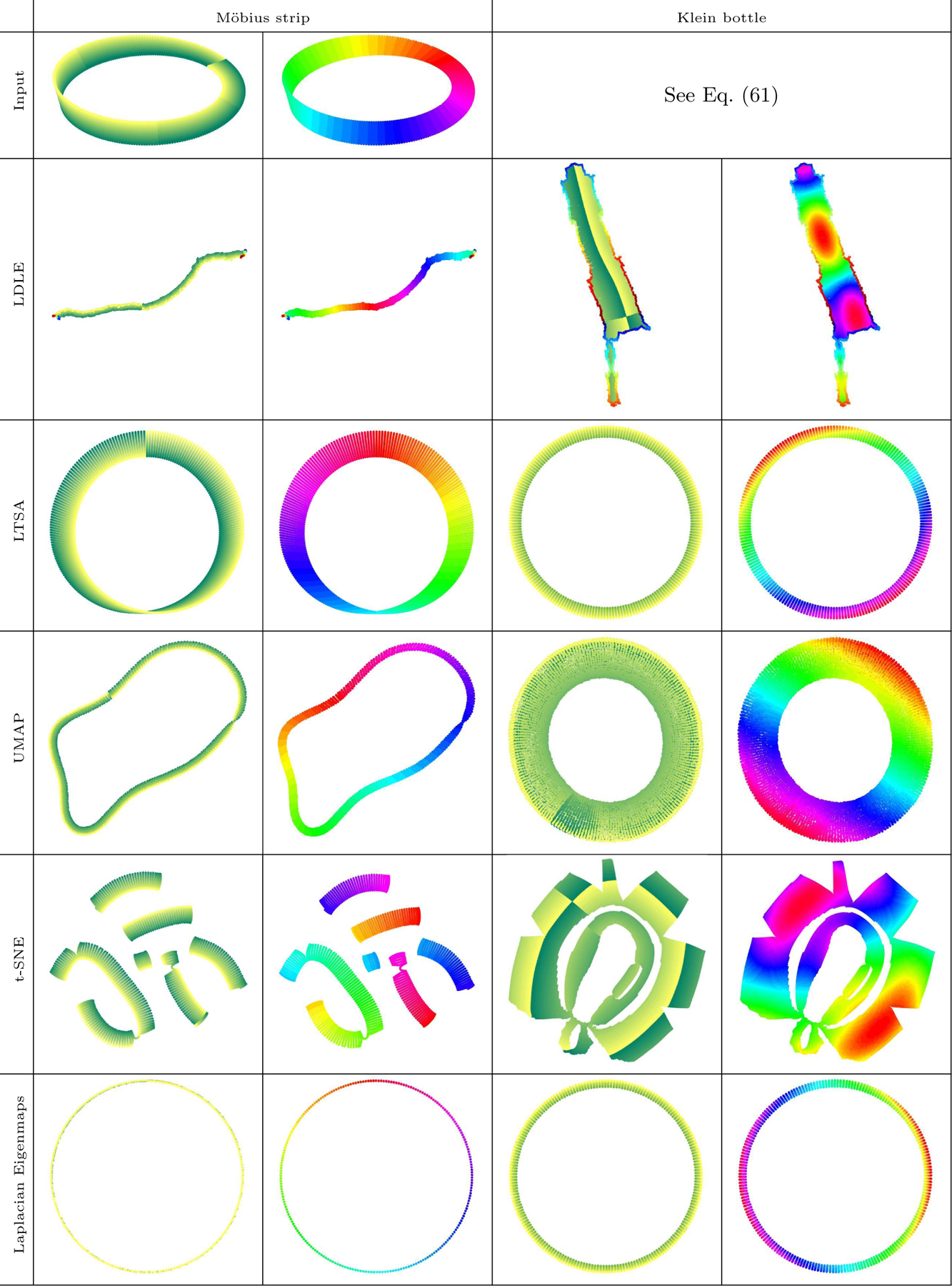
Embeddings of 2d non-orientable manifolds into ${ℝ}^2$. For each manifold, the left and right columns contain the same plots colored by the two parameters of the manifold. A proof of the mathematical correctness of the LDLE embeddings is provided in Figure 31.

An illustration of the global embedding at various stages of Algo. 5 with modified step R2, is provided in Figure 12.

Figure 12:

2d embedding of a sphere at different stages of Algo. 5. For illustration purpose, in the plots in the 2nd and 3rd columns the translation parameter v_m was manually set for those views which do not lie in the set $\mathcal{A}$.

Example. The obtained global embeddings of our square grid with to_tear = True and ν = 3, are shown in Figure 13. Note that the boundary of the obtained embedding is more distorted when the points on the boundary are unknown than when they are known apriori. This is because the intermediate views near the boundary have higher distortion in the former case than in the latter case (see Figure 7).

Figure 13:

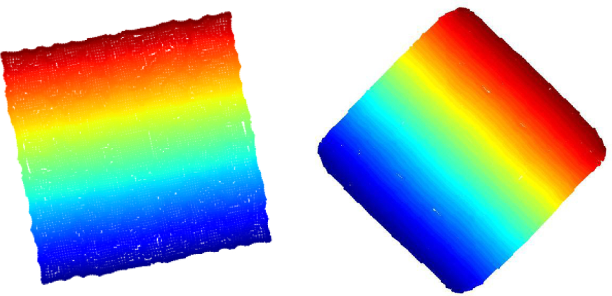
Global embedding of the square grid when the points on the boundary are unknown (left) versus when they are known apriori (right).

5.4. Time Complexity

The worst case time complexity of Algo. 5 is $O\left(N_{r}n{k}_{\text{lv}}^2{d}^2/{\eta }_{\min }\right)$ when to tear is false. It costs an additional time of $\left.O\left(N_r{n}^2\max \left(d,k_{\text{lv}}\log n,n/{\eta }_{\min }^2\right)\right)\right)$ when to tear is true. In practice, one refinement step took about 15 seconds in the above example and between 15–20 seconds for all the examples in Section 6.

6. Experimental Results

We present experiments to compare LDLE² with LTSA (Zhang and Zha, 2003), UMAP (McInnes et al., 2018), t-SNE (Maaten and Hinton, 2008) and Laplacian eigenmaps (Belkin and Niyogi, 2003) on several data sets. First, we compare the embeddings of discretized 2d manifolds embedded in ${ℝ}^2$, ${ℝ}^3$ or ${ℝ}^4$, containing about 10⁴ points. These manifolds are grouped based on the presence of the boundary and their orientability as in Sections 6.2, 6.3 and 6.4. The inputs are shown in the figures themselves except for the flat torus and the Klein bottle, as their 4D parameterizations cannot be plotted. Therefore, we describe their construction below. A quantitative comparison of the algorithms is provided in Section 6.2.1. In Section 6.2.2 we assess the robustness of these algorithms to the noise in the data. In Section 6.2.3 we assess the performance of these algorithms on sparse data. Finally, in Section 6.5 we compare the embeddings of some high dimensional data sets.

Flat Torus. A flat torus is a parallelogram whose opposite sides are identified. In our case, we construct a discrete flat torus using a rectangle with sides 2 and 0.5 and embed it in four dimensions as follows,

$$X\left({\theta }_i,{\varphi }_j\right)=\frac{1}{4\pi }\left(4cos\left({\theta }_i\right),4\sin \left({\theta }_i\right),\cos \left({\varphi }_j\right),\sin \left({\varphi }_j\right)\right)$$ (59)

where θ_i = 0.01iπ, ϕ_j = 0.04jπ, i ∈ {0,...,199} and j ∈ {0,...,49}.

Klein bottle. A Klein bottle is a non-orientable two dimensional manifold without boundary. We construct a discrete Klein bottle using its 4D Möbius tube representation as follows,

$$X\left({\theta }_i,{\varphi }_j\right)=\left(R\left({\varphi }_j\right)\cos {\theta }_i,R\left({\varphi }_j\right)\sin {\theta }_i,r\sin {\varphi }_j\cos \frac{{\theta }_i}{2},r\sin {\varphi }_j\sin \frac{{\theta }_i}{2}\right)$$ (60)

$$R\left({\varphi }_j\right)=R+r\cos {\varphi }_j$$ (61)

where θ_i = iπ/100, ϕ_j = jπ/25, i ∈ {0,...,199} and j ∈ {0,...,49}.

6.1. Hyperparameters

To embed using LDLE, we use the Euclidean metric and the default values of the hyperparameters and their description are provided in Table 1. Only the value of η_min is tuned across all the examples in Sections 6.2, 6.3 and 6.4 (except for Section 6.2.3), and is provided in Appendix G. For high dimensional data sets in Section 6.5, values of the hyperaparameters which differ from the default values are again provided in Appendix G.

For UMAP, LTSA, t-SNE and Laplacian eigenmaps, we use the Euclidean metric and select the hyperparameters by grid search, choosing the values which result in best visualization quality. For LTSA, we search for optimal n neighbors in {5,10,25,50,75,100}. For UMAP, we use 500 epochs and search for optimal n neighbors in {25,50,100,200} and min dist in {0.01,0.1,0.25,0.5}. For t-SNE, we use 1000 iterations and search for optimal perplexity in {30,40,50,60} and early exaggeration in {2,4,6}. For Laplacian eigenmaps, we search for k_nn in {16,25,36,49} and k_tune in {3,7,11}. The chosen values of the hyperparameters are provided in Appendix G. We note that the Laplacian eigenmaps fails to correctly embed most of the examples regardless of the choice of the hyperparameters.

6.2. Manifolds with Boundary

In Figure 14, we show the 2d embeddings of 2d manifolds with boundary, in ${ℝ}^2$ or ${ℝ}^3$, three of which have holes. To a large extent, LDLE preserved the shape of the holes. LTSA perfectly preserved the shape of the holes in the square but deforms it in the Swiss Roll. This is because LTSA embedding does not capture the aspect ratio of the underlying manifold as discussed in Section F. UMAP and Laplacian eigenmaps distorted the shape of the holes and the region around them, while t-SNE produced dissected embeddings. For the sphere with a hole which is a curved 2d manifold with boundary, LTSA, UMAP and Laplacian eigenmaps squeezed it into ${ℝ}^2$ while LDLE and t-SNE tore it apart. The correctness of the LDLE embedding is proved in Figure 31. In the case of noisy swiss roll, LDLE and UMAP produced visually better embeddings in comparison to the other methods.

Figure 14:

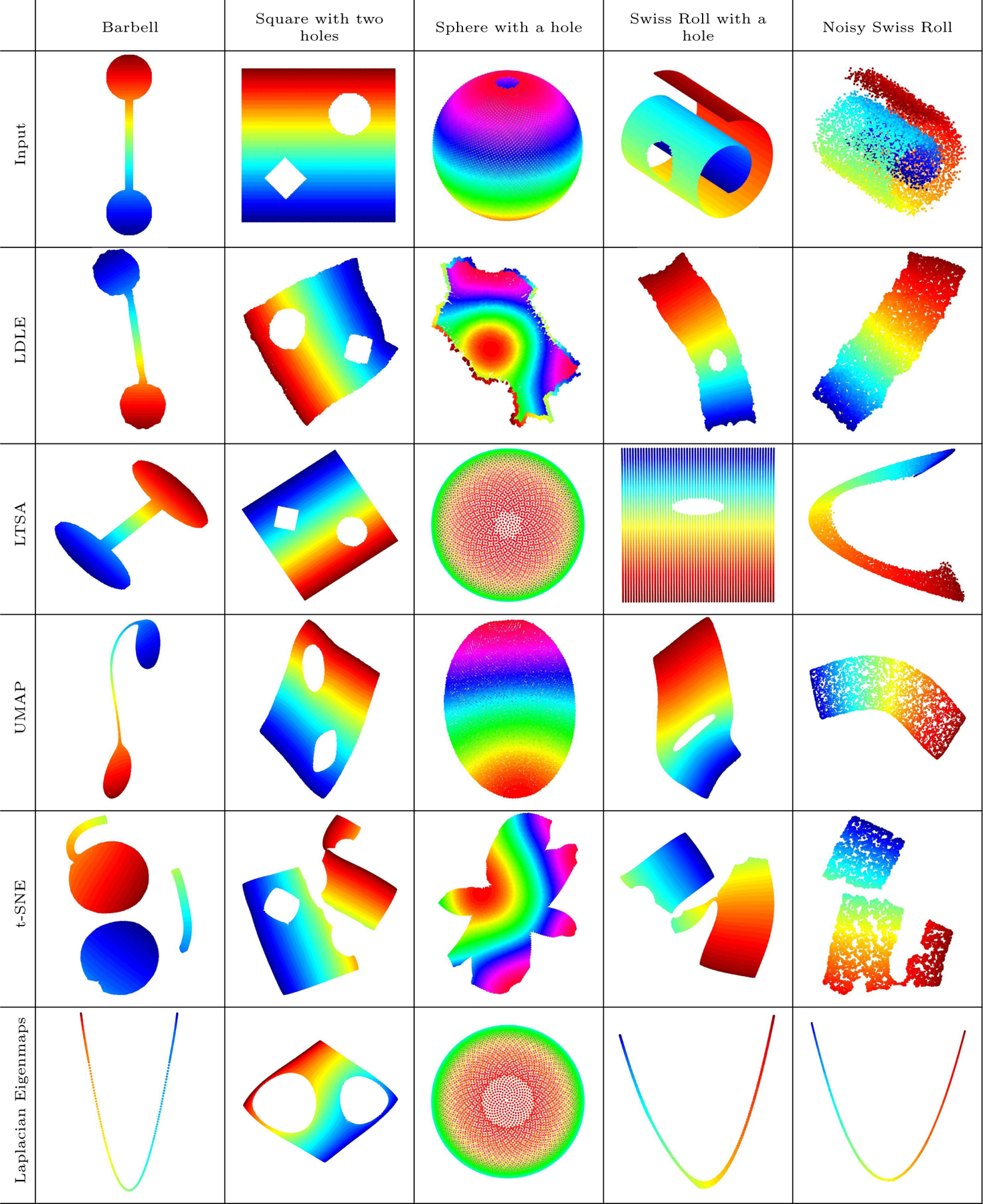
Embeddings of 2d manifolds with boundary into ${ℝ}^2$. The noisy Swiss Roll is constructed by adding uniform noise in all three dimensions, with support on [0,0.05].

We note that the boundaries of the LDLE embeddings in Figure 14 are usually distorted. The cause of this is explained in Remark 4. When the points in the input which lie on the boundary are known apriori then the distortion near the boundary can be reduced using the double manifold as discussed in Remark 5 and shown in Figure 4. The obtained LDLE embeddings when the points on the boundary are known, are shown in Figure 15.

Figure 15:

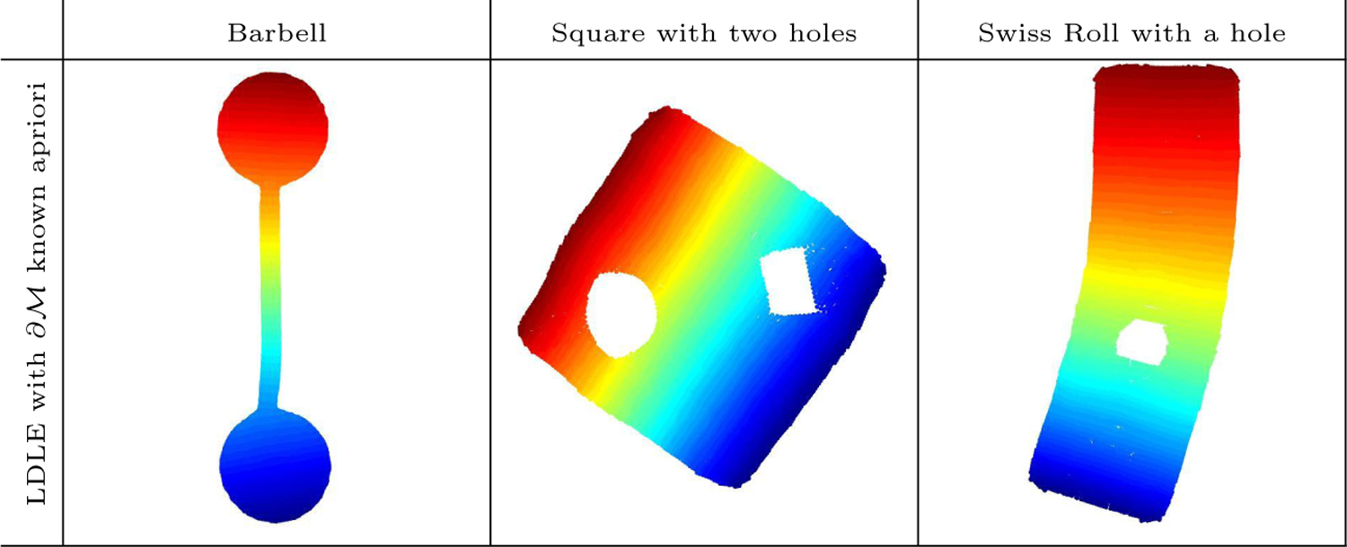
LDLE embeddings when the points on the boundary are known apriori.

6.2.1. Quantitative Comparison

To compare LDLE with other techniques in a quantitative manner, we compute the distortion ${\mathcal{D}}_k$ of the embeddings of the geodesics originating from x_k and then plot the distribution of ${\mathcal{D}}_k$ (see Figure 16). The procedure to compute ${\mathcal{D}}_k$ follows. In the discrete setting, we first define the geodesic between two given points as the shortest path between them which in turn is computed by running Dijkstra algorithm on the graph of 5 nearest neighbors. Here, the distances are measured using the Euclidean metric d_e. Denote the number of nodes on the geodesic between x_k and x_k′ by n_kk′ and the sequence of nodes by ${\left(x_s\right)}_{s=1}^{n_{k{k}^{\prime }}}$ where x₁ = x_k and $x_{n_{k{k}^{\prime }}}=x_{k^{\prime }}$. Denote the embedding of x_k by y_k. Then the length of the geodesic in the latent space between x_k and x_k′, and the length of the embedding of the geodesic between y_k and y_k′ are given by

$$L_{k{k}^{\prime }}={\displaystyle \sum _{s=2}^{n_{k{k}^{\prime }}}{d}_e\left(x_s,x_{s-1}\right)}.$$ (62)

$$L_{k{k}^{\prime }}^g={\displaystyle \sum _{s=2}^{n_{k{k}^{\prime }}}{d}_e\left(y_s,y_{s-1}\right)}.$$ (63)

Finally, the distortion ${\mathcal{D}}_k$ of the embeddings of the geodesics originating from x_k is given by the ratio of maximum expansion and minimum contraction, that is,

$${\mathcal{D}}_k=\underset{k^{\prime }}{\sup }\frac{L_{k{k}^{\prime }}^g}{L_{k{k}^{\prime }}}/\underset{k^{\prime }}{\inf }\frac{L_{k{k}^{\prime }}^g}{L_{k{k}^{\prime }}}=\underset{k^{\prime }}{\sup }\frac{L_{k{k}^{\prime }}^g}{L_{k{k}^{\prime }}}\underset{k^{\prime }}{\sup }\frac{L_{k{k}^{\prime }}}{L_{k{k}^{\prime }}^g}.$$ (64)

Figure 16:

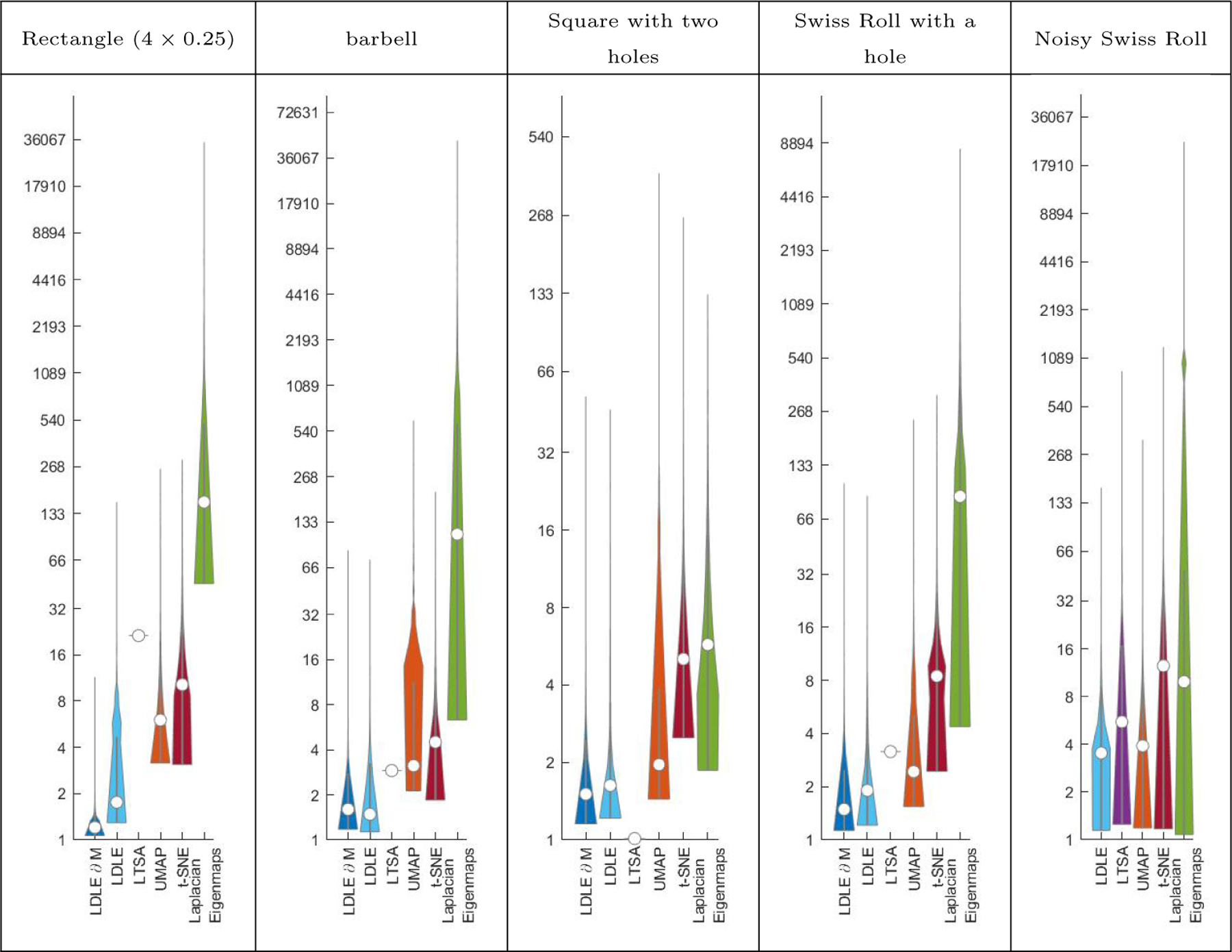
Violin plots (Hintze and Nelson, 1998; Bechtold et al., 2021) for the distribution of ${\mathcal{D}}_k$ (See Eq. (64)). LDLE ∂M means LDLE with boundary known apriori. The white point inside the violin represents the median. The straight line above the end of the violin represents the outliers.

A value of 1 for ${\mathcal{D}}_k$ means the geodesics originating from x_k have the same length in the input and in the embedding space. If ${\mathcal{D}}_k=1$ for all k then the embedding is geometrically, and therefore topologically as well, the same as the input up to scale. Figure 16 shows the distribution of ${\mathcal{D}}_k$ due to LDLE and other algorithms for various examples. Except for the noisy Swiss Roll, LTSA produced the least maximum distortion. Specifically, for the square with two holes, LTSA produced a distortion of 1 suggesting its strength on manifolds with unit aspect ratio. In all other examples, LDLE produced the least distortion except for a few outliers. When the boundary is unknown, the points which result in high ${\mathcal{D}}_k$ are the ones which lie on and near the boundary. When the boundary is known, these are the points which lie on or near the corners (see Figures 4 and 5). We aim to fix this issue in future work.

6.2.2. Robustness to Noise

To further analyze the robustness of LDLE under noise we compare the embeddings of the Swiss Roll with Gaussian noise of increasing variance. The resulting embeddings are shown in Figure 17. Note that certain points on LDLE embeddings have a different colormap than the one used for the input. As explained in Section 5.3, the points which have the same color under this colormap are adjacent on the manifold but away in the embedding. To be precise, these points lie close to the middle of the gap in the Swiss Roll, creating a bridge between those points which would otherwise be far away on a noiseless Swiss Roll. In a sense, these points cause maximum corruption to the geometry of the underlying noiseless manifold. One can say that these points are have adversarial noise, and LDLE embedding can automatically recognize such points. We will further explore this in future work. LTSA, t-SNE and Laplacian Eigenmaps fail to produce correct embeddings while UMAP embeddings also exhibit high quality.

Figure 17:

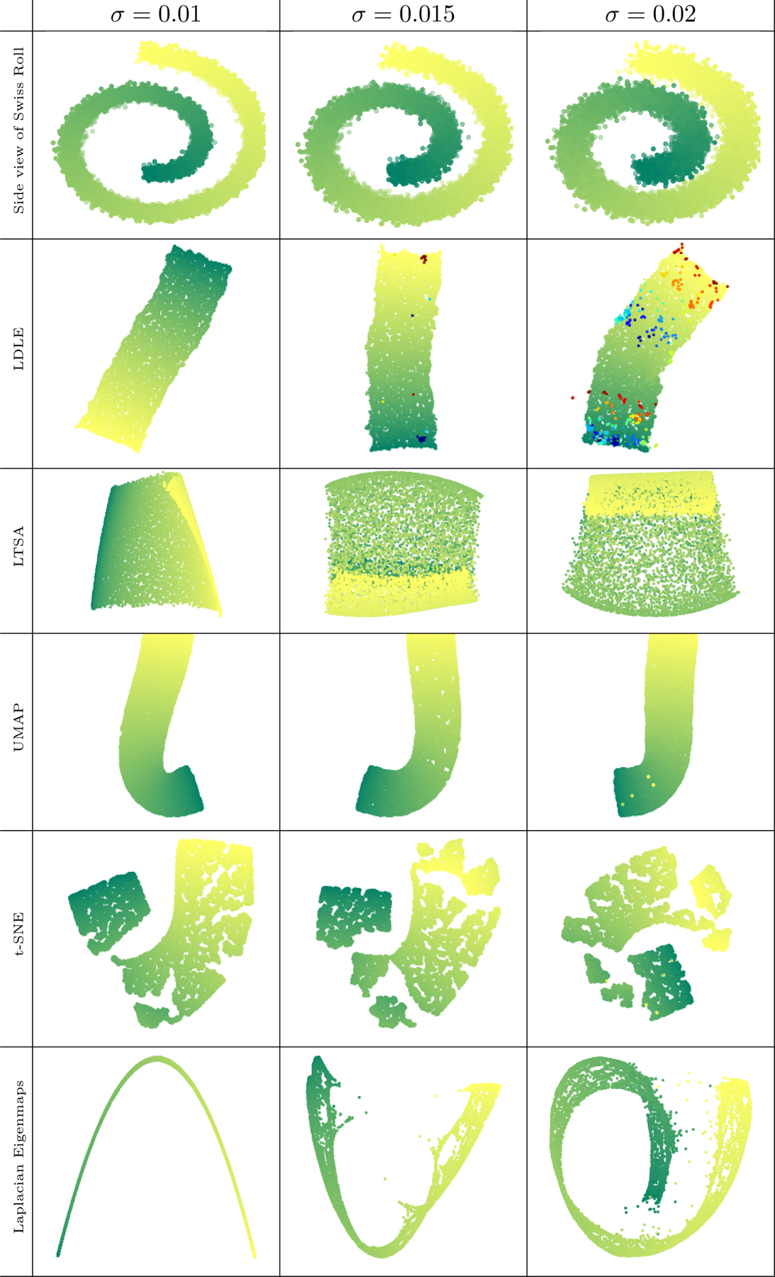
Embeddings of the Swiss Roll with additive noise sampled from the Gaussian distribution of zero mean and a variance of σ² (see Section 6.2.2 for details).

6.2.3. Sparsity

A comparison of the embeddings of the Swiss Roll with decreasing resolution and increasing sparsity is provided in Figure 18. Unlike LTSA and Laplacian Eigenmaps, the embeddings produced by LDLE, UMAP and t-SNE are of high quality. Note that when the resolution is 10, LDLE embedding of some points have a different colormap. Due to sparsity, certain points on the opposite sides of the gap between the Swiss Roll are neighbors in the ambient space as shown in Figure 32 in Appendix H. LDLE automatically tore apart these erroneous connections and marked them at the output using a different colormap. A discussion on sample size requirement for LDLE follows.

Figure 18:

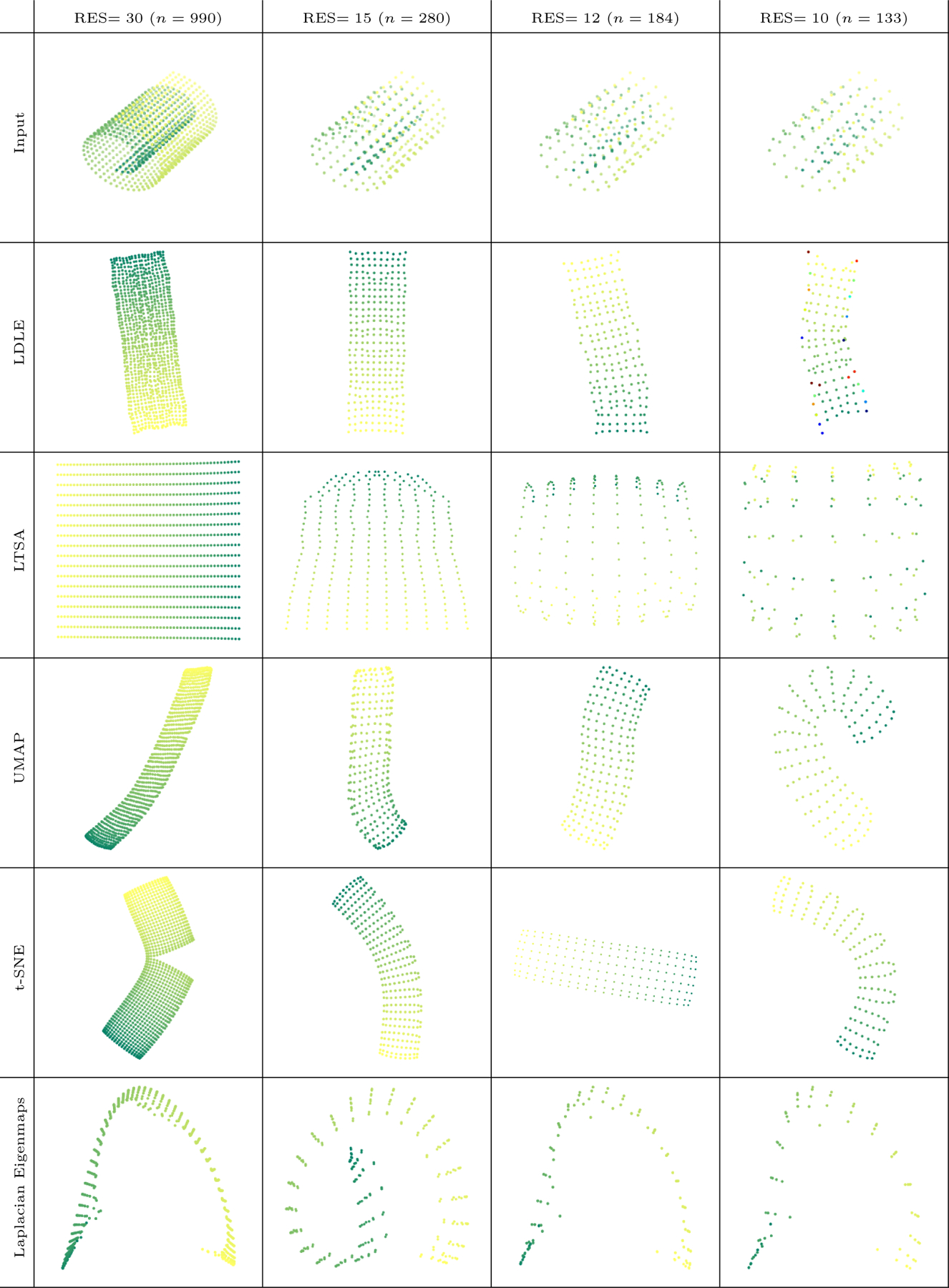
Embeddings of the Swiss Roll with decreasing resolution and increasing sparsity (see Section 6.2.3 for details). Note that when RES= 7 (n = 70) none of the above method produced a correct embedding.

The distortion of LDLE embeddings directly depend on the distortion of the constructed local parameterizations, which in turn depends on reliable estimates of the graph Laplacian and its eigenvectors. The work in (Belkin and Niyogi, 2008; Hein et al., 2007; Trillos et al., 2020; Cheng and Wu, 2021) provided conditions on the sample size and the hyperparameters such as the kernel bandwidth, under which the graph Laplacian and its eigenvectors would converge to their continuous counterparts. A similar analysis in the setting of self-tuned kernels used in our approach (see Algo. 1) is also provided in (Cheng and Wu, 2020). These imply that, for a faithful estimation of graph Laplacian and its eigenvectors, the hyperparameter k_tune (see Table 1) should be small enough so that the local scaling factors σ_k (see Algo. 1) are also small, while the size of the data n should be large enough so that $n{\sigma }_k^{d+2}/\log \left(n\right)$ is sufficiently large for all k ∈ {1,...,n}. This suggests that n needs to be exponential in d and inversely related to σ_k. However, in practice, the data is usually given and therefore n is fixed. So the above mainly states that to obtain accurate estimates, the hyperparameter k_tune must be decreased. This indeed holds as we had to decrease k_tune from 7 to 2 (see Appendix G) to produce LDLE embeddings of high quality for increasingly sparse Swiss Roll in Figure 18.

6.3. Closed Manifolds

In Figure 19, we show the 2d embeddings of 2d manifolds without a boundary, a curved torus in ${ℝ}^3$ and a flat torus in ${ℝ}^4$. LDLE produced similar representation for both the inputs. None of the other methods do that. The main difference in the LDLE embedding of the two inputs is based on the boundary of the embedding. It is composed of many small line segments for the flat torus, and many small curved segments for the curved torus. This is clearly because of the difference in the curvature of the two inputs, zero everywhere for the flat torus and non-zero almost everywhere on the curved torus. The mathematical correctness of the LDLE embeddings using the cut and paste argument is shown in Figure 31. LTSA, UMAP and Laplacian eignemaps squeezed both the manifolds into ${ℝ}^2$ while the t-SNE embedding is non-interpretable.

6.4. Non-Orientable Manifolds

In Figure 20, we show the 2d embeddings of non-orientatble 2d manifolds, a Möbius strip in ${ℝ}^3$ and a Klein bottle in ${ℝ}^4$. Laplacian eigenmaps produced incorrect embeddings, t-SNE produced dissected and non-interpretable embeddings and LTSA and UMAP squeezed the inputs into ${ℝ}^2$. LDLE produced mathematically correct embeddings by tearing apart both inputs to embed them into ${ℝ}^2$ (see Figure 31).

6.5. High Dimensional Data

6.5.1. Synthetic Sensor Data

In Figure 21, motivated from (Peterfreund et al., 2020), we embed a 42 dimensional synthetic data set representing the signal strength of 42 transmitters at about n = 6000 receiving locations on a toy floor plan. The transmitters and the receivers are distributed uniformly across the floor. Let ${\left(t_{r_k}\right)}_{k=1}^{42}$ be the transmitter locations and r_i be the ith receiver location. Then the ith data point x_i is given by ${\left(e^{-{‖r_i-t_{r_k}‖}_2^2}\right)}_{k=1}^{42}$. The resulting data set is embedded using and other algorithms into ${ℝ}^2$. The hyperparameters resulting in the most visually appealing embeddings were identified for each algorithm and are provided in Table 2. The obtained embeddings are shown in Figure 21. The shapes of the holes are best preserved by LTSA, then LDLE followed by the other algorithms. The corners of the LDLE embedding are more distorted. The reason for distorted corners is given in Remark 4.

Figure 21:

Embedding of the synthetic sensor data into ${ℝ}^2$ (see Section 6.5 for details).

6.5.2. Face Image Data

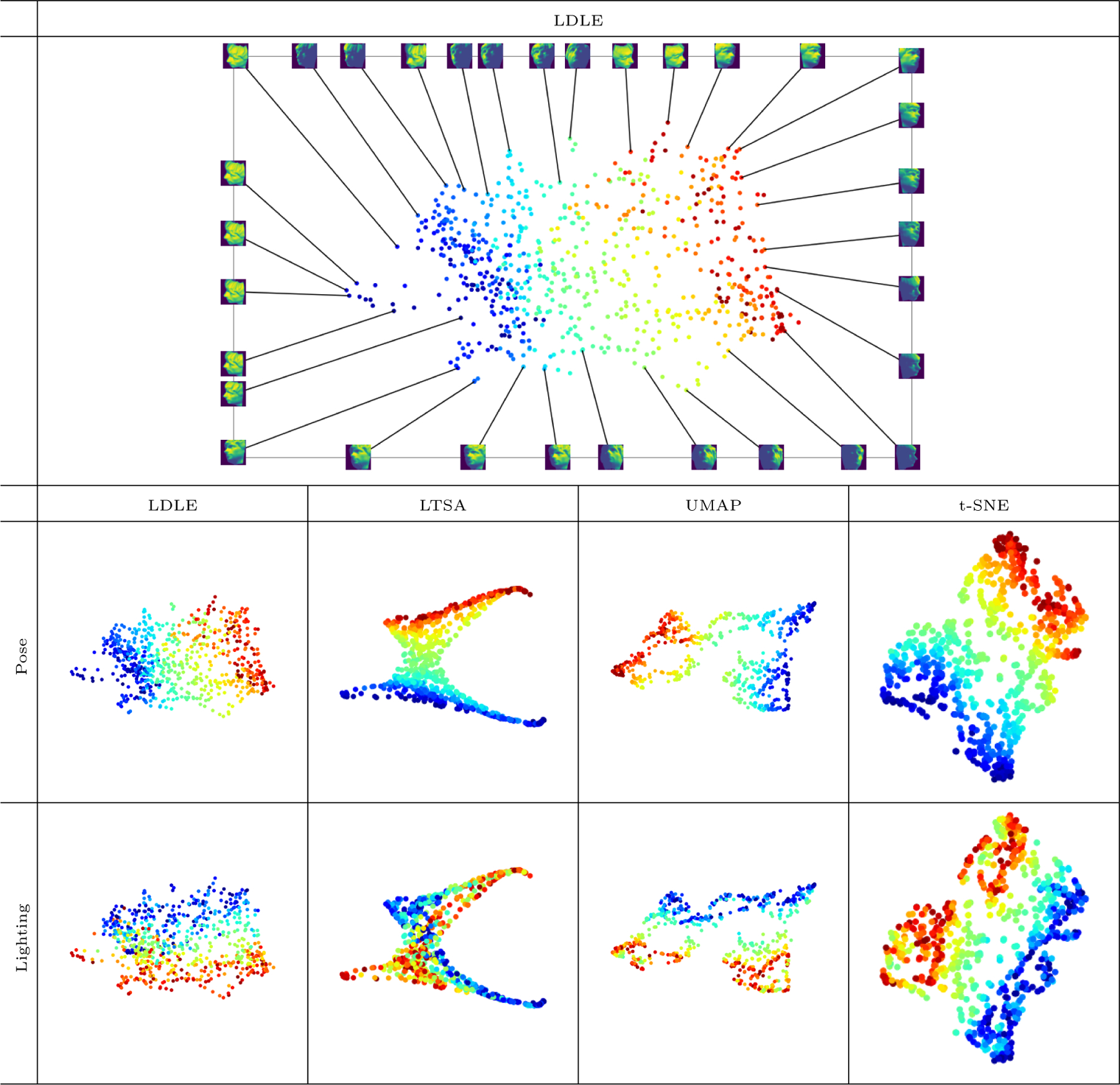
In Figure 22, we show the embedding obtained by applying LDLE on the face image data (Tenenbaum et al., 2000) which consists of a sequence of 698 64-by-64 pixel images of a face rendered under various pose and lighting conditions. These images are converted to 4096 dimensional vectors, then projected to 100 dimensions through PCA while retaining about 98% of the variance. These are then embedded using LDLE and other algorithms into ${ℝ}^2$. The hyperparameters resulting in the most visually appealing embeddings were identified for each algorithm and are provided in Table 5. The resulting embeddings are shown in Figure 23 colored by the pose and lighting of the face. Note that values of the pose and lighting variables for all the images are provided in the data set itself. We have displayed face images corresponding to few points of the LDLE embeddings as well. Embeddings due to all the techniques except LTSA reasonably capture both the pose and lighting conditions.

Figure 22:

Embedding of the face image data set (Tenenbaum et al., 2000) into ${ℝ}^2$ colored by the pose and lighting conditions (see Section 6.5 for details).

Figure 23:

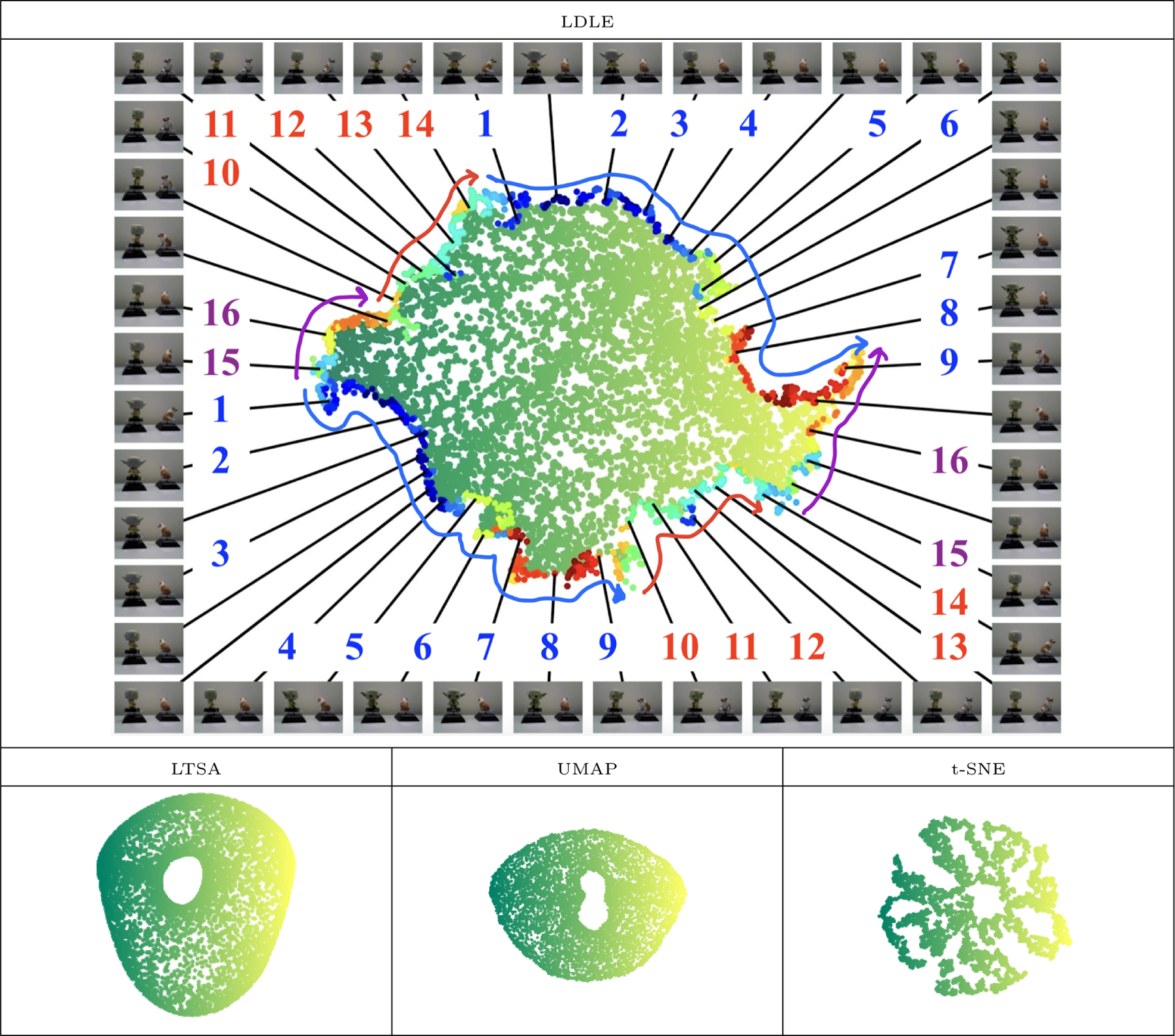
Embeddings of snapshots of a platform with two objects, Yoda and a bull dog, each rotating at a different frequency, such that the underlying topology is a torus (see Section 6.5 for details).

6.5.3. Rotating Yoda-Bulldog Data Set

In Figure 23, we show the 2d embeddings of the rotating figures data set presented in (Lederman and Talmon, 2018). It consists of 8100 snapshots taken by a camera of a platform with two objects, Yoda and a bull dog, rotating at different frequencies. Therefore, the underlying 2d parameterization of the data should render a torus. The original images have a dimension of 320 × 240 × 3. In our experiment, we first resize the images to half the original size and then project them to 100 dimensions through PCA (Jolliffe and Cadima, 2016) while retaining about 98% variance. These are then embedded using LDLE and other algorithms into ${ℝ}^2$. The hyperparameters resulting in the most visually appealing embeddings were identified for each algorithm and are provided in Table 5. The resulting embeddings are shown in Figure 23 colored by the first dimension of the embedding itself. LTSA and UMAP resulted in a squeezed torus. LDLE tore apart the underlying torus and automatically colored the boundary of the embedding to suggest the gluing instructions. By tracing the color on the boundary we have manually drawn the arrows. Putting these arrows on a piece of paper and using cut and past argument one can establish that the embedding represents a torus (see Figure 31). The images corresponding to a few points on the boundary are shown. Pairs of images with the same labels represent the two sides of the curve along which LDLE tore apart the torus, and as is evident these pairs are similar.

7. Conclusion and Future Work

We have presented a new bottom-up approach (LDLE) for manifold learning which constructs low-dimensional low distortion local views of the data using the low frequency global eigenvectors of the graph Laplacian, and registers them to obtain a global embedding. Through various examples we demonstrated that LDLE competes with the other methods in terms of visualization quality. In particular, the embeddings produced by LDLE preserved distances upto a constant scale better than those produced by UMAP, t-SNE, Laplacian Eigenmaps and for the most part LTSA too. We also demonstrated that LDLE is robust to the noise in the data and produces fine embeddings even when the data is sparse. We also showed that LDLE can embed closed as well as non-orientable manifolds into their intrinsic dimension, a feature that is missing from the existing techniques. Some of the future directions of our work are as follows.

It is only natural to expect real world data sets to have boundary and to have many corners. As observed in the experimental results, when the boundary of the manifold is unknown, then the LDLE embedding tends to have distorted boundary. Even when the boundary is known, the embedding has distorted corners. This is caused by high distortion views near the boundary (see Figures 4 and 5). We aim to fix this issue in our future work. One possible resolution could be based on (Berry and Sauer, 2017) which presented a method to approximately calculate the distance of the points from the boundary.

When the data represents a mixture of manifolds, for example, a pair of possibly intersecting spheres or even manifolds of different intrinsic dimensions, it is also natural to expect a manifold learning technique to recover a separate parameterization for each manifold and provide gluing instructions at the output. One way is to perform manifold factorization (Zhang et al., 2021) or multi-manifold clustering (Trillos et al., 2021) on the data to recover sets of points representing individual manifolds and then use manifold learning on these separately. We aim to adapt LDLE to achieve this.

The spectrum of the Laplacian has been used in prior work for anomaly detection (Cloninger and Czaja, 2015; Mishne and Cohen, 2013; Cheng et al., 2018; Cheng and Mishne, 2020; Mishne et al., 2019). Similar to our approach of using a subset of Laplacian eigenvectors to construct low distortion local views in lower dimension, in (Mishne et al., 2018; Cheng and Mishne, 2020), subsets of Laplacian eigenvectors were identified so as to separate small clusters from a large background component. As shown in Figures 4 and 5, LDLE produced high distortion local views near the boundary and the corners, though these are not outliers. However, if we consider a sphere with outliers (say, a sphere with noise only at the north pole as in Figure 24), then the distortion of the local views containing the outliers is higher than the rest of the views. Therefore, the distortion of the local views can help find anomalies in the data. We aim to further investigate this direction to develop an anomaly detection technique.

Figure 24:

Local views containing outliers exhibit high distortion. (left) Input data ${\left(x_k\right)}_{k=1}^n$. (middle) x_k colored by the distortion ζ_kk of Φ_k on U_k. (right) y_k colored by ζ_kk.

Similar to the approach of denoising a signal by retaining low frequency components, our approach uses low frequency Laplacian eigenvectors to estimate local views. These eigenvectors implicitly capture the global structure of the manifold. Therefore, to construct local views, unlike LTSA which directly relies on the local configuration of data which may be noisy, LDLE relies on the local elements of low frequency global eigenvectors of the Laplacian which are supposed to be robust to the noise. Practical implication of this is shown in Figure 17 to some extent while we aim to further investigate the theoretical implications.

A. First Proof of Theorem 2

Choose ϵ > 0 so that the exponential map ${\exp }_x:T_x\mathcal{M}\to \mathcal{M}$ is a well defined diffeomorphism on ${\mathcal{B}}_{2ϵ}\subset T_x\mathcal{M}$ where $T_x\mathcal{M}$ is the tangent space to $\mathcal{M}$ at x, exp_x(0) = x and

$${\mathcal{B}}_{ϵ}=\left\{v\in T_x\mathcal{M}|{‖v‖}_2<ϵ\right\}.$$ (65)

Then using (Canzani, 2013, lem. 48, prop. 50, th. 51), for all $y\in B_{ϵ}\left(x\right)$ such that

$$B_{ϵ}\left(x\right)=\left\{y\in \mathcal{M}|d_g\left(x,y\right)<ϵ\right\}$$ (66)

we have,

$$p\left(t,x,y\right)=G\left(t,x,y\right)\left(u_0\left(x,y\right)+t{u}_1\left(x,y\right)+O\left(t^2\right)\right),$$ (67)

where

$$G\left(t,x,y\right)=\frac{e^{-d_g{\left(x,y\right)}^2/4t}}{{\left(4\pi t\right)}^{d/2}},$$ (68)

$$u_0\left(x,y\right)=1+O\left({‖v‖}^2\right),\hspace{0.33em}\hspace{0.17em}y={\exp }_x\left(v\right),\hspace{0.33em}v\in T_x\mathcal{M},$$ (69)

and for $f\in C\left(\mathcal{M}\right)$, the following hold

$$f\left(x\right)=\underset{t\to 0}{\lim }{\displaystyle {\int }_{M}p\left(t,x,y\right)f\left(y\right){\omega }_g\left(y\right)}$$ (70)

$$=\underset{t\to 0}{\lim }{\displaystyle {\int }_{B_{ϵ}\left(x\right)}p\left(t,x,y\right)f\left(y\right){\omega }_g\left(y\right)},$$ (71)

$$f\left(x\right)=\underset{t\to 0}{\lim }{\displaystyle {\int }_{B_{ϵ}\left(x\right)}G\left(t,x,y\right)f\left(y\right){\omega }_g\left(y\right)},$$ (72)

$$u_1\left(x,x\right)f\left(x\right)=\underset{t\to 0}{\lim }{\displaystyle {\int }_{B_{ϵ}\left(x\right)}G\left(t,x,y\right)u_1\left(x,y\right)f\left(y\right){\omega }_g\left(y\right)}.$$ (73)

Using the above equations and the definition of Ψ_kij(y) in Eq. (15) and A_kij in Eq. (16) we compute the limiting value of the scaled local correlation (see Eq. (19)),

$${\tilde{A}}_{kij}=\underset{t\to 0}{\lim }\frac{A_{kij}}{2t}$$ (74)

$$=\underset{t\to 0}{\lim }\frac{1}{2t}{\displaystyle {\int }_{M}p\left(t,x_k,y\right){\mathrm{\Psi }}_{kij}\left(y\right){\omega }_g\left(y\right)}.$$ (75)

which will turn out to be the inner product between the gradients of the eigenfunctions ϕ_i and ϕ_j at x_k. We start by choosing an ϵ_k > 0 so that ${\exp }_{x_k}$ is a well defined diffeomorphism on ${\mathcal{B}}_{2{ϵ}_k}\subset T_{x_k}\mathcal{M}$. Using Eq. (71) we change the region of integration from $\mathcal{M}$ to $B_{{ϵ}_k}\left(x_k\right)$,

$${\tilde{A}}_{kij}=\underset{t_k\to 0}{\lim }\frac{1}{2t_k}{\displaystyle {\int }_{B_{{ϵ}_k}\left(x_k\right)}p\left(t_k,x_k,y\right){\mathrm{\Psi }}_{kij}\left(y\right){\omega }_g\left(y\right)}.$$ (76)

Substitute p(t_k,x_k,y) from Eq. (67) and simplify using Eq. (72, 73) and the fact that Ψ_kij(x_k) = 0 to get

$$\begin{array}{l}{\tilde{A}}_{kij}=\underset{t_k\to 0}{\lim }\frac{1}{2t_k}{\displaystyle {\int }_{B_{{ϵ}_k}\left(x_k\right)}G\left(t_k,x_k,y\right)\left(u_0\left(x_k,y\right)+t_k{u}_1\left(x_k,y\right)+O\left(t_k^2\right)\right){\mathrm{\Psi }}_{kij}\left(y\right){\omega }_g\left(y\right)}.\\ \hspace{1em}\hspace{0.17em}\hspace{0.17em}\hspace{0.17em}=\underset{t_k\to 0}{\lim }\left(\frac{1}{2t_k}{\displaystyle {\int }_{B_{{ϵ}_k}\left(x_k\right)}G\left(t_k,x_k,y\right)u_0\left(x_k,y\right){\mathrm{\Psi }}_{kij}\left(y\right){\omega }_g\left(y\right)+}\right.\\ \hspace{1em}\hspace{1em}\hspace{1em}\hspace{1em}\hspace{1em}\hspace{1em}\hspace{1em}\hspace{1em}\hspace{1em}\hspace{1em}\hspace{1em}\hspace{1em}\hspace{0.17em}\hspace{0.17em}\hspace{0.17em} \left.\frac{t_k{u}_1\left(x_k,x_k\right){\mathrm{\Psi }}_{kij}\left(x_k\right)+O\left(t_k^2\right){\mathrm{\Psi }}_{kij}\left(x_k\right)}{2t_k}\right)\\ \hspace{1em}\hspace{0.17em}\hspace{0.17em}\hspace{0.17em}=\underset{t_k\to 0}{\lim }\frac{1}{2t_k}{\displaystyle {\int }_{B_{{ϵ}_k}\left(x_k\right)}G\left(t_k,x_k,y\right)u_0\left(x_k,y\right){\mathrm{\Psi }}_{kij}\left(y\right){\omega }_g\left(y\right)}.\end{array}$$ (77)

Replace $y\in B_{{ϵ}_k}\left(x_k\right)$ by ${\exp }_{x_k}\left(v\right)$ where $v\in {\mathcal{B}}_{{ϵ}_k}\subset T_{x_k}\mathcal{M}$ and $‖v‖=d_g\left(x_k,y\right)$. Denote the Jacobian for the change of variable by J(v) i.e.$J\left(v\right)=\frac{d}{dv}{\exp }_{x_k}\left(v\right)$. Note that ${\exp }_{x_k}\left(0\right)=x_k$ and J(0) = I. Using the Taylor expansion of ϕ_i and ϕ_j about 0 we obtain

$$\begin{array}{l}{\varphi }_s\left(y\right)={\varphi }_s\left({\exp }_{x_k}\left(v\right)\right)={\varphi }_s\left({\exp }_{x_k}\left(0\right)\right)+\nabla {\varphi }_s{\left({\exp }_{x_k}\left(0\right)\right)}^{T}J\left(0\right)v+O\left({‖v‖}^2\right)\\ \hspace{1em}\hspace{1em}\hspace{0.17em}\hspace{0.17em}\hspace{0.17em}\hspace{0.17em}\hspace{0.17em}\hspace{0.17em}\hspace{0.17em}\hspace{0.17em}\hspace{0.17em}\hspace{0.17em}\hspace{0.17em}\hspace{0.17em}\hspace{0.17em}\hspace{0.17em}\hspace{0.17em}\hspace{0.17em}\hspace{0.17em}\hspace{0.17em}\hspace{0.17em}\hspace{0.17em}\hspace{0.17em}\hspace{0.17em}\hspace{0.17em}\hspace{0.17em}\hspace{0.17em}\hspace{0.17em}\hspace{0.17em}\hspace{0.17em}\hspace{0.17em}\hspace{0.17em}\hspace{0.17em}\hspace{0.17em}\hspace{0.17em}\hspace{0.17em}={\varphi }_s\left(x_k\right)+\nabla {\varphi }_s{\left(x_k\right)}^{T}v+O\left({‖v‖}^2\right),\hspace{0.33em}\hspace{0.17em}s=i,j.\end{array}$$ (78)

Substituting the above equation in the definition of Ψ_kij(y) (see Eq. (15)) we get

$$\begin{array}{l}{\mathrm{\Psi }}_{kij}\left(y\right)={\mathrm{\Psi }}_{kij}\left({\exp }_{x_k}\left(v\right)\right)\\ \hspace{0.17em}\hspace{0.17em}\hspace{0.17em}\hspace{0.17em}\hspace{0.17em}\hspace{0.17em}\hspace{0.17em}\hspace{0.17em}\hspace{0.17em}\hspace{0.17em}\hspace{0.17em}\hspace{0.17em}\hspace{0.17em}\hspace{0.17em}\hspace{0.17em} =v^T\nabla {\varphi }_i\nabla {\varphi }_j^{T}v+\left(\nabla {\varphi }_i^{T}v+\nabla {\varphi }_j^{T}v\right)O\left({‖v‖}^2\right)+O\left({‖v‖}^4\right),\end{array}$$ (79)

where ∇ϕ_s ≡ ∇ϕ_s(x_k),s = i,j. Now we substitute Eq. (79, 68, 69) in Eq. (77) while replacing variable y with ${\exp }_{x_k}\left(v\right)$ where J(v) is the Jacobian for the change of variable as before, to get

$$\begin{array}{l}{\tilde{A}}_{kij}=\underset{t_k\to 0}{\lim }\frac{1}{2t_k}{\displaystyle {\int }_{{\mathcal{B}}_{{ϵ}_k}}\frac{e^{-{‖v‖}^2/4t_k}}{{\left(4\pi t_k\right)}^{d/2}}\left(1+O\left({‖v‖}^2\right)\right){\mathrm{\Psi }}_{kij}\left({\exp }_{x_k}\left(v\right)\right)J\left(v\right)dv}\\ \hspace{0.17em}\hspace{0.17em}\hspace{0.17em}\hspace{0.17em}\hspace{0.17em}\hspace{0.17em}\hspace{0.17em}\hspace{0.17em} =L_1+L_2,\end{array}$$ (80)

where L₁ and L₂ are the terms obtained by expanding 1 + O(‖v‖²) in the integrand. We will show that L₂ = 0 and ${\tilde{A}}_{kij}=L_1=\nabla {\varphi }_i^T\nabla {\varphi }_j$.

$$\begin{array}{l}{L}_2=\underset{t_k\to 0}{\lim }\frac{1}{2t_k}{\displaystyle {\int }_{{\mathcal{B}}_{{ϵ}_k}}\frac{e^{-{‖v‖}^2/4t_k}}{{\left(4\pi t_k\right)}^{d/2}}O\left({‖v‖}^2\right)\left(\text{tr}\left(\nabla {\varphi }_i\nabla {\varphi }_j^{T}v{v}^T\right)+\right.}\\ \hspace{0.17em}\hspace{0.17em}\hspace{0.17em}\hspace{0.17em}\hspace{0.17em}\hspace{0.17em}\hspace{0.17em}\hspace{0.17em}\hspace{0.17em}\hspace{0.17em}\hspace{0.17em}\hspace{0.17em}\hspace{0.17em}\hspace{0.17em}\hspace{0.17em}\hspace{0.17em}\hspace{0.17em}\hspace{0.17em}\hspace{0.17em}\hspace{0.17em}\hspace{0.17em}\hspace{0.17em}\hspace{0.17em}\hspace{0.17em}\hspace{0.17em}\hspace{0.17em}\hspace{0.17em}\hspace{0.17em}\hspace{0.17em}\hspace{0.17em}\hspace{0.17em}\hspace{0.17em}\hspace{0.17em}\hspace{0.17em}\hspace{0.17em}\hspace{0.17em}\hspace{0.17em}\hspace{0.17em}\hspace{1em}\hspace{1em}\hspace{1em}\left.\left(\nabla {\varphi }_i^{T}v+\nabla {\varphi }_j^{T}v\right)O\left({‖v‖}^2\right)+O\left({‖v‖}^4\right)\right)J\left(v\right)dv\\ \hspace{0.17em}\hspace{0.17em}\hspace{0.17em}\hspace{0.17em}\hspace{0.17em}=\underset{t_k\to 0}{\lim }\frac{1}{2t_k}\left(O\left(t_k^2\right)+0+0+O\left(t_k^4\right)\right)\\ \hspace{0.17em}\hspace{0.17em}\hspace{0.17em}\hspace{0.17em}\hspace{0.17em}=0.\end{array}$$ (81)

Therefore,

$$\begin{gathered} {\tilde{A}}_{kij}=L_1 \\ \hspace{0.17em}\hspace{0.17em}\hspace{0.17em}\hspace{0.17em}\hspace{0.17em}\hspace{0.17em}\hspace{0.17em}\hspace{0.17em} =\underset{t_k\to 0}{\lim }\frac{1}{2t_k}{\displaystyle {\int }_{{\mathcal{B}}_{{ϵ}_k}}\frac{e^{-{‖v‖}^2/4t_k}}{{\left(4\pi t_k\right)}^{d/2}}{\mathrm{\Psi }}_{kij}\left({\exp }_{x_k}\left(v\right)\right)J\left(v\right)dv} \end{gathered}$$ (82)

$$\begin{array}{l} =\underset{t_k\to 0}{\lim }\frac{1}{2t_k}{\displaystyle {\int }_{{\mathcal{B}}_{{ϵ}_k}}\frac{e^{-{‖v‖}^2/4t_k}}{{\left(4\pi t_k\right)}^{d/2}}\left(v^T\nabla {\varphi }_i\nabla {\varphi }_j^{T}v+\right.}\\ \hspace{0.17em}\hspace{0.17em}\hspace{0.17em}\hspace{0.17em}\hspace{0.17em}\hspace{0.17em}\hspace{0.17em}\hspace{0.17em}\hspace{0.17em}\hspace{0.17em}\hspace{0.17em}\hspace{0.17em}\hspace{0.17em}\hspace{0.17em}\hspace{0.17em}\hspace{0.17em}\hspace{0.17em}\hspace{0.17em}\hspace{0.17em}\hspace{0.17em}\hspace{0.17em}\hspace{0.17em}\hspace{0.17em}\hspace{0.17em}\hspace{0.17em}\hspace{0.17em}\hspace{0.17em}\hspace{0.17em}\hspace{0.17em}\hspace{0.17em}\left.\left(\nabla {\varphi }_i^{T}v+\nabla {\varphi }_j^{T}v\right)O\left({‖v‖}^2\right)+O\left({‖v‖}^4\right)\right)J\left(v\right)dv\\ =\underset{t_k\to 0}{\lim }\frac{1}{2t_k}{\displaystyle {\int }_{{\mathcal{B}}_{{ϵ}_k}}\frac{e^{-{‖v‖}^2/4t_k}}{{\left(4\pi t_k\right)}^{d/2}}{v}^T\nabla {\varphi }_i\nabla {\varphi }_j^{T}vJ\left(v\right)dv+\frac{0+0+O\left(t_k^2\right)}{2t_k}}\\ =\underset{t_k\to 0}{\lim }\frac{1}{2t_k}{\displaystyle {\int }_{{\mathcal{B}}_{{ϵ}_k}}\frac{e^{-{‖v‖}^2/4t_k}}{{\left(4\pi t_k\right)}^{d/2}}{v}^T\nabla {\varphi }_i\nabla {\varphi }_j^{T}vJ\left(v\right)dv.}\end{array}$$ (83)

Substitution of t_k = 0 leads to the indeterminate form $\frac{0}{0}$. Therefore, we apply L’Hospital’s rule and then Leibniz integral rule to get,

$$\begin{array}{l}{\tilde{A}}_{kij}=\underset{t_k\to 0}{\lim }\frac{1}{2}{\displaystyle {\int }_{{\mathcal{B}}_{{ϵ}_k}}\left(\frac{{‖v‖}^2}{4t_k^2}-\frac{d}{2t_k}\right)\frac{e^{-{‖v‖}^2/4t_k}}{{\left(4\pi t_k\right)}^{d/2}}{v}^T\nabla {\varphi }_i\nabla {\varphi }_j^{T}vJ\left(v\right)dv}\\ \hspace{1em}\hspace{0.17em}\hspace{0.17em}\hspace{0.17em}=\text{tr}\left(\frac{1}{2}\nabla {\varphi }_i\nabla {\varphi }_j^T\underset{t_k\to 0}{\lim }{\displaystyle {\int }_{{\mathcal{B}}_{{ϵ}_k}}\left(\frac{{‖v‖}^2}{4t_k^2}-\frac{d}{2t_k}\right)\frac{e^{-{‖v‖}^2/4t_k}}{{\left(4\pi t_k\right)}^{d/2}}v{v}^{T}J\left(v\right)dv}\right)\\ \hspace{1em}\hspace{0.17em}\hspace{0.17em}\hspace{0.17em}=\text{tr}\left(\frac{1}{2}\nabla {\varphi }_i\nabla {\varphi }_j^T\left(\underset{t_k\to 0}{\lim }\left(\frac{\left(12+4\left(d-1\right)\right)t_k^2}{4t_k^2}-\frac{2t_{k}d}{2t_k}\right)I+O\left(t_k\right)I\right)\right)\\ \hspace{1em}\hspace{0.17em}\hspace{0.17em}\hspace{0.17em}=\nabla {\varphi }_i^T\nabla {\varphi }_j.\end{array}$$ (84)

Finally, note that the Eq. (82) is same as the following equation with y replaced by ${\exp }_{x_k}\left(v\right)$,

$${\tilde{A}}_{kij}=\underset{t_k\to 0}{\lim }\frac{1}{2t_k}{\displaystyle {\int }_{B_{{ϵ}_k}\left(x_k\right)}G\left(t_k,x_k,y\right){\mathrm{\Psi }}_{kij}\left(y\right){\omega }_g\left(y\right)}.$$ (85)

We used the above equation to estimate ${\tilde{A}}_{kij}$ in Section 3.1.□

B. Second Proof of Theorem 2

Yet another proof is based on the Feynman-Kac formula (Steinerberger, 2014, 2017),

$$A_{kij}=\left[e^{-t_k{\mathrm{\Delta }}_g}\left(\left({\varphi }_i-{\varphi }_i\left(x_k\right)\right)\left({\varphi }_j-{\varphi }_j\left(x_k\right)\right)\right.\right]\left(x_k\right).$$ (86)

where

$$\left[e^{-t{\mathrm{\Delta }}_g}f\right]\left(x\right)={\displaystyle \sum _i{e}^{-{\lambda }_{i}t}〈{\varphi }_i,f〉{\varphi }_i\left(x\right)}$$ (87)

and therefore,

$${\tilde{A}}_{kij}=\underset{t_k\to 0}{\lim }\frac{A_{kij}}{2t_k}=\frac{1}{2}{\left.\frac{\partial A_{kij}}{\partial t_k}\right|}_{t_k=0}$$ (88)

$$=\frac{-1}{2}\left\{{\mathrm{\Delta }}_g\left[\left({\varphi }_i-{\varphi }_i\left(x_k\right)\right)\left({\varphi }_j-{\varphi }_j\left(x_k\right)\right)\right]\left(x_k\right)\right\}$$ (89)

$$=\frac{-1}{2}\left\{0+0-2\nabla {\varphi }_i{\left(x_k\right)}^T\nabla {\varphi }_j\left(x_k\right)\right\}$$ (90)

$$=\nabla {\varphi }_i{\left(x_k\right)}^T\nabla {\varphi }_j\left(x_k\right)$$ (91)

where we used the fact ${\mathrm{\Delta }}_g\left(f_i{f}_j\right)=f_j{\mathrm{\Delta }}_g{f}_i+f_i{\mathrm{\Delta }}_g{f}_j-2{〈{\nabla }_g{f}_i\left(x\right),{\nabla }_g{f}_j\left(x\right)〉}_g$. Note that as per our convention $\nabla {\varphi }_i\left(x_k\right)=\nabla \left({\varphi }_i\hspace{0.17em}\hspace{0.17em}\circ \hspace{0.17em}\hspace{0.17em}{\exp }_{x_k}\right)\left(0\right)$ and therefore ${〈{\nabla }_g{\varphi }_i\left(x\right),{\nabla }_g{\varphi }_j\left(x\right)〉}_g=\nabla {\varphi }_i{\left(x_k\right)}^T\nabla {\varphi }_j\left(x_k\right)$.

C. Rationale Behind the Choice of t_k in Eq. (25)

Since $\left|\mathcal{M}\right|\le 1$, we note that

$${ϵ}_k\le \Gamma {\left(d/2+1\right)}^{1/d}/\sqrt{\pi }$$ (92)

where the maximum can be achieved when $\mathcal{M}$ is a d-dimensional ball of unit volume. Then we take the limiting value of t_k as in Eq. (25) where chi2inv is the inverse cdf of the chi-squared distribution with d degrees of freedom evaluated at p. Since the covariance matrix of $G\left(t_k,x,y\right)$ is $\sqrt{2t_k}I$ (see Eq. (21)), the above value of t_k ensures p probability mass to lie in $B_{{ϵ}_k}\left(x_k\right)$. We take p to be 0.99 in our experiments. Also, using Eq. (92) and Eq. (25) we have

$$t_k\le \frac{1}{2\pi }\frac{\Gamma {\left(d/2+1\right)}^{2/d}}{\text{chi}2\text{inv}\left(p,d\right)}<<1,\hspace{0.33em}\hspace{0.33em}\text{when}\hspace{0.33em}p=\mathrm{0.99.}$$ (93)

Using the above inequality with p = 0.99, for d = 2,10,100 and 1000, the upper bound on t_k = 0.0172,0.018,0.0228 and 0.0268 respectively. Thus, t_k is indeed a small value close to 0.

D. Computation of ${\left(s_m,p_{s_m}\right)}_{m=1}^M$ in Algo. 5

Algo. 5 aligns the intermediate views in a sequence. The computation of the sequences ${\left(s_m,p_{s_m}\right)}_{m=1}^M$ is motivated by the necessary and sufficient conditions for a unique solution to the standard orthogonal Procrustes problem (Schönemann, 1966). We start by a brief review of a variant of the orthogonal Procrustes problem and then explain how these sequences are computed.

D.1. A Variant of Orthogonal Procrustes Problem

Given two matrices A and B of same size with d columns, one asks for an orthogonal matrix T of size d×d and a d-dimensional columns vector v which most closely aligns A to B, that is,

$$T,v=\underset{\Omega ,\omega }{\text{argmin}}{‖A\Omega +{\text{1}}_n{\omega }^T-B‖}_F^2\hspace{0.33em}\hspace{0.17em}\text{such}\hspace{0.33em}\text{that}\hspace{0.33em}{\Omega }^T\Omega =I.$$ (94)

Here 1_n is the n-dimensional column vector containing ones. Equating the derivative of the objective with respect to ω to zero, we obtain the following condition for ω,

$$\omega ={\frac{{\text{1}}_n}{n}}^T\left(A\Omega -B\right).$$ (95)

Substituting this back in Eq. (94), we reduce the above problem to the standard orthogonal Procrustes problem,

$$T=\underset{\Omega }{\text{argmin}}{‖\overline{A}\Omega -\overline{B}‖}_F^2$$ (96)

where

$$\overline{X}=\left(I-\frac{1}{n}{\text{1}}_n{\text{1}}_n^T\right)X$$ (97)

for any matrix X. This is equivalent to subtracting the mean of the rows in X from each row of X.

As proved by Schönemann (1966), the above problem, and therefore the variant, has a unique solution if and only if the square matrix ${\overline{A}}^T\overline{B}$ has full rank d. Denote by σ_d(X) the dth smallest singular value of X. Then ${\overline{A}}^T\overline{B}$ has full rank if ${\sigma }_d\left({\overline{A}}^T\overline{B}\right)$ is non-zero, otherwise there exists multiple T which minimize Eq. (94).

D.2. Computation of ${\left(s_m,p_{s_m}\right)}_{m=1}^M$

Here, s_m corresponds to the s_mth intermediate view and $p_{s_m}$ corresponds to its parent view. The first view in the sequence corresponds to the largest cluster and it has no parent, that is,

$$s_1=\underset{m=1}{\overset{M}{\text{argmax}}}\left|{\mathcal{C}}_m\right|\hspace{0.33em}\text{and}\hspace{0.33em}{p}_{s_1}=\text{none}.$$ (98)

For convenience, denote s_m by s, $p_{s_m}$ by p and $V_{m{m}^{\prime }}$ by ${\tilde{\mathrm{\Phi }}}_m^g\left({\tilde{U}}_{m{m}^{\prime }}\right)$. We choose s and p so that the view V_sp can be aligned with the view V_ps without any ambiguity. In other words, s and p are chosen so that there is a unique solution to the above variant of orthogonal Procrsutes problem (see Eq. (94)) with A and B replaced by V_sp and V_ps, respectively. Therefore, an ambiguity (non-uniqueness) would arise when ${\sigma }_d\left({\overline{V}}_{sp}^T{\overline{V}}_{ps}\right)$ is zero. We quantify the ambiguity in aligning arbitrary mth and the m^′th intermediate views on their overlap, that is, $V_{m{m}^{\prime }}$ and $V_{m^{\prime }m}$, by

$$W_{m{m}^{\prime }}={\sigma }_d\left({\overline{V}}_{m{m}^{\prime }}^T{\overline{V}}_{m^{\prime }m}\right).$$ (99)

Note that $W_{m{m}^{\prime }}=W_{m^{\prime }m}$. A value of $W_{m{m}^{\prime }}$ close to zero means high ambiguity in the alignment of mth and m^′th views. By default, if there is no overlap between mth and m^′th view then $W_{m{m}^{\prime }}=W_{m^{\prime }m}=0$.

Finally, we compute the sequences ${\left(s_m,p_{s_m}\right)}_{m=2}^M$ so that ${\displaystyle {\sum }_{m=2}^M{W}_{s_m{p}_{s_m}}}$ is maximized and therefore the net ambiguity is minimized. This is equivalent to obtaining a maximum spanning tree T rooted at s₁, of the graph with M nodes and W as the adjacency matrix. Then ${\left(s_m\right)}_{m=2}^M$ is the sequence in which a breadth first search starting from s₁ visits the nodes in T. And $p_{s_m}$ is the parent of the s_mth node in T. Thus,

$${\left(s_m\right)}_{m=2}^M=\text{Breadth-First-Search}\left(T,s_1\right)\hspace{0.33em}\text{and}\hspace{0.33em}{p}_{s_m}=\text{parent}\hspace{0.33em}\text{of}\hspace{0.33em}{s}_m\hspace{0.33em}\text{in}\hspace{0.33em}T.$$ (100)

E. Computation of ${\tilde{U}}_{m{m}^{\prime }}^g$ in Eq. (58)

Recall that ${\tilde{U}}_{m{m}^{\prime }}^g$ is the overlap between the mth and m^′th intermediate views in the embedding space. The idea behind its computation is as follows. We first compute the discrete balls $U_k^g$ around each point y_k in the embedding space. These are the analog of U_k around x_k (see Eq. 26) but in the embedding space, and are given by

$$U_k^g=\left\{y_{k^{\prime }}|d_e\left(y_k,y_{k^{\prime }}\right)<{ϵ}_k^g\right\}.$$ (101)

An important point to note here is that while in the ambient space, we used ϵ_k, the distance to the k_lvth nearest neighbor, to define a discrete ball around x_k, in the embedding space, we must relax ϵ_k to account for a possibly increased separation between the embedded points. This increase in separation is caused due to the distorted parameterizations. Therefore, to compute discrete balls in the embedding space, we used ${ϵ}_k^g$ in Eq. (101), which is the distance to the νk_lvth nearest neighbor of y_k. In all of our experiments, we take ν to be 3.

Recall that c_k is the cluster label for the point x_k. Using the same label c_k for the point y_k, we construct secondary intermediate views ${\tilde{U}}_m^g$ in the embedding space,

$${\tilde{U}}_m^g={\cup }_{c_k=m}{U}_k^g.$$ (102)

Finally, same as the computation of ${\tilde{U}}_{m{m}^{\prime }}$ in Eq. (53), we compute ${\tilde{U}}_{m{m}^{\prime }}^g$ as the intersection of ${\tilde{U}}_m^g$ and ${\tilde{U}}_{m^{\prime }}^g$,

$${\tilde{U}}_{m{m}^{\prime }}^g={\tilde{U}}_m^g\cap {\tilde{U}}_{m^{\prime }}^g.$$ (103)

F. Comparison with the Alignment Procedure in LTSA

In the following we use the notation developed in this work. LTSA (Zhang and Zha, 2003) computes the global embedding Y_m of the mth intermediate view ${\tilde{U}}_m$ so that it respects the local geometry determined by ${\tilde{\mathrm{\Phi }}}_m\left({\tilde{U}}_m\right)$. That is,

$$Y_m={\tilde{\mathrm{\Phi }}}_m\left({\tilde{U}}_m\right)L_m+e_m{v}_m^T+E_m.$$ (104)

Here, Y = [y₁,y₂,...,y_n]^T where y_i is a column vector of length d representing the global embedding of x_i, Y_m is a submatrix of Y of size $\left|{\tilde{U}}_m\right|\times d$ representing the global embeddings of the points in ${\tilde{U}}_m$, and ${\tilde{\mathrm{\Phi }}}_m\left({\tilde{U}}_m\right)$ is a matrix of size $\left|{\tilde{U}}_m\right|\times d$ representing the mth intermediate view in the embedding space (or in the notation of LTSA, the local embedding of ${\tilde{U}}_m$). e_m is a column vector of length $\left|{\tilde{U}}_m\right|$ containing 1s. The intermediate view ${\tilde{\mathrm{\Phi }}}_m\left({\tilde{U}}_m\right)$ is transformed into the final embedding Y_m through an affine matrix L_m of size d×d and a translation vector v_m of length d. The reconstruction error is captured in the matrix E_m. The total reconstruction error is given by,

$${\mathcal{L}}^{\prime }\left(Y,{\left(L_m,v_m\right)}_{m=1}^M\right)={\displaystyle \sum _{m=1}^M{‖Y_m-\left({\tilde{\mathrm{\Phi }}}_m\left({\tilde{U}}_m\right)L_m+e_m{v}_m^T\right)‖}_F^2}.$$ (105)

LTSA estimates Y and ${\left(L_m,v_m\right)}_{m=1}^M$ by minimizing the above objective with the constraint Y^TY = I. This constraint is the mathematical realization of their assumption that the points are uniformly distributed in the embedding space. Due to this, the obtained global embedding Y does not capture the aspect ratio of the underlying manifold. Also note that due to the overlapping nature of the views ${\tilde{U}}_m$, the terms in the above summation are dependent through Y_m’s.

Setting aside our adaptation of GPA to tear closed and non-orientable manifolds, our alignment procedure minimizes the error $\mathcal{L}$ in Eq. (54). By introducing the variables Y and E_m as in Eq. (104), one can deduce that $\mathcal{L}$ is a lower bound of ${\mathcal{L}}^{\prime }$ in Eq. (105). The main difference in the two alignment procedures is that, while in LTSA, Y is constrained and the transformations are not, in our approach, we restrict the transformations to be rigid. That is, we constrained L_m to be b_mT_m where b_m is a fixed positive scalar as computed in Eq. (55) and T_m is restricted to be an orthogonal matrix, while there is no constraint on Y .

From a practical standpoint, when the tearing of manifolds is not needed, one can use either procedure to align the intermediate views and obtain a global embedding. However, as shown in the Figure 25, the embeddings produced by aligning our intermediate views using the alignment procedure in LTSA, are visually incorrect. The high distortion views near the boundary must be at cause here (see Figure 7). Since our alignment procedure works well on the same views as shown in Section 6.2, this suggests that, compared to LTSA, our alignment procedure is more robust to the high distortion views. For similar reasons, one would expect LTSA to be less robust to the noisy data. This is indeed true as depicted in Figure 17.

Figure 25:

Embeddings obtained by using the global alignment procedure in LTSA to align the intermediate views in the embedding space. These views are the result of the clustering step in our algorithm.

One advantage of using LTSA is the efficiency. LTSA reduces the optimal Y to be the eigenvectors of a certain matrix leading to a fast algorithm. Our constraint does not allow such simplification and therefore we developed an iterative procedure by adapting GPA (Crosilla and Beinat, 2002; Gower, 1975; Ten Berge, 1977). This procedure is slower than that in LTSA. We aim to improve the run-time in the subsequent versions of our code.

G. Hyperparameters

Table 2:

Hyperparameters used in the algorithms for the examples in Sections 6.2, 6.3, 6.4 and 6.5.1. For Laplacian eigenmaps, in all the examples except for square with two holes, all the searched values of the hyperparameters result in similar plots.

Algorithm	Hyperparameters	Rectangle	Barbell	Square with two holes	Sphere with a hole	Swissroll with a hole	Noisy swissroll	Sphere	Curved torus	Flat torus	Möbius strip	Klein Bottle	42-dim signal strength data
LDLE	η min	5	5	10	5	20	15	5	18	10	10	5	5
LTSA	n_neighbors	75	25	10	5	5	50	5	25	25	75	25	50
UMAP	n_neighbors	200	200	200	200	200	200	200	200	200	200	200	50
	min_dist	0.1	0.05	0.5	0.5	0.25	0.05	0.5	0.25	0.5	0.05	0.5	0.25
t-SNE	perplexity	50	40	50	50	50	60	60	60	60	60	50	60
	exaggeration	4	6	6	4	4	4	4	4	6	4	6	4
Laplacian Eigenmaps	k nn	-	-	16	-	-	-	-	-	-	-	-	16
	k tune	-	-	7	-	-	-	-	-	-	-	-	7

Table 3:

Hyperparameters used in the algorithms for the Swiss Roll with increasing Gaussian noise (see Figure 17)

Algorithm	Hyperparameters	σ = 0.01	σ = 0.015	σ = 0.02
LDLE	η min	5	15	10
LTSA	n_neighbors	50	75	100
UMAP	n_neighbors	50	50	100
	min_dist	0.5	0.25	0.5
t-SNE	perplexity	60	50	60
	exaggeration	6	6	6

Table 4:

Hyperparameters used in the algorithms for the Swiss Roll with increasing sparsity (see Figure 18)

Algorithm	Hyperparameters	RES = 30	RES = 15	RES = 12	RES = 10
LDLE	η min	3	3	3	3
	k tune	7	2	2	2
	N	100	25	25	25
	k lv	7	4	4	4
LTSA	n_neighbors	5	4	5	10
UMAP	n_neighbors	25	25	10	5
	min_dist	0.01	0.01	0.5	0.5
t-SNE	perplexity	10	5	5	5
	exaggeration	4	2	4	2

Table 5:

Hyperparameters used in the algorithms for the face image data (Tenenbaum et al., 2000) (see Figure 22) and the Yoda-bulldog data set (Lederman and Talmon, 2018) (see Figure 23).

Method	Hyperparameters
	face image data	Yoda-bulldog data
LDLE	N = 25, klv = 12, ${\tau }_s=5$, δs = 0.25 for all s ∈ {1,2}, ηmin = 4, to_tear = False	N = 25, ${\tau }_s=10$, δs = 0.5 for all s ∈ {1,2}, ηmin = 10
LTSA	n_neighbors = 10	n_neighbors = 10
UMAP	n_neighbors = 50, min_dist = 0.01	n_neighbors = 50, min_dist = 0.01
t-SNE	perplexity = 60, early_exaggeration = 2	perplexity = 60, early_exaggeration = 2

References

- Aswani A, Bickel P, Tomlin C, et al. Regression on manifolds: Estimation of the exteriorderivative. The Annals of Statistics, 39(1):48–81, 2011. [Google Scholar]
- Bechtold B, Fletcher P, seamusholden, and Gorur-Shandilya S. bastibe/Violinplot-Matlab: a good starting point, 2021. URL 10.5281/zenodo.4559847. [DOI] [Google Scholar]
- Belkin M and Niyogi P. Laplacian eigenmaps for dimensionality reduction and data representation. Neural Computation, 15(6):1373–1396, 2003. [Google Scholar]
- Belkin M and Niyogi P. Towards a theoretical foundation for Laplacian-based manifold methods. Journal of Computer and System Sciences, 74(8):1289–1308, 2008. [Google Scholar]
- Berry T and Sauer T. Density estimation on manifolds with boundary. Computational Statistics & Data Analysis, 107:1–17, 2017. [Google Scholar]
- Blau Y and Michaeli T. Non-redundant spectral dimensionality reduction Joint European Conference on Machine Learning and Knowledge Discovery in Databases, pages 256–271, 2017. [Google Scholar]
- Canzani Y. Analysis on manifolds via the laplacian 2013. URL http://kkk.math.harvard.edu/canzani/docs/Laplacian.pdf.
- Chen Y-C and Meila M. Selecting the independent coordinates of manifolds with large aspect ratios. Advances in Neural Information Processing Systems, 32:1088–1097, 2019. [Google Scholar]
- Cheng M.-y. and Wu H.-t.. Local linear regression on manifolds and its geometric interpretation. Journal of the American Statistical Association, 108(504):1421–1434, 2013. [Google Scholar]
- Cheng X and Mishne G. Spectral embedding norm: looking deep into the spectrum of the graph laplacian. SIAM Journal on Imaging Sciences, 13(2):1015–1048, 2020. [DOI] [PMC free article] [PubMed] [Google Scholar]
- Cheng X and Wu H-T. Convergence of graph Laplacian with knn self-tuned kernels. arXiv preprint arXiv:2011.01479, 2020. [Google Scholar]
- Cheng X and Wu N. Eigen-convergence of Gaussian kernelized graph Laplacian by manifold heat interpolation. arXiv preprint arXiv:2101.09875, 2021. [Google Scholar]
- Cheng X, Mishne G, and Steinerberger S. The geometry of nodal sets and outlier detection. Journal of Number Theory, 185:48–64, 2018. [Google Scholar]
- Cloninger A and Czaja W. Eigenvector localization on data-dependent graphs International Conference on Sampling Theory and Applications (SampTA), pages 608–612, 2015. [Google Scholar]
- Cloninger A and Steinerberger S. On the dual Geometry of Laplacian eigenfunctions. Experimental Mathematics, 0(0):1–11, 2018. [Google Scholar]
- Coifman RR and Lafon S. Diffusion maps. Applied and Computational Harmonic Analysis, 21(1):5–30, 2006. [Google Scholar]
- Crosilla F and Beinat A. Use of generalised Procrustes analysis for the photogrammetric block adjustment by independent models. ISPRS Journal of Photogrammetry and Remote Sensing, 56:195–209, 04 2002. [Google Scholar]
- Dsilva CJ, Talmon R, Coifman RR, and Kevrekidis IG. Parsimonious representation of nonlinear dynamical systems through manifold learning: A chemotaxis case study. Applied and Computational Harmonic Analysis, 44(3):759–773, 2018. [Google Scholar]
- Gower JC. Generalized procrustes analysis. Psychometrika, 40(1):33–51, 1975. [Google Scholar]
- Gower JC, Dijksterhuis GB, et al. Procrustes Problems, volume 30. Oxford University Press on Demand, 2004. [Google Scholar]
- Hein M, Audibert J-Y, and Luxburg U. v.. Graph Laplacians and their convergence on random neighborhood graphs. Journal of Machine Learning Research, 8(6), 2007. [Google Scholar]
- Hintze JL and Nelson RD. Violin plots: a box plot-density trace synergism. The American Statistician, 52(2):181–184, 1998. [Google Scholar]
- Jolliffe IT and Cadima J. Principal component analysis: a review and recent developments. Philosophical Transactions of the Royal Society A: Mathematical, Physical and Engineering Sciences, 374(2065):20150202, 2016. [DOI] [PMC free article] [PubMed] [Google Scholar]
- Jones PW, Maggioni M, and Schul R. Universal local parametrizations via heat kernels and eigenfunctions of the Laplacian. arXiv preprint arXiv:0709.1975, 2007. [Google Scholar]
- Kobak D and Linderman GC. Initialization is critical for preserving global data structure in both t-SNE and UMAP. Nature Biotechnology, 39(2):156–157, 2021. [DOI] [PubMed] [Google Scholar]
- Lafon S. Diffusion maps and geometric harmonics PhD Thesis, page 45, 2004. [Google Scholar]
- Lederman RR and Talmon R. Learning the geometry of common latent variables using alternating-diffusion. Applied and Computational Harmonic Analysis, 44(3):509–536, 2018. [Google Scholar]
- Li D and Dunson DB. Geodesic distance estimation with spherelets. arXiv preprint arXiv:1907.00296, 2019. [Google Scholar]
- Maaten L. v. d. and Hinton G. Visualizing data using t-SNE. Journal of Machine Learning Research, 9(11):2579–2605, 2008. [Google Scholar]
- MATLAB. Procrustes routine. Procrustes analysis, statistics and machine learning toolbox, 2018. [Google Scholar]
- McInnes L, Healy J, and Melville J. Umap: Uniform manifold approximation and projection for dimension reduction. arXiv preprint arXiv:1802.03426, 2018. [Google Scholar]
- Mishne G and Cohen I. Multiscale anomaly detection using diffusion maps. IEEE Journal of Selected Topics in Signal Processing, 7(1):111–123, 2013. [DOI] [PMC free article] [PubMed] [Google Scholar]
- Mishne G, Coifman RR, Lavzin M, and Schiller J. Automated cellular structure extraction in biological images with applications to calcium imaging data. bioRxiv, 2018. [Google Scholar]
- Mishne G, Shaham U, Cloninger A, and Cohen I. Diffusion nets. Applied and Computational Harmonic Analysis, 47(2):259–285, 2019. [Google Scholar]
- Peterfreund E, Lindenbaum O, Dietrich F, Bertalan T, Gavish M, Kevrekidis IG, and Coifman RR. LOCA: Local conformal autoencoder for standardized data coordinates. arXiv preprint arXiv:2004.07234, 2020. [DOI] [PMC free article] [PubMed] [Google Scholar]
- Roweis ST and Saul LK. Nonlinear dimensionality reduction by locally linear embedding. Science, 290(5500):2323–2326, 2000. [DOI] [PubMed] [Google Scholar]
- Saito N. How can we naturally order and organize graph Laplacian eigenvectors? IEEE Statistical Signal Processing Workshop (SSP), pages 483–487, 2018. [Google Scholar]
- Schönemann PH. A generalized solution of the orthogonal procrustes problem. Psychometrika, 31(1):1–10, 1966. [Google Scholar]
- Singer A and Wu H.-t.. Orientability and diffusion maps. Applied and Computational Harmonic Analysis, 31(1):44–58, 2011. [DOI] [PMC free article] [PubMed] [Google Scholar]
- Steinerberger S. Lower bounds on nodal sets of eigenfunctions via the heat flow. Communications in Partial Differential Equations, 39(12):2240–2261, 2014. [Google Scholar]
- Steinerberger S. On the spectral resolution of products of Laplacian eigenfunctions. arXiv preprint arXiv:1711.09826, 2017. [Google Scholar]
- Ten Berge JM. Orthogonal Procrustes rotation for two or more matrices. Psychometrika, 42(2):267–276, 1977. [Google Scholar]
- Tenenbaum JB, De Silva V, and Langford JC. A global geometric framework for nonlinear dimensionality reduction. Science, 290(5500):2319–2323, 2000. [DOI] [PubMed] [Google Scholar]
- Trillos NG, Gerlach M, Hein M, and Slepčev D. Error estimates for spectral convergence of the graph Laplacian on random geometric graphs toward the Laplace–Beltrami operator. Foundations of Computational Mathematics, 20(4):827–887, 2020. [Google Scholar]
- Trillos NG, He P, and Li C. Large sample spectral analysis of graph-based multi-manifold clustering. arXiv preprint arXiv:2107.13610, 2021. [Google Scholar]
- Vankadara LC and Luxburg U. v.. Measures of distortion for machine learning. Advances in Neural Information Processing Systems, 31, 2018. [Google Scholar]
- Zelnik-Manor L and Perona P. Self-tuning spectral clustering. Advances in Neural Information Processing Systems, pages 1601–1608, 2005. [Google Scholar]
- Zhang S, Moscovich A, and Singer A. Product manifold learning In International Conference on Artificial Intelligence and Statistics, volume 130, pages 3241–3249. PMLR, 2021. [Google Scholar]
- Zhang Z and Zha H. Nonlinear dimension reduction via local tangent space alignment International Conference on Intelligent Data Engineering and Automated Learning, pages 477–481, 2003. [Google Scholar]
Associated Data
This section collects any data citations, data availability statements, or supplementary materials included in this article.