Volitional eyes opening perturbs brain dynamics and functional connectivity regardless of light input

Abstract

The act of opening (or closing) one’s eyes has long been demonstrated to impact on brain function. However, the eyes open condition is usually accompanied by visual input, and this effect may have been a significant confounding factor in previous studies. To clarify this situation, we extended the traditional eyes open/closed study to a two-factor balanced, repeated measures resting state fMRI (rs-fMRI) experiment, in which light on/off was also included as a factor. In 16 healthy participants, we estimated the univariate properties of the BOLD signal, as well as a bivariate measure of functional connectivity and multivariate network topology measures. Across all these measures, we demonstrate that human brain adopts a distinctive configuration when eyes are open (compared to when eyes are closed) independently of exogenous light input: (i) the eyes open states were associated with decreased BOLD signal variance (P-value=0.0004), decreased fractional amplitude of low frequency fluctuation (fALFF. P-value=0.0061), and decreased Hurst exponent (H. P-value=0.0321) mainly in the primary and secondary sensory cortical areas, the insula, and the thalamus. (ii) The strength of functional connectivity (FC) between the posterior cingulate cortex (PCC), a major component of the default mode network (DMN), and the bilateral perisylvian and perirolandic regions was also significantly decreased during eyes open states. (iii) On the other hand, the average network connection distance increased during eyes open states (P-value=0.0139). Additionally, the metrics of univariate, bivariate, and multivariate analyses in this study are significantly correlated. In short, we have shown that the marked effects on the dynamics and connectivity of fMRI time series brought by volitional eyes open or closed are simply endogenous and irrespective of exogenous visual stimulus. The state of eyes open (or closed) may thus be an important factor to control in design of rs-fMRI and even other cognitive block or event-related experiments.

Introduction

The state of having one’s eyes open or closed has long been linked to changes in brain physiology (Berger, 1929). For example, the eyes closed condition is known to play a critical role in the generation of the alpha rhythm observed in electroencephalography (EEG) experiments (Berger, 1929; Fisch and Spehlmann, 1999; Goldman et al., 2002; Jann et al., 2009). In recent decades, other modalities like positron emission tomography (PET), magnetoencephalography (MEG), and functional magnetic resonance imaging (fMRI) have also been applied to study the effects of opening or closing eyes on endogenous brain dynamics.

As described below, several univariate, bivariate and multivariate methods of fMRI analysis have previously been used to detect changes across conditions, including the eyes open/closed states. However, such prior measurements may have been confounded by the effect of visual input concomitant with the eyes open condition. In this study, we disambiguate these effects for the first time and, within this context, apply a wide range of functional MRI time series analysis methods, of increasing sophistication. A brief overview of each method used and related prior findings is given below.

The magnitude of spontaneous blood oxygen level-dependent (BOLD) fluctuations are known to correlate with various physiological conditions, metabolic status (Biswal et al., 1997), cognitive activities (Birn et al., 2001; Fox et al., 2005a; Gilden et al., 1995; McGonigle et al., 2003; Smith et al., 2005), and medications (Kiviniemi et al., 2005; Li et al., 2000). Several fMRI studies have also pointed out differences in the spontaneous BOLD oscillations between the eyes open/closed conditions (Bianciardi et al., 2009; Burr, 2005; Goldman et al., 2002; Marx et al., 2003, 2004; McAvoy et al., 2008; Yang et al., 2007). For example, Bianciardi et al. (2009) and McAvoy et al. (2008) reported reduced amplitude of spontaneous BOLD fluctuations in visual areas under eyes open conditions relative to the eyes closed condition. Marx et al. (2003) reported that the eyes closed condition relatively activated visual, somatosensory, vestibular, and auditory systems using a blocked design fMRI paradigm.

Spectral properties of interest of the BOLD signal include for example the power spectrum and the amplitude of low frequency fluctuation (ALFF), and both of which are widely used in neuroimaging studies (Sun et al., 2004; Yan et al., 2009; Yang et al., 2007; Yu-Feng et al., 2007). For example, it has previously been reported, using specific region of interest (ROI) analysis, that the ALFF in the frequency range of 0.01–0.08 Hz was higher in the eyes open than in the eyes closed state (Yan et al., 2009; Yang et al., 2007). Here, we will be using the ratio of the power spectrum at low frequency, the fractional ALFF (fALFF), which is less sensitive to physiological noise and thus improves the sensitivity and specificity in detecting spontaneous brain activity (Zou et al., 2008, 2010).

Furthermore, fractal scaling parameters like the Hurst exponent (H) have been used to investigate randomness and self-similarity of fMRI time series from different brain areas in various states in both normal and diseased people (Barnes et al., 2009; Lai et al., 2010; Maxim et al., 2005; Pritchard, 1992; Wink, 2008). However, little is known about the sensitivity of this parameter to changes in endogenous fMRI dynamics induced by the difference between eyes open and eyes closed states.

Besides univariate analysis, bivariate functional connectivity estimated from temporal correlations between distributed brain regions has also enabled a greater understanding of brain organization (Friston, 1994). In addition, brain functional networks constructed from multivariate time series are widely used to study alterations in the organization of the brain as a whole. Information processing in these large-scale brain networks is often characterized using metrics of network topology like clustering coefficient, local efficiency, and modularity (which measure brain functional segregation) and/or topological measures such as characteristic path length or global efficiency (which quantify functional integration) (Achard et al., 2006; Bullmore and Sporns, 2009; Meunier et al., 2009b; Rubinov and Sporns, 2010). In addition, connection distance can be measured, to get some sense of the economical aspect (or cost) of information processing within brain networks (Bullmore and Sporns, 2012; Niven and Laughlin, 2008; Rubinov and Sporns, 2010; Sepulcre et al., 2010). Overall, brain functional networks revealed by fMRI studies have been found to be modified by various brain activities ranging from simple finger tapping (Biswal et al., 1995) to memory tasks (Bassett et al., 2009), various neuropsychiatric disorders (Alexander-Bloch et al., 2010; Liu et al., 2007; Lynall et al., 2010; Seeley et al., 2009), and even various physiological states ranging from aging (Meunier et al., 2009a) to the eyes open/closed conditions (Yan et al., 2009; Zou et al., 2009). In particular, studies using certain ROIs showed that in the eyes closed versus the eyes open condition, there were negative linear correlations between the thalamus and the visual cortex (Zou et al., 2009, with global signal regression), and also lower seed-based functional connectivity within the default mode network (DMN) (using posterior cingulate cortex, PCC, and medial prefrontal cortex, MPFC, as the seed respectively) (Yan et al., 2009).

Given this wealth of previous work focusing on the effect of open versus closed eyes, it is somewhat surprising that little attention has so far been paid to the effects of exogenous visual input in the eyes open condition. The neuroanatomical pathways of motor control for opening and closing eyes (Baehr et al., 2005; Brazis et al., 2007; Schmidtke and Buttner-Ennever, 1992) are distinct from those of visual perception (Baehr et al., 2005; Brazis et al., 2007; FitzGerald and Folan-Curran, 2002) and may therefore reasonably be expected to have distinct effects on brain dynamics. These conditions have so far not been strictly controlled and were thus perhaps incompletely disambiguated in the previous EEG and fMRI eyes open/closed studies (Bianciardi et al., 2009; Fukunaga et al., 2006; Goldman et al., 2002; Marx et al., 2003; Mazoyer et al., 2001; McAvoy et al., 2008; Nir et al., 2006; Pritchard, 1992; Sewards and Sewards, 1999; Singh et al., 1998; Yan et al., 2009; Yang et al., 2007).

To clarify this situation, we extended the traditional eyes open/ closed study to a balanced, two-factor, repeated measures, resting state fMRI experiment, in which light on/off was also included as an experimental factor. Moreover, to explore the physiological effects of both factors and the interaction between them on fMRI time series, we investigated a range of metrics including local measures of fMRI dynamics, such as regional variance, fALFF, Hurst exponent, as well as measures of functional connectivity and functional network organization. We expected hypothetically that it would be possible to demonstrate significant effects of eyes open/closed on brain function, that could not be explained by changes in visual input, and that these brain functional effects would be represented by correlated changes in several measures of resting state fMRI time series. Please see Fig. 1 for schematic overview.

Fig. 1.

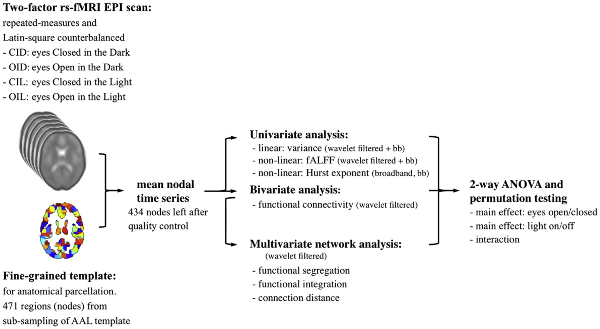
Schematic of the fMRI analysis pipeline. EPI data were preprocessed, coregistered into standard MNI space, and parcellated anatomically using a template image derived by sub-sampling the regions defined by the automated anatomical labeling (AAL) template. Each nodal time series was then analyzed with univariate, bivariate, and multivariate approaches by using the broadband time series before wavelet transformation and/or the wavelet filtered data. Between-condition differences were assessed by permutation testing controlled for repeated measures on within-subject factors.

Materials and methods

Sample

16 healthy right-handed volunteers (8 male, 8 female) were recruited by local advertising on campus (mean age=26.75 years; standard deviation 5.1 years). All subjects were screened by a questionnaire and a board-certified neurologist to exclude possible history of neurological illness, psychiatric disorders, or current drug use. Informed written consent was obtained from all participants in agreement with the protocol approved by the National Taiwan University Institutional Review Board.

Experimental design

Each subject underwent four separate scanning sessions under the following conditions: (1) eyes closed in darkness, CID; (2) eyes open in darkness, OID; (3) eyes closed in light, CIL; and (4) eyes open in light, OIL. The order of scanning under these conditions was counterbalanced across subjects by a Latin square design. Each of the scanning sessions lasted for 8 minutes with a few minutes of break between sessions. During the eyes open conditions, subjects were instructed to blink normally but keep their eyes open; during the eyes closed condition they were instructed not to fall asleep. During the conditions of darkness, we created a completely dark environment by covering the window of the MRI scan room meticulously with opaque black canvas. We also draft-proofed the door and covered the bore of the MRI machine tunnel. Any other dim light sources, like the buttons on the machine console, were also covered during the scan. Opaque lightproof goggles were not used because they did not match perfectly with each participant’s face but imposed additional physical constraint on the subjects. When all lights were off in the covered MRI scan room, the illumination was 0.000 cd/m² as measured by a digital Tektronix J17 Lumacolor photometer (Tektronix, Inc., Oregon, United States), while it was 27.41±2.36 cd/m2 just outside the bore of the MRI magnet when all lights were on.

FMRI data acquisition

Anatomical MRI data were first acquired from all subjects using a rapid acquisition with relaxation_T1 (RARE_T1) sequence on a 3.0 Tesla Medspec S300 scanner (Bruker Medical, Ettlingen, Germany). Resting state fMRI data were acquired using a gradient-echo echo-planar imaging (GE-EPI) sequence sensitive to BOLD contrast. Functional images were collected parallel to the AC-PC (anterior commissure– posterior commissure) plane with whole brain EPI acquisition from vertex to cerebellum. For all participants, we acquired 192 volumes in each condition with the following parameters: number of slices=30 (interleaved); slice thickness=4.5 mm; interslice gap=0 mm; matrix size=64×64; in-plane resolution=4.0×4.0 mm²; flip angle=90°; repetition time (TR)=2500 ms; echo time (TE)=30 ms.

FMRI data preprocessing and parcellation

The first 4 volumes of each EPI data set were discarded to allow for T1 saturation effects, leaving 188 volumes per session for time series and functional connectivity analysis. All data sets were preprocessed using SPM8 software (Wellcome Trust Center for Neuroimaging, University College London, www.fil.ion.ucl.ac.uk/spm). Pre-processing operations included slice-timing correction, head-motion correction using six rigid-body motion parameters, and normalization to the MNI (Montreal Neurological Institute) EPI template. After preprocessing, the image volume had a voxel size of 2×2×2 mm³.

No significant differences were noted between the four conditions regarding the mean head displacement (first temporal derivatives), maximum head displacement, the number of micro movements (>0.1 mm), and head rotation (Power et al., 2011; Van Dijk et al., 2011). For details, please see head motion parameters in the Supplementary Material. Each voxel time series was corrected for head movement by realignment and regression on the estimated head translations and rotations. We did not use global mean regression as part of the pre-processing applied to these data because this is currently considered to be a controversial step in fMRI data pre-processing. Some researchers have advocated global mean regression and consequently described correlated and anticorrelated networks (Fox et al., 2005b, 2009); however, other researchers have argued that the existence of strong anti-correlations (or negative correlations) is an artifact induced by global mean regression and it is therefore preferable not to include this step as part of fMRI time series pre-processing (Murphy et al., 2009; Weissenbacher et al., 2009).

The data were then spatially parcellated into 471 anatomical regions of interest, covering the cerebral hemispheres and cerebellum, using a template image derived by sub-sampling the larger regions defined by the automated anatomical labeling (AAL) template image (Tzourio-Mazoyer et al., 2002) to define a finer-grained parcellation with all regional parcels or nodes comprising an approximately equal number of voxels (Zalesky et al., 2010). Then, in each data set, we estimated the regional mean time series by averaging all voxel time series within each node. We excluded from further analysis those regions which had low EPI intensity (b2000) and/or low time series variance in one or more of the individual scans under any experimental condition. 37 regional nodes were excluded on this basis: these were located in areas prone to susceptibility artefact such as the orbitofrontal cortex, the inferior temporal cortex, and the brainstem. The pre-processed regional mean time series for the remaining 434 regional nodes in each individual dataset were used for further analysis.

Wavelet decomposition

Wavelet decomposition is widely used for filtering non-task fMRI cortical time series (Achard et al., 2006; Bullmore et al., 2004; Lynall et al., 2010; Maxim et al., 2005). It was implemented here using the WMTSA wavelet toolkit (Wavelet Methods for Time Series Analysis. Cornish, 2006. http://www.atmos.washington.edu/~wmtsa/, based on Percival and Walden, 2000). We used a maximal overlap discrete wavelet transform (MODWT) with a Daubechies 4 wavelet to decompose all individual regional mean time series into the following four scales (frequency intervals): scale 1 (0.1–0.2 Hz); scale 2 (0.05–0.1 Hz); scale 3 (0.025–0.05 Hz), and scale 4 (0.0125–0.025 Hz).

For functional connectivity and network construction in this study, wavelet scale 1 (0.1–0.2 Hz) fell in the higher frequency range considered to be contaminated by respiratory signals and usually not used for resting-state fMRI analysis (Biswal et al., 1995; Cordes et al., 2001). We therefore only used scales 2–4 data (0.0125–0.1 Hz) for analysis. We emphasized in particular scale 3 (0.025–0.05 Hz) because this frequency band has been previously associated with significant functional connectivity (Achard et al., 2006; Biswal et al., 1995; Fox and Raichle, 2007) and coincided with the frequency band having most of the power of spontaneous activity in visual areas during rest (<0.05 Hz) (Bianciardi et al., 2009; Cordes et al., 2001; Horovitz et al., 2008). For univariate time series analysis except the Hurst exponent (see method below), we used both the broadband time series before wavelet transformation and the wavelet filtered data (for estimation of fALFF, the broadband data was used as the denominator).

Univariate time series analysis

To characterize the variability of each fMRI time series in the time domain, we measured the variance of the BOLD signal, as well as the extent of its randomness and self-similarity as characterized by the Hurst exponent. In the frequency domain, we estimated the power of each time series in specific frequency bands by calculating the fractional amplitude of low frequency fluctuation (fALFF). The local (nodal) measure came from analyzing the mean data in each region (as defined by parcellation); we then calculated the mean of all nodal values to yield the global value.

Variance of the BOLD signal

For each pre-processed broadband time series or wavelet filtered data (X) we used the unbiased estimator of the variance with Bessel’s correction:

$$\text{Var}(X)=E\left({(X-\overline{X})}^2\right)=\frac{1}{n-1}\sum _{i=1}^n{\left(x_i-\overline{X}\right)}^2.$$ (1)

In addition to wavelet filtered data, we also used broadband data for calculating the variance of the BOLD signal, for the following two reasons. First, contrary to rs-fMRI functional connectivity and network analysis that generally avoid high frequency range data, there have been less discussions and thus less restraints about the calculation of variance of the BOLD signal. Second, it allows us to compare BOLD signal variance with other univariate parameters calculated based on the broadband data.

Frequency spectrum analysis (fALFF)

To estimate the fractional amplitude of low frequency fluctuation (fALFF) of each time series, we focused on the frequency spectrum between the Nyquist frequency 0.5×1/2.5=0.2 Hz and the lower limit of wavelet decomposition=0.0125 Hz. We first computed the amplitude for each frequency, then the sum of amplitudes across the wavelet scale 2 (0.05–0.1 Hz), scale 3 (0.025–0.05 Hz), and scale 4 (0.0125–0.025 Hz) frequency bands were divided separately by the sum of amplitudes across the full wavelet frequency spectrum of the time series, 0.0125–0.2 Hz. The Discrete Fourier Transform (DFT), X(k), of an N-point sequence x(n) is given by (Ingle and Proakis, 2011; Oppenheim et al., 1983):

$$X(k)=\sum _{n=0}^{N-1}x(n)W_N^{nk},0\le k\le N-1\text{\hspace{1em}using \hspace{1em}}{W}_N\triangleq e^{-j\frac{2\pi }{N}}.$$ (2)

Hurst exponent (H)

To further characterize the randomness and self-similarity of each time series, we used a wavelet-based estimator of the Hurst exponent (which takes broadband time series as input). A value of 0.5<H<1.0 represents positively autocorrelated or persistent behavior; 0<H<0.5 demonstrates negatively autocorrelated or anti-persistent behavior; H=0.5 corresponds to classical Gaussian white noise; and a smaller H suggests a more complex system (DePetrillo et al., 1999; Fan et al., 2009; Goldberger et al., 2002; Maxim et al., 2005; Natarajan et al., 2004). This provides a useful single parameter for non-stationary stochastic processes with long-term dependencies (Flandrin, 1992; Maxim et al., 2005).

Bivariate time series analysis

Functional connectivity

A set of {434×434} association matrices were obtained for each session and for each subject, by calculating the Pearson product moment correlation coefficient (r) between each regional pair of wavelet filter coefficients {X_i, Y_j} for the 434 regions (nodes, N) at wavelet scales 2, 3, and 4 respectively. The connectivity strength (S), also known as the weighted node degree, is the sum of correlations between index region i and all other regions. Then, the S at the global level for each subject, a.k.a. average weighted degree, is obtained from the mean of all nodal values:

$$r=\frac{Cov(X,Y)}{\sqrt{\text{Var}(X)\cdot \text{Var}(Y)}}=\frac{{\sum }_{i=1}^n\left(X_i-\overline{X}\right)\left(Y_i-\overline{Y}\right)}{\sqrt{{\sum }_{i=1}^n{\left(X_i-\overline{X}\right)}^2}\sqrt{{\sum }_{i=1}^n{\left(Y_i-\overline{Y}\right)}^2}},S(i)={\sum }_j{r}_{i,j}.$$ (3)

We calculated the confidence interval (C.I.) of correlation r for the pair of regions {i,j} across 16 subjects:

$$\text{C.I.}={\text{mean}}_{\text{boot}}\pm t\ast {\text{SE}}_{\text{boot}}$$ (4)

The mean_boot was the bootstrap mean of 20000 resamples of r, i.e., we randomly resampled with replacement the 16 individual subject estimates for each inter-regional correlation and calculated the mean of these bootstrap samples. t was the critical value for a one-tailed P-value=0.001 on 15 degrees of freedom, obtained from a standard distribution of t values. P-value was calculated from (1/N)/2=(1/434)/2=(0.0023/2)~0.001 (please see hypothesis testing for details). The 99.8% confidence interval for each inter-regional correlation was then constructed as the bootstrap mean±t×the bootstrap standard error of the mean (Moore, 2011). Under the null hypothesis that there was no correlation between different regions, we inferred that the correlation r was significant on average over participants if its 99.8% confidence interval did not include zero. The sign of the correlations was retained for the tests in order to demonstrate any significant negative correlations.

Multivariate functional network topology analysis

We constructed binary unweighted brain networks from each of the scales 2–4 absolute wavelet correlation matrices. Although the sign of the correlations was retained for the two-tailed tests of inter-regional correlations, we used the absolute correlation for the network analysis. As expected from previous studies by our group and others, most of the negative correlations were close to zero and not statistically significant, while most of the significant correlations were positively signed. This is typical of correlational estimates of fMRI connectivity, in our experience, unless the data have been preprocessed by regression of the global mean, which shifts the centre of the correlation distribution closer to zero and increases the proportion of large negative correlations in the distribution. Given that the correlation distribution was positively skewed in these data, and that graph analysis is complicated by signed measures of association between nodes, we considered it appropriate to use the absolute correlation matrix as the basis for graph construction. This approach has been previously used by our group and others in several prior studies (Achard and Bullmore, 2007; Achard et al., 2006; Lynall et al., 2010; Meunier et al., 2009a, 2009b).

To prevent the networks from becoming disconnected at very low connection density (sparsity), we used the minimum spanning tree (MST) as the backbone of the graph (Alexander-Bloch et al., 2010; Hagmann et al., 2008; Kruskal, 1956), and added additional edges as defined by a gradually decreasing global threshold to construct adjacency matrices of arbitrary connection density. That is, we added additional edges on the backbone of the graph according to the descending order of the weight of each edge. Many neuroscientists focus on relatively low connection densities (mostly <30%) because the topology of such sparse graphs is less random and more small-world (Achard et al., 2006; Alexander-Bloch et al., 2010; Bassett and Bullmore, 2009; Bassett et al., 2009; Ginestet et al., 2011; Lynall et al., 2010) and probably more biological in origin (Kaiser and Hilgetag, 2006). However, some macaque studies demonstrated that a greater range of connection density (up to 66%) is probably more realistic (Felleman and Van Essen, 1991; Markov et al., 2010). We calculated whole brain network topology metrics over a wide range of connection densities from 1% to 70% in 1% increments because network topology generally changes as a function of connection density and we considered it important to demonstrate that any factorial effects on network topology were robust to the arbitrary choice of connection density.

A detailed definition of the network measures of functional segregation and integration we used can be found in the supplementary materials section. Briefly we measured the clustering coefficient (Watts and Strogatz, 1998), the local efficiency (Latora and Marchiori, 2001), and the modularity (Newman, 2004) which are representative of segregated network topology; the characteristic path length (Watts and Strogatz, 1998) and the global efficiency (Latora and Marchiori, 2001) which are representative of integrative network topology; small-worldness, a measure of the balance between functional network segregation and integration (Watts and Strogatz, 1998), and the connection distance, a measure of information processing within the network (Sepulcre et al., 2010). All measures were calculated in Matlab using the Brain Connectivity Toolbox (see Rubinov and Sporns, 2010. http://www.brain-connectivity-toolbox). Connection distance (D) was calculated as the Euclidean distance between the centroids in physical space of each pair of regional nodes (i,j). At each density for each node, the nodal mean connection distance was the average Euclidean distance over all edges connecting the node to the rest of the network. The global mean connection distance or wiring cost was calculated as the average Euclidean distance over all pairs of connected nodes in the network (Alexander-Bloch et al., 2012; Sepulcre et al., 2010). Network metrics were compared at each connection density for wavelet scales 2–4.

For formal ANOVA modeling of factorial effects, we focused on the range from 5% to 30% connection density. We used a maximum of 30% connection density for these formal analyses because the prior exploratory analyses had confirmed (as others have shown previously; Achard and Bullmore, 2007; Achard et al., 2006) that at connection density greater than 30% approximately, brain fMRI networks tend to become dominated by random edges, as less strongly correlated edges are included at lower thresholds, and their complex topological properties are attenuated. To ensure that the results of ANOVA modeling were not conditioned on the choice of a single arbitrary threshold or connection density, we used the average of each topological metric over this range of connection density as the dependent variable (Ginestet et al., 2011).

Factorial analysis and hypothesis testing

We used a two-factor saturated ANOVA model (Doncaster and Davey, 2007) to examine the significance of the factorial effects of eyes open/closed and light on/off on each metric at the nodal (regional) and global (whole brain) levels of analysis.

We tested the main effects and the interaction for statistical significance using the F distribution. For tests of factorial effects on global measures of time series dynamics, connectivity and topology we used an uncorrected threshold P-value<0.05. For analysis of factorial effects on nodal (regional) measures, we controlled the probability of type I error for the number of comparisons involved in nodal analysis (P-value<1/N=1/434=0.0023). Although this false-positive correction is not as stringent as the Bonferroni correction, it is equivalent to saying that we expect less than one false-positive nodal test per cortical map (Alexander-Bloch et al., 2012; Bassett et al., 2009; Bullmore et al., 1999; Lai et al., 2010; Lynall et al., 2010).

Although violations of the assumption of normality do not strongly affect the validity of the ANOVA (Glass et al., 1972; Weinberg and Abramowitz, 2008), not all our data were normally distributed. We therefore verified the results of parametric testing by also conducting nonparametric tests based on permutation of the observed data. Using the same ANOVA model, each permutation was chosen by resampling without replacement and the probability distribution associated with the null hypothesis was sampled by estimating the F statistic after each of 20000 permutations of the data. The permutation procedure was also controlled for repeated measures on within-subject factors (Anderson, 2001; Cohen, 2008; Moore et al., 2011; Suckling et al., 2006; Weinberg and Abramowitz, 2008; see Supplementary Materials for details). Post-hoc two-tailed paired t-tests between different conditions were conducted using permutation testing only if the corresponding null hypothesis was rejected at factorial level. For sake of clarity, only the results of nonparametric statistical tests will be reported here.

All computations and statistical analyses were carried out in Matlab (Mathworks Inc., http://www.mathworks.com/), and graphics were plotted in Matlab or R (R Development Core Team. http://www.R-project.org/).

Cortical surface rendering

Caret v5.616 software was used for cortical surface visualization (Van Essen, 2005; Van Essen et al., 2001). In each cortical surface map of nodal statistics, the median value of the 16 subjects is rendered as representative of the experimental cohort.

Results

Factorial effects on univariate time series statistics

At both the global (whole brain) and nodal (regional) levels, eyes open/closed significantly affected the variance of the BOLD signal, the fractional amplitude of low frequency fluctuation (fALFF), and the Hurst exponent (H). However, neither the main effect of light on/off nor the interaction between eyes open/closed and light on/off was significant at either the global or nodal levels.

Variance of the BOLD signal

At the global level, eyes closed states including the CID (closed in the dark) and the CIL (closed in the light) conditions generally had higher variance of the BOLD signal, and ANOVA revealed that the main effect of eyes open/closed was significant (factorial permutation P-value=0.0004 at the global level for broadband data; 0.0012 for scale 2 data; 0.0007 for scale 3 data; 0.0069 for scale 4 data). In contrast, the main effect of light on/off was not significant (P-value=0.87 for broadband data; 0.65 for scale 2 data; 0.75 for scale 3 data; 0.84 for scale 4 data) while the interaction between eyes open/closed and light on/off had marginal effect on the variance of the BOLD signal (P-value=0.045 for broadband data; 0.0071 for scale 2 data; 0.033 for scale 3 data; 0.098 for scale 4 data) (see Fig. 2. for results of broadband and scale 3 data; Supplementary Material Fig. 1 for results of scales 2 and 4).

Fig. 2.

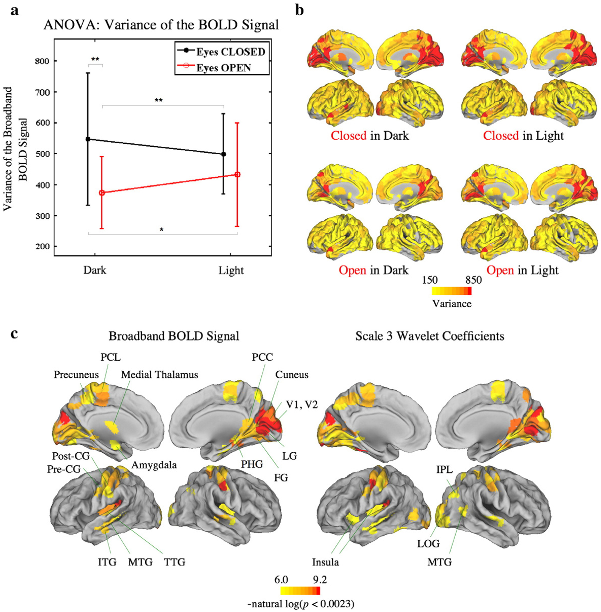
ANOVA and post-hoc analysis of variance of the BOLD signal at the global (whole brain) and nodal (regional) level. (a) Global level ANOVA and post-hoc pairwise analysis of broadband or unfiltered fMRI data. Eyes open or closed conditions strongly influenced the variance of the BOLD signal. (b) Median variance of the BOLD signal of all four conditions. The bilateral visual cortex, bilateral posterior cingulate cortex (PCC) and part of the bilateral precuneus showed higher variance of the BOLD signal. (c) Permutation tests at the nodal level for the main effect of eyes open/closed. Regions with a statistically significant main effect are highlighted. Results using time series before (left) or after (right) wavelet decomposition were quite similar. There were no statistically significant effects at nodal level of light on/off or the interaction between eyes open/closed and light on/off. Error bars show mean±SD. *P<0.05, **P<0.01, and ***P<0.001.

At the nodal level, there were apparent differences in the variance of the BOLD signal between different conditions. Variance was higher in the eyes closed conditions in most brain regions, with an emphasis on the bilateral visual cortex, bilateral posterior cingulate cortex (PCC, especially the isthmus part), and part of the bilateral precuneus (Fig. 2b).

Factorial permutation tests at the nodal level confirmed that the eyes closed state had a significantly higher variance of the BOLD signal than the eyes open state in the bilateral striate visual cortex (V1), the bilateral extrastriate visual cortex (bilateral V2, V3, V4, and right V5), the bilateral somatomotor and somatosensory cortex, and the left primary auditory cortex. In addition, the bilateral lingual gyrus, fusiform gyrus, parahippocampal gyrus, insula, and the left thalamus and amygdala were also affected in the same way (all significant P-valuesb(1/N)=0.0023 at the nodal level). However, there were no statistically significant effects at nodal level of light on/off or the interaction between eyes open/closed and light on/off. Note that, the results using time series before or after wavelet decomposition were very similar for all these analyses (see Fig. 2c for results of broadband and scale 3 data).

Fractional amplitude of low frequency fluctuation (fALFF)

At the global level, eyes closed states including the CID and CIL conditions generally had higher fALFF, and this effect was more obvious in the lower frequency bands including the wavelet scale 3 (0.025–0.05 Hz) and scale 4 (0.0125–0.025 Hz). Again, we found that it was eyes open/closed (P-value=0.52 for scale 2; 0.0061 for scale 3; 0.044 for scale 4) rather than light on/off (P-value=0.56 for scale 2; 0.39 for scale 3; 0.84 for scale 4) or interaction between eyes open/closed and light on/off (P-value=0.077 for scale 2; 0.35 for scale 3; 0.53 for scale 4) that had greatest effects on the fALFF (see Fig. 3a for results of wavelet scale 3, and Supplementary Material Fig. 2 for results of wavelet scales 2 and 4).

Fig. 3.

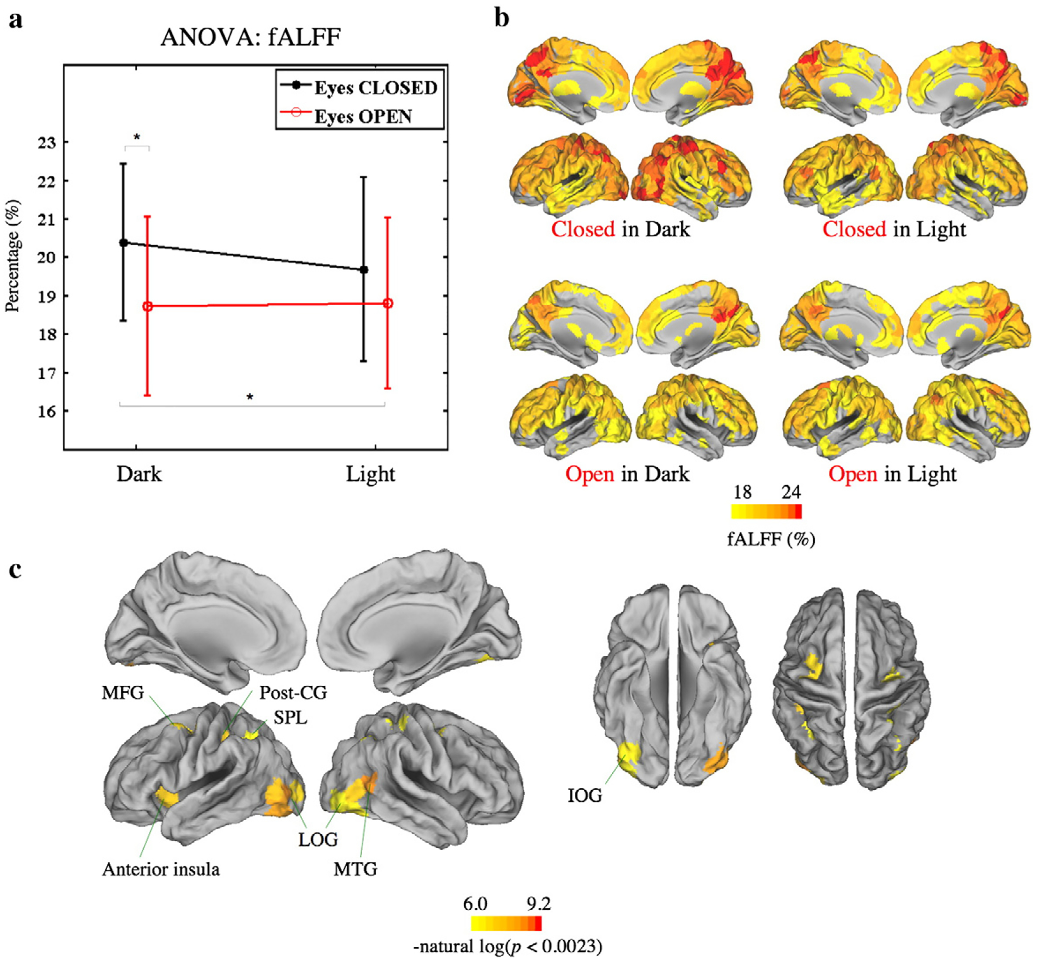
ANOVA and post-hoc analysis of the fALFF at the global and the nodal level, for wavelet scale 3. (a) Global level ANOVA and post-hoc pairwise analysis. Eyes closed states generally had higher fALFF, and fALFF was only affected by the eyes open/closed factor, independently of the light on/off factor or the interaction between the two. (b) Median variance of the fALFF of all four conditions. (c) Permutation tests at the nodal level for the main effect of eyes open/closed. Significant effects are visible in the secondary but not the primary visual cortex. There were no statistically significant nodal tests for the effect of light on/off or the interaction. Error bars show mean±SD. *P<0.05, **P<0.01, and ***P<0.001.

For wavelet scale 3 data at the nodal level, the eyes closed condition caused significantly higher fALFF (P-values<0.0023) in posterior brain regions including the bilateral lateral occipital gyrus, inferior occipital gyrus, postcentral gyrus, superior parietal lobule, and the right middle temporal gyrus and the left anterior insula. There were no statistically significant nodal effects of light on/off or the interaction between factors (Figs. 3b, c).

Hurst exponent

Only broadband time series were used in the analysis of the Hurst exponent. At the global level, ANOVA once more revealed that only the eyes open/closed factor influenced the Hurst exponent (Fig. 4a; permutation P-value=0.0321 for eyes open/closed at the global level). At the nodal level of analysis, however, there were no significant factorial effects on the Hurst exponent. Nevertheless there was, under each condition, a significant positive correlation between the variance of the BOLD signal and the Hurst exponent (CID state had r=0.27 with P-value=5.7×10⁻⁹; OID r=0.16 with P-value=7.0×10⁻⁴; CIL r=0.32 with P-value=1.6×10⁻¹¹, and OIL r=0.23 with P-value=1.4×10⁻⁶) (Fig. 4b). In addition, in all experimental conditions, there was a strong tendency for regions with high variance and positively autocorrelated time series to be located in the medial and posterior brain areas; regions with low variance and positively autocorrelated time series to be located in the lateral and anterior brain areas; regions with low variance and negatively autocorrelated time series to be located in the basal brain areas; while few regions had high variance and negatively autocorrelated time series (Fig. 4c).

Fig. 4.

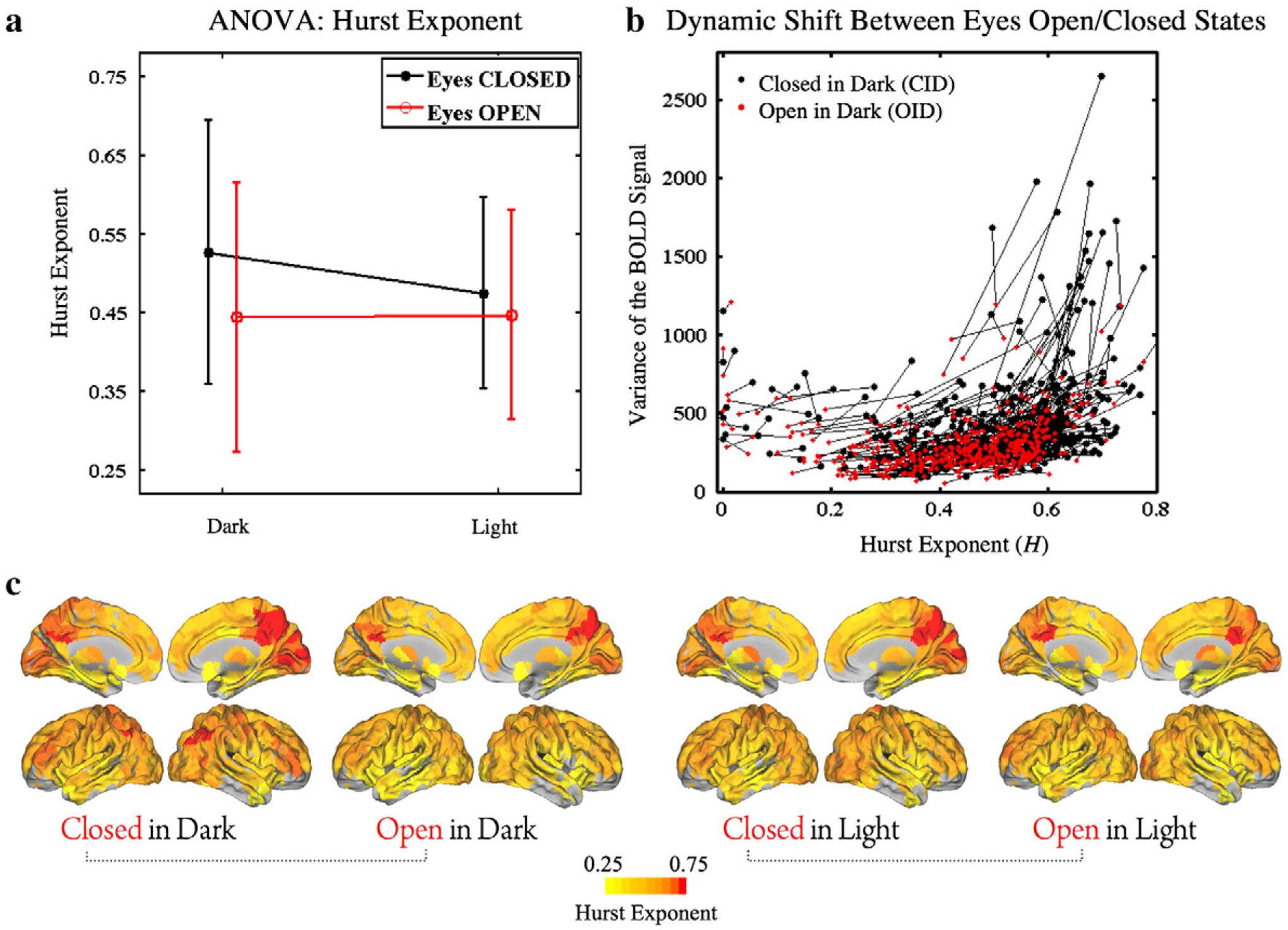
ANOVA and post-hoc analysis of the Hurst exponent at the global and the nodal level. (a) Global level ANOVA revealed that only the eyes open/closed factor influenced the Hurst exponent. However, no significant post-hoc paired t-tests were noted. Error bars show mean±SD. (b) Both the variance of the BOLD signal and the Hurst exponent tended to decrease when participants shifted from the eyes closed state to the eyes open state one (data plotted for a representative individual). (c) Median nodal Hurst exponent for all four conditions. The medial and posterior brain areas tended to have higher Hurst exponents.

Factorial effect on bivariate time series statistics

Functional connectivity

For wavelet scale 3 which had the most significant differences between eyes open/closed states among the univariate time series analyses, there were no significant factorial effects on strength of functional connectivity at the global level. At the nodal level, regions with higher connectivity strengths were located in the bilateral medial and posterior brain areas. Functionally, these were primary and secondary sensory cortical areas (Baehr et al., 2005), components of the limbic system, and deep brain regions like the medial thalamus. On the contrary, regions responsible for higher cognitive functions like the prefrontal and tertiary parietal association areas usually had much lower connectivity strengths (Fig. 5a). Nodal permutation tests of the main effect of eyes open/closed showed that the connectivity strength of the left frontal eye field (FEF, P-value=0.0008) and bilateral posterior cingulate cortex (Right PCC, P-value=0.0022; Left PCC, P-value=0.0022) decreased significantly during eyes open states (Fig. 5b).

Fig. 5.

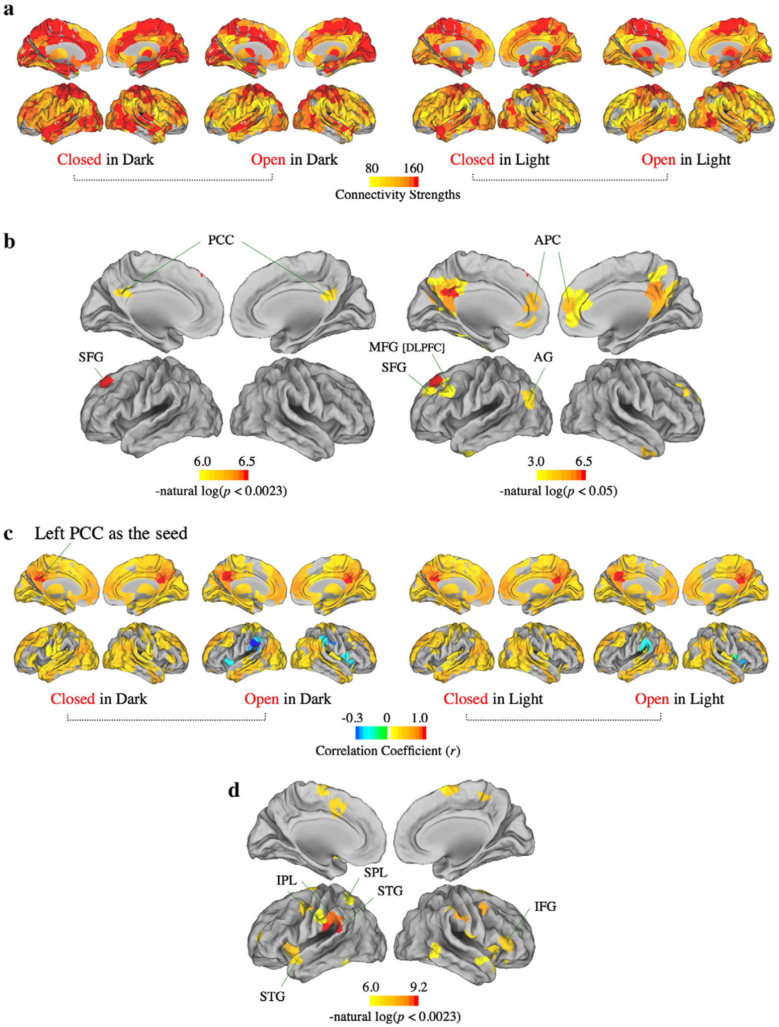
Connectivity strengths at the nodal level, and functional connectivity map, for wavelet scale 3. (a) Median nodal connectivity strengths for all four conditions. (b) Permutation tests of the main effect of eyes open/closed on connectivity strength at the nodal level. The functional connectivity strengths of the left frontal eye field (FEF) and bilateral posterior cingulate cortex (PCC) decreased significantly during eyes open states. This is shown at various statistical thresholds (left panel, P<0.0023; right panel, P<0.05). (c) Map highlighting regions that demonstrated significant functional connectivity (FC) of the left posterior cingulate cortex (PCC). (d) Permutation tests of the main effect of eyes open/closed on left PCC connectivity. The significant regions are focused on the bilateral perisylvian and perirolandic regions.

Then, by using the left PCC as the seed, it had the strongest connection with the right PCC throughout all four experimental conditions (bootstrap mean r=0.9429 for CID; 0.9323 for OID; 0.9366 for CIL; 0.9384 for OIL). It also had strong connectivity with the bilateral dorsolateral prefrontal (DLPFC) and tertiary parietal association cortices. In the eyes closed states, the left PCC only had positive correlations with other regions, but in the eyes open states it correlated negatively with the perisylvian structures, especially the bilateral supramarginal gyri (SMG) and the bilateral anterior insula (Fig. 5c). The functional connectivity between the left PCC and the bilateral perisylvian and perirolandic regions decreased significantly during eyes open states (Fig. 5d). The right PCC had much the same connectivity pattern.

Similarly, the left FEF had a similar connectivity pattern to the PCC, with strong connectivity to the bilateral prefrontal cortex and the tertiary parietal association cortex. The correlation between the left FEF and the bilateral perisylvian and perirolandic regions also decreased significantly (P-value<0.0023) during eyes open states (see Supplementary Material Fig. 3).

Furthermore, the left medial thalamus which we identified as having significantly higher BOLD variance during eyes closed states (Fig. 2c. P-value=0.0010 for broadband; 0.0093 for scale 3) also had very strong functional connectivity with the contralateral medial thalamus throughout all four experimental conditions (bootstrap mean r=0.92 for CID; 0.90 for OID; 0.92 for CIL; 0.91 for OIL), as well as diffuse significant positive functional connectivity with most of the brain areas except primary sensory cortices (including the primary visual, the primary somatosensory, and the primary auditory cortex) in the eyes closed state. Permutation testing of factorial effects at the nodal level revealed that only the main effect of eyes open/closed was significant. The functional connectivity between the left medial thalamus and the bilateral primary visual cortex and the right premotor cortex significantly increased during eyes open states (For right primary visual cortex, bootstrap mean r=0.14 for CID; 0.34 for OID; 0.08 for CIL; 0.38 for OIL, and P-value=0.0014. For left primary visual cortex, bootstrap mean r=0.17 for CID; 0.34 for OID; 0.08 for CIL; 0.39 for OIL, and P-value=0.0022. For right premotor cortex, bootstrap mean r=0.14 for CID; 0.30 for OID; 0.21 for CIL; 0.35 for OIL, and P-value=0.0010. See Supplementary Material Fig. 4 for details).

Factorial effects on multivariate network topology

Interestingly, despite the widespread factorial effects of the eyes open/closed condition on univariate properties of the BOLD signal, here we found no significant factorial effects, at global or nodal level, at any of the wavelet scales, on any of the network topology measures we estimated (Supplementary Material Figs. 5 and 6). However, there was a significant effect of eyes open/closed on network connection distance (see Fig. 6 for results of wavelet scale 3, and Supplementary Material Fig. 7 for results of wavelet scales 2 and 4).

Fig. 6.

ANOVA and post-hoc analysis of the network connection distance at the global and the nodal levels, for wavelet scale 3. (a) Network connection distance for all four experimental conditions at the whole brain (global) level, from 1% to 70% connection density (with 1% increment in density at each step). The red asterisks signify an uncorrected P<0.05 for the permutation test of the main effect of eyes open/closed on connection distance. (b) Global level ANOVA and post-hoc pairwise analysis of the integral of connection distance over all connection densities between 5% and 30%. (c) Median variance of the connection distance of all four conditions at 20% connection density. (d) Permutation tests at the nodal level of the main effect of eyes open/closed main effect on connection distance in networks thresholded with 20% connection density. Eyes open/closed had a significant effect on the connection distance of left inferior parietal lobule (BA40), the left superior temporal gyrus (BA22), and the right superior parietal lobule (BA7). There were no significant effects of light on/off or the interaction between eyes open/closed and light on/off on connection distance. Error bars show mean±SD. *P<0.05, **P<0.01, and ***P<0.001. CID, eyes Closed In the Dark; OID, eyes Open In the Dark; CIL, eyes Closed In the Light; OIL, eyes Open In the Light; Ran, random.

The eyes open states including the open in dark (OID) and the open in light (OIL) conditions had longer connection distance than the eyes closed states (Fig. 6a). At the global level, ANOVA revealed that only the main effect of eyes open/closed significantly modulated the connection distance (permutation P-value=0.0361 for wavelet scale 2; P-value=0.0139 for wavelet scale 3; P-value=0.2190 for wavelet scale 4; see also Fig. 6b).

At the nodal level, the bilateral prefrontal and the parietal association cortex had longer connection distance than other regions. In addition, there was also a noticeable interhemispheric asymmetry with left pre-dominance (Fig. 6c). Permutation tests at the nodal level revealed that there was a significant main effect of eyes open/closed on the connection distance of the left inferior parietal lobule (BA40. P-value=0.00005), the bilateral superior temporal gyrus (BA22. Left side P-value= 0.0001; right side P-value=0.0016), and the right superior parietal lobule (BA7. P-value=0.0022) (Fig. 6d). Once again, there were no significant effects of light on/off, or the interaction between eyes open/ closed and light on/off on connection distance, at any wavelet scale.

Discussion

In this study, we expanded the traditional eyes open/closed experiment to a balanced, two-factored, repeated measures, resting state fMRI study to differentiate the influences on brain function caused by eyes open/closed from those due to light on/off. Our contributions are twofold. First, we demonstrated that the effects caused by volitional changes in eyes open or closed conditions were clearly independent of changes in the exogenous visual stimuli. Second, we analyzed these changes from a whole brain topological perspective and revealed their relationship with various univariate and bivariate time series metrics.

Physiologically, there are reflexive, spontaneous, and volitional (intentional) eye blinks. Reflexive and spontaneous eye blinks are controlled mainly by the brainstem circuits (Baehr et al., 2005; Schmidtke and Buttner-Ennever, 1992) and should, in principle, have little relationship with our study. Instead, our experimental design manipulates volitional changes in eyes open or closed conditions which are reported to have a strong correlation with deep brain structures, ascending reticular activating system (ARAS), motor system (Baehr et al., 2005; Brazis et al., 2007; FitzGerald and Folan-Curran, 2002), sensory systems (Goldman et al., 2002; Lorincz et al., 2009; Marx et al., 2003, 2004; McAvoy et al., 2008; Schreckenberger et al., 2004; Singh et al., 1998), emotional experience (Lerner et al., 2009), and higher cognitive functions (Colzato et al., 2008).

While recent literature has discussed various differences in brain function between eyes open and eyes closed states (using EEG, MEG and fMRI), to the best of our knowledge, we are the first to investigate the effects of these conditions in a formally counterbalanced factorial design. In general, we observe diffuse changes in the primary and secondary sensory cortical areas, the tertiary parietal association cortex, the default mode network, the thalamus, the amygdala, and the insula. Our finding that the eyes open/closed states affect in particular the visual cortex is compatible with the related alpha response observed in EEG/MEG studies (Berger, 1929; Goldman et al., 2002; Schreckenberger et al., 2004). Some specific anterior brain structures like the premotor cortex and the frontal eye field were also significantly affected. These findings might be helpful for further studies related to attention, (visual) consciousness, sleep, and mindful activities like meditation, because most of the above mentioned activities are related to changes in eyes open or closed states and some of them are initiated by and maintained in the eyes closed conditions.

Metrics of univariate, bivariate, and multivariate analyses in this study were significantly correlated (Fig. 7). These correlational analyses demonstrate that although these metrics measure different aspects of brain function they can nonetheless demonstrate correlated changes in response to changing experimental conditions and should not therefore be considered as independent brain functional markers. In what follows, we review and interpret in more detail the main results from each of the metrics we have used, in the context of the prior literature.

Fig. 7.

Correlation matrices between the mean of different fMRI global functional metrics for the Closed in the Dark (CID) condition, for wavelet scale 3 (Broadband data were used for the variance of the BOLD signal and Hurst exponent). Nonsignificant correlations (P>0.05) are left blank.

Firstly, we found higher variance in the BOLD signal for the eyes closed conditions, and the regions with a statistically significant main effect were similar to previous studies using power spectral density (McAvoy et al., 2008) and blocked design general linear model (GLM) analysis (Marx et al., 2003). The variance of BOLD spontaneous fluctuations has previously been attributed to intrinsic brain activity, and is known to be relevant for or even to predict human perception and behavior (Fox et al., 2005a, 2007; Ramot et al., 2011; Wang et al., 2008). For example, Fox et al. demonstrated that trial-to-trial variability in the right somatomotor cortex (SMC) persisted during a right index-finger button press task and contributed to variability in evoked brain responses in the left SMC. As a result, variance changes brought about by a shift between eyes open and eyes closed conditions might consequently affect relevant evoked cognitive activities. Therefore, eyes open/closed may be treated as different “task states” or “control states”, and deserve more careful attention in design of resting-state and even other cognitive block or event-related experiments.

Fractional amplitude of low frequency fluctuation (fALFF) is also a widely used biomarker for brain physiological states (Yang et al., 2007; Zou et al., 2008, 2010). Interestingly, fALFF changes caused by eyes open/closed conditions were distributed in the secondary but not the primary visual cortex. This implies that even without visual stimulation, the secondary visual cortex reacted to simple eyes open/closed changes. In addition, the results of fALFF analysis emphasized the fact that changes in eyes open or closed conditions also affect sensory systems other than the visual system. For example, it was notable that the left anterior insula had higher fALFF during eyes closed states. Given that the anterior insula is involved in interoception, subjective feelings, and awareness (Bud Craig, 2009), our results reinforce the role of changes of eyes open or closed conditions in generally modulating human perception and cognitive function.

It is worth mentioning that prior literature using ALFF in the frequency range of 0.01–0.08 Hz in specific ROIs (6 slices covering the visual cortex, PCC, and sensorimotor cortex) has reported that ALFF to be lower in the eyes closed than in the eyes open state (Yang et al., 2007). The discrepancy between this work and our results may be attributable to several reasons. Firstly, the fALFF measure used here is less sensitive to physiological noise than ALFF. Secondly, we found that the trend of fALFF is not completely consistent between different frequency bands, with scale 3 and scale 4 showing the most significant changes. This phenomenon could therefore be obscured in a wider range ALFF analysis. Thirdly, whole brain analyses and studies involving specific ROIs will inevitably have differing statistical power. However, more evidence is needed to clarify this point.

As a final univariate measure, we considered the Hurst exponent, a fractal scaling property measuring self-similarity, and complexity. While this measure was dynamic and region-specific, we also found it to be relatively robust in normal healthy subjects. The trend for the eyes closed states to have a higher Hurst exponent — more positive autocorrelation with less non-linear complexity — especially in the visual cortex is arguably compatible with the strong alpha rhythm observed in EEG studies under eyes closed conditions (Berger, 1929; Goldman et al., 2002; Natarajan et al., 2004; Schreckenberger et al., 2004). Importantly, our results imply that the increase of complexity during eyes open states is entirely endogenous and independent of exogenous visual stimulation.

Our findings are also compatible with the concept that lying quietly with eyes closed corresponds to the brain’s baseline state or the default mode (Raichle et al., 2001). The DMN involving PCC, precuneus (PCu), medial prefrontal cortex (MPFC), ventral anterior cingulate cortex (vACC), and bilateral inferior parietal cortex (IPC) has been studied extensively using resting-state fMRI (Fox et al., 2005b; Greicius et al., 2003; Raichle et al., 2001). In addition, various components of the DMN, especially in the posterior brain, are known to be involved in sensory processing. For instance, the PCC is linked to cortical areas with visual, auditory, somatosensory, and oculomotor functions (Arnott et al., 2008; Nobre et al., 1997; Olson and Musil, 1992) — a point which is likely relevant to our findings as well as to related results in recent literature (Yang et al., 2007; Zou et al., 2009). Our results highlight the care that needs to be taken when comparing the DMN obtained across studies with eyes open and eyes closed conditions.

Upon examining these brain functional networks we noted that regions responsible for higher cognitive activities like the prefrontal and the parietal association cortex usually had longer connection distance. This phenomenon persisted across the four conditions and was in agreement with previous literature (Sepulcre et al., 2010). In addition, we found that the mean connection distance of all regions increased during the eyes open states. The regions where this effect was most significant were the association cortices including the left inferior parietal lobule, the left superior temporal gyrus, and the right superior parietal lobule. This finding is compatible with the point of view that the eyes closed condition is the ‘resting’ state, and that increased connection distance during the eyes open state reflects a reconfiguration of the economical brain network to include higher cost long-distance connections in order to support the greater information processing requirements of the eyes open condition (Alexander-Bloch et al., 2012; Niven and Laughlin, 2008).

Despite the significant effects of the eyes open/closed condition on the univariate and bivariate properties of the BOLD signal described above, in this study, the multivariate network topology metrics other than the connection distance were relatively invariant under all four experimental conditions. One potential explanation for this is that variations in the univariate properties of the signal may not affect the pairwise correlation values defining the network — in other words, the inter-relationship between time series of different regions may remain stable. Our results on connectivity strength (and on connection distance) (Figs. 5 and 6) however suggest that this is not the case for the networks considered here. Instead, we conclude that while the connectivity of individual edges is indeed affected by the various experimental conditions, the global network metrics examined here lack the sensitivity to detect these changes. These results suggest that the global network metrics of the traditional network analyses risk overlooking certain important physiological effects. On the other hand, this relative insensitivity means that any significant changes in network metrics, such as those observed in various disease states, represent remarkable changes in BOLD time series properties as well as the underlying physiological states.

Vision is the only sensation that can be interrupted volitionally in a natural way. Independently of the visual input, we demonstrate that human brain networks adopt a distinctive configuration when eyes are open (compared to when eyes are closed), i.e., under conditions when visual input might normally be expected. Although it is well known that visual input stimulates the brainstem, thalamus, and visual cortex, induces wakefulness through the ascending reticular activating system (ARAS) (Brazis et al., 2007; FitzGerald and Folan-Curran, 2002), and mediates various higher cognitive functions (Itti and Koch, 2001), we found no significant effects of light on/off, nor was there any evidence for significant interactions between eyes open/closed and light on/off. One reasonable explanation is that these effects are relatively small and obscured by the stringent statistical threshold used to control for multiple comparisons. In other words, it is possible that the absence of effects of these factors is a type 2 error. Alternatively it is arguable that the contrast between light on and light off conditions in this experiment was not salient enough to evoke a significant change in brain function. However, the latter explanation is weakened by the fact that there was indeed a major difference between a completely visibly dark environment and one in which all subjects could see clearly. Nonetheless, our results clearly re-emphasize the important brain functional changes caused by the difference between volitional eyes opening and eyes closed conditions.

Some methodological aspects of the study should be mentioned. First, we did not apply a fixation point during eyes open conditions and this probably allowed a small amount of undesirable oculomotor behavior. However, lack of visual fixation was dictated by the requirement for a completely dark environment. Second, head motion can induce spurious functional connectivity (Power et al., 2011; Satterthwaite et al., 2012; Van Dijk et al., 2011). Since it is inevitable that even healthy volunteers produce detectable movements in the MRI scanner, we carefully analyzed multiple movement parameters in each image but were unable to demonstrate any significant differences prior to correction of movement related variance in all time series by regression.

Conclusion

We used a balanced, factorial design to study effects of eyes open or closed conditions on resting state fMRI. Eyes open and closed conditions by themselves were associated with significant changes in fMRI time series dynamics, functional connectivity, and connection distance of functional networks regardless of exogenous visual input. In light of these results, controlling for eyes open/closed is recommended for design of resting state fMRI experiments.

Abbreviations:

CID

eyes Closed In the Dark

OID

eyes Open In the Dark

CIL

eyes Closed In the Light

OIL

eyes Open In the Light

AG

Angular Gyrus

APC

Anterior Prefrontal Cortex

DLPFC

Dorsolateral Prefrontal Cortex

FEF

Frontal Eye Field

FG

Fusiform Gyrus

HG

Heschl’s Gyrus

IFG

Inferior Frontal Gyrus

IOG

Inferior Occipital Gyrus

IPL

Inferior Parietal Lobule

ITG

Inferior Temporal Gyrus

LOG

Lateral Occipital Gyrus

MFG

Middle Frontal Gyrus

MTG

Middle Temporal Gyrus

PCC

Posterior Cingulate Cortex

PCL

Paracentral Lobule

PHG

Parahippocampal Gyrus

Post-CG

Postcentral Gyrus

Pre-CG

Precentral Gyrus

SFG

Superior Frontal Gyrus

SPL

Superior Parietal Lobule

STG

Superior Temporal Gyrus

TTG

Transverse Temporal Gyrus

References

- Achard S, Bullmore E, 2007. Efficiency and cost of economical brain functional networks. PLoS Comput. Biol 3 (2). [DOI] [PMC free article] [PubMed] [Google Scholar]
- Achard S, et al. , 2006. A resilient, low-frequency, small-world human brain functional network with highly connected association cortical hubs. J. Neurosci 26 (1), 63–72. [DOI] [PMC free article] [PubMed] [Google Scholar]
- Alexander-Bloch AF, et al. , 2010. Disrupted modularity and local connectivity of brain functional networks in childhood-onset schizophrenia. Front. Syst. Neurosci 4. [DOI] [PMC free article] [PubMed] [Google Scholar]
- Alexander-Bloch AF, et al. , 2013. The anatomical distance of functional connections predicts brain network topology in health and schizophrenia. Cereb. Cortex 23 (1), 127–138. [DOI] [PMC free article] [PubMed] [Google Scholar]
- Anderson MJ, 2001. Permutation tests for univariate or multivariate analysis of variance and regression. Can. J. Fish. Aquat. Sci 58 (3), 626–639. [Google Scholar]
- Arnott SR, et al. , 2008. Voice recognition and the posterior cingulate: an fMRI study of prosopagnosia. J. Neuropsychol 2 (1), 269–286. [DOI] [PubMed] [Google Scholar]
- Baehr M, Frotscher M, Duus P, 2005. Duus’ topical diagnosis in neurology: anatomy, physiology, signs, symptoms. George Thieme Verlag. [Google Scholar]
- Barnes A, Bullmore ET, Suckling J, 2009. Endogenous Human Brain Dynamics Recover Slowly Following Cognitive Effort. PLoS One 4 (8), e6626. [DOI] [PMC free article] [PubMed] [Google Scholar]
- Bassett DS, Bullmore ET, 2009. Human brain networks in health and disease. Curr. Opin. Neurol 22 (4), 340–347. [DOI] [PMC free article] [PubMed] [Google Scholar]
- Bassett DS, et al. , 2009. Cognitive fitness of cost-efficient brain functional networks. Proc. Natl. Acad. Sci 106 (28), 11747–11752. [DOI] [PMC free article] [PubMed] [Google Scholar]
- Berger Hans, 1929. Über das Elektrenkephalogramm des Menchen. Arch. Psychiatr 87, 527–570. [Google Scholar]
- Bianciardi M, et al. , 2009. Modulation of spontaneous fMRI activity in human visual cortex by behavioral state. NeuroImage 45 (1), 160–168. [DOI] [PMC free article] [PubMed] [Google Scholar]
- Birn RM, Saad ZS, Bandettini PA, 2001. Spatial heterogeneity of the nonlinear dynamics in the FMRI BOLD response. NeuroImage 14 (4), 817–826. [DOI] [PubMed] [Google Scholar]
- Biswal B, et al. , 1995. Functional connectivity in the motor cortex of resting human brain using echo-planar MRI. Magn. Reson. Med 34 (4), 537–541. [DOI] [PubMed] [Google Scholar]
- Biswal B, et al. , 1997. Hypercapnia reversibly suppresses low-frequency fluctuations in the human motor cortex during rest using echo-planar MRI. J. Cereb. Blood Flow Metab 17 (3), 301–308. [DOI] [PubMed] [Google Scholar]
- Brazis PW, Masdeu JC, Biller J, 2007. Localization in Clinical Neurology Lippincott Williams & Wilkins. [Google Scholar]
- Bud Craig AD, 2009. How do you feel — now? The anterior insula and human awareness. Nat. Rev. Neurosci 10, 59–70. [DOI] [PubMed] [Google Scholar]
- Bullmore E, Sporns O, 2009. Complex brain networks: graph theoretical analysis of structural and functional systems. Nat. Rev. Neurosci 10 (3), 186–198. [DOI] [PubMed] [Google Scholar]
- Bullmore E, Sporns O, 2012. The economy of brain network organization. Nat. Rev. Neurosci 13 (5), 336–349. [DOI] [PubMed] [Google Scholar]
- Bullmore ET, et al. , 1999. ‘Global, voxel, and cluster tests, by theory and permutation, for a difference between two groups of structural MR images of the brain’, Medical Imaging. IEEE Trans. Med. Imaging 18 (1), 32–42. [DOI] [PubMed] [Google Scholar]
- Bullmore E, et al. , 2004. Wavelets and functional magnetic resonance imaging of the human brain. NeuroImage 23, S234–S249. [DOI] [PubMed] [Google Scholar]
- Cohen B, 2008. Explaining Psychological Statistics, 3rd ed. John Wiley & Sons. [Google Scholar]
- Colzato LS, et al. , 2008. Blinks of the eye predict blinks of the mind. Neuropsychologia 46 (13), 3179–3183. [DOI] [PubMed] [Google Scholar]
- Cordes D, et al. , 2001. Frequencies contributing to functional connectivity in the cerebral cortex in “resting-state” data. Am. J. Neuroradiol 22 (7), 1326–1333. [PMC free article] [PubMed] [Google Scholar]
- Cornish Charlie, 2006. WMTSA Wavelet Toolkit for MATLAB, 0.2.6 ed. University of Washington. [Google Scholar]
- DePetrillo PB, Speers A, Ruttimann UE, 1999. Determining the Hurst exponent of fractal time series and its application to electrocardiographic analysis. Comput. Biol. Med 29 (6), 393–406. [DOI] [PubMed] [Google Scholar]
- Doncaster CP, Davey AJH, 2007. Analysis of Variance and Covariance: How to Choose and Construct Models for the Life Sciences. Cambridge Univ Press. [Google Scholar]
- Fan Y, et al. , 2009. The effect of investor psychology on the complexity of stock market: an analysis based on cellular automaton model. Comput. Ind. Eng 56 (1), 63–69. [Google Scholar]
- Felleman DJ, Van Essen DC, 1991. Distributed hierarchical processing in the primate cerebral cortex. Cereb. Cortex 1 (1), 1–47. [DOI] [PubMed] [Google Scholar]
- Fisch BJ, Spehlmann R, 1999. Fisch and Spehlmann’s EEG Primer: Basic Principles of Digital and Analog EEG. Elsevier Science Health Science div. [Google Scholar]
- FitzGerald MJT, Folan-Curran J, 2002. Clinical Neuroanatomy and Related Neuroscience. WB Saunders Co. [Google Scholar]
- Flandrin P, 1992. ‘Wavelet analysis and synthesis of fractional Brownian motion’, Information Theory. IEEE Trans. Inf. Theory 38 (2), 910–917. [Google Scholar]
- Fox MD, Raichle ME, 2007. Spontaneous fluctuations in brain activity observed with functional magnetic resonance imaging. Nat. Rev. Neurosci 8 (9), 700–711. [DOI] [PubMed] [Google Scholar]
- Fox MD, et al. , 2005a. The human brain is intrinsically organized into dynamic, anticorrelated functional networks. Proc. Natl. Acad. Sci. U. S. A 102 (27), 9673–9678. [DOI] [PMC free article] [PubMed] [Google Scholar]
- Fox MD, et al. , 2005b. Coherent spontaneous activity accounts for trial-to-trial variability in human evoked brain responses. Nat. Neurosci 9 (1), 23–25. [DOI] [PubMed] [Google Scholar]
- Fox MD, et al. , 2007. Intrinsic fluctuations within cortical systems account for intertrial variability in human behavior. Neuron 56 (1), 171–184. [DOI] [PubMed] [Google Scholar]
- Fox MD, et al. , 2009. The global signal and observed anticorrelated resting state brain networks. J. Neurophysiol 101 (6), 3270–3283. [DOI] [PMC free article] [PubMed] [Google Scholar]
- Friston KJ, 1994. Functional and effective connectivity in neuroimaging: a synthesis. Hum. Brain Mapp 2 (1–2), 56–78. [Google Scholar]
- Fukunaga M, et al. , 2006. Large-amplitude, spatially correlated fluctuations in BOLD fMRI signals during extended rest and early sleep stages. Magn. Reson. Imaging 24 (8), 979–992. [DOI] [PubMed] [Google Scholar]
- Gilden DL, Thornton T, Mallon MW, 1995. 1/f noise in human cognition. Science 267 (5205), 1837–1839. [DOI] [PubMed] [Google Scholar]
- Ginestet CE, et al. , 2011. Brain network analysis: separating cost from topology using cost-integration. PLoS One 6 (7), e21570. [DOI] [PMC free article] [PubMed] [Google Scholar]
- Glass GV, Peckham PD, Sanders JR, 1972. Consequences of failure to meet assumptions underlying the fixed effects analyses of variance and covariance. Rev. Educ. Res 42 (3), 237–288. [Google Scholar]
- Goldberger AL, et al. , 2002. Fractal dynamics in physiology: alterations with disease and aging. Proc. Natl. Acad. Sci. U. S. A 99 (Suppl. 1), 2466. [DOI] [PMC free article] [PubMed] [Google Scholar]
- Goldman RI, et al. , 2002. Simultaneous EEG and fMRI of the alpha rhythm. NeuroReport 13 (18), 2487–2492. [DOI] [PMC free article] [PubMed] [Google Scholar]
- Greicius MD, et al. , 2003. Functional connectivity in the resting brain: a network analysis of the default mode hypothesis. Proc. Natl. Acad. Sci 100 (1), 253–258. [DOI] [PMC free article] [PubMed] [Google Scholar]
- Hagmann P, et al. , 2008. Mapping the structural core of human cerebral cortex. PLoS Biol 6 (7), e159. [DOI] [PMC free article] [PubMed] [Google Scholar]
- Horovitz SG, et al. , 2008. Low frequency BOLD fluctuations during resting wakefulness and light sleep: a simultaneous EEG fMRI study. Hum. Brain Mapp 29 (6), 671–682. [DOI] [PMC free article] [PubMed] [Google Scholar]
- Ingle VK, Proakis JG, 2011. Digital Signal Processing Using MATLAB. Thomson Engineering. [Google Scholar]
- Itti L, Koch C, 2001. Computational modelling of visual attention. Nat. Rev. Neurosci 2 (3), 194–203. [DOI] [PubMed] [Google Scholar]
- Jann K, et al. , 2009. BOLD correlates of EEG alpha phase-locking and the fMRI default mode network. NeuroImage 45 (3), 903–916. [DOI] [PubMed] [Google Scholar]
- Kaiser M, Hilgetag CC, 2006. Nonoptimal component placement, but short processing paths, due to long-distance projections in neural systems. PLoS Comput. Biol 2 (7), e95. [DOI] [PMC free article] [PubMed] [Google Scholar]
- Kiviniemi VJ, et al. , 2005. Midazolam sedation increases fluctuation and synchrony of the resting brain BOLD signal. Magn. Reson. Imaging 23 (4), 531–537. [DOI] [PubMed] [Google Scholar]
- Kruskal JB, 1956. On the shortest spanning subtree of a graph and the traveling salesman problem. Proc. Am. Math. Soc 7 (1), 48–50. [Google Scholar]
- Lai MC, et al. , 2010. A shift to randomness of brain oscillations in people with autism. Biol. Psychiatry 68 (12), 1092–1099. [DOI] [PubMed] [Google Scholar]
- Latora V, Marchiori M, 2001. Efficient behavior of small-world networks. Phys. Rev. Lett 87 (19), 198701. [DOI] [PubMed] [Google Scholar]
- Lerner Y, et al. , 2009. Eyes wide shut: amygdala mediates eyes-closed effect on emotional experience with music. PLoS One 4 (7), e6230. [DOI] [PMC free article] [PubMed] [Google Scholar]
- Li SJ, et al. , 2000. Cocaine administration decreases functional connectivity in human primary visual and motor cortex as detected by functional MRI. Magn. Reson. Med 43 (1), 45–51. [DOI] [PubMed] [Google Scholar]
- Liu Y, et al. , 2007. Whole brain functional connectivity in the early blind. Brain 130 (8), 2085–2096. [DOI] [PubMed] [Google Scholar]
- Lorincz ML, et al. , 2009. Temporal framing of thalamic relay-mode firing by phasic inhibition during the alpha rhythm. Neuron 63 (5), 683–696. [DOI] [PMC free article] [PubMed] [Google Scholar]
- Lynall ME, et al. , 2010. Functional connectivity and brain networks in schizophrenia. J. Neurosci 30 (28), 9477–9487. [DOI] [PMC free article] [PubMed] [Google Scholar]
- Markov N, et al. , 2010. ‘Principles of Inter-Areal Connections of the Macaque Cortex’, Neurocomp 2010. Lyon, France. [Google Scholar]
- Marx E, et al. , 2003. Eye closure in darkness animates sensory systems. NeuroImage 19 (3), 924–934. [DOI] [PubMed] [Google Scholar]
- Marx E, et al. , 2004. Eyes open and eyes closed as rest conditions: impact on brain activation patterns. NeuroImage 21 (4), 1818–1824. [DOI] [PubMed] [Google Scholar]
- Maxim V, et al. , 2005. Fractional Gaussian noise, functional MRI and Alzheimer’s disease. NeuroImage 25 (1), 141–158. [DOI] [PubMed] [Google Scholar]
- Mazoyer B, et al. , 2001. Cortical networks for working memory and executive functions sustain the conscious resting state in man. Brain Res. Bull 54 (3), 287–298. [DOI] [PubMed] [Google Scholar]
- McAvoy M, et al. , 2008. Resting states affect spontaneous BOLD oscillations in sensory and paralimbic cortex. J. Neurophysiol 100 (2), 922–931. [DOI] [PMC free article] [PubMed] [Google Scholar]
- McGonigle DJ, et al. , 2003. Variability in fMRI: an examination of intersession differences. IEEE; 27. [DOI] [PubMed] [Google Scholar]
- Meunier D, et al. , 2009a. Age-related changes in modular organization of human brain functional networks. NeuroImage 44 (3), 715–723. [DOI] [PubMed] [Google Scholar]
- Meunier D, et al. , 2009b. Hierarchical modularity in human brain functional networks. Front. Neuroinform 3. [DOI] [PMC free article] [PubMed] [Google Scholar]
- Moore DS, et al. , 2011. Introduction to the Practice of Statistics, 7th ed. W. H. Freeman. [Google Scholar]
- Murphy K, et al. , 2009. The impact of global signal regression on resting state correlations: are anti-correlated networks introduced? NeuroImage 44 (3), 893–905. [DOI] [PMC free article] [PubMed] [Google Scholar]
- Natarajan K, et al. , 2004. Nonlinear analysis of EEG signals at different mental states. Biomed. Eng. Online 3 (1), 7. [DOI] [PMC free article] [PubMed] [Google Scholar]
- Newman MEJ, 2004. Fast algorithm for detecting community structure in networks. Phys. Rev. E 69 (6), 066133. [DOI] [PubMed] [Google Scholar]
- Nir Y, et al. , 2006. Widespread functional connectivity and fMRI fluctuations in human visual cortex in the absence of visual stimulation. NeuroImage 30 (4), 1313–1324. [DOI] [PubMed] [Google Scholar]
- Niven JE, Laughlin SB, 2008. Energy limitation as a selective pressure on the evolution of sensory systems. J. Exp. Biol 211 (11), 1792–1804. [DOI] [PubMed] [Google Scholar]
- Nobre AC, et al. , 1997. Functional localization of the system for visuospatial attention using positron emission tomography. Brain 120 (3), 515–533. [DOI] [PubMed] [Google Scholar]
- Olson CR, Musil SY, 1992. Posterior cingulate cortex: sensory and oculomotor properties of single neurons in behaving cat. Cereb. Cortex 2 (6), 485–502. [DOI] [PubMed] [Google Scholar]
- Oppenheim AV, Willsky AS, Young IT, 1983. Signals and Systems. Prentice-Hal, Upper Saddle River, NJ. (796). [Google Scholar]
- Percival DB, Walden AT, 2000. Wavelet Methods for Time Series Analysis. Cambridge Univ Pr. (4). [Google Scholar]
- Power JD, et al. , 2011. Spurious but systematic correlations in functional connectivity MRI networks arise from subject motion. NeuroImage 59, 2142–2154. [DOI] [PMC free article] [PubMed] [Google Scholar]
- Pritchard WS, 1992. The brain in fractal time: 1/f-like power spectrum scaling of the human electroencephalogram. Int. J. Neurosci 66 (1–2), 119–129. [DOI] [PubMed] [Google Scholar]
- Raichle ME, et al. , 2001. A default mode of brain function. Proc. Natl. Acad. Sci 98 (2), 676–682. [DOI] [PMC free article] [PubMed] [Google Scholar]
- Ramot M, et al. , 2011. Coupling between spontaneous (resting state) fMRI fluctuations and human oculo-motor activity. NeuroImage 58, 213–225. [DOI] [PubMed] [Google Scholar]
- Rubinov M, Sporns O, 2010. Complex network measures of brain connectivity: uses and interpretations. NeuroImage 52, 1059–1069. [DOI] [PubMed] [Google Scholar]
- Satterthwaite TD, et al. , 2012. Impact of in-scanner head motion on multiple measures of functional connectivity: relevance for studies of neurodevelopment in youth. NeuroImage 60, 623–632. [DOI] [PMC free article] [PubMed] [Google Scholar]
- Schmidtke K, Buttner-Ennever JA, 1992. Nervous control of eyelid function: a review of clinical, experimental and pathological data. Brain 115 (1), 227–247. [DOI] [PubMed] [Google Scholar]
- Schreckenberger M, et al. , 2004. The thalamus as the generator and modulator of EEG alpha rhythm: a combined PET/EEG study with lorazepam challenge in humans. NeuroImage 22 (2), 637–644. [DOI] [PubMed] [Google Scholar]
- Seeley WW, et al. , 2009. Neurodegenerative diseases target large-scale human brain networks. Neuron 62 (1), 42–52. [DOI] [PMC free article] [PubMed] [Google Scholar]
- Sepulcre J, et al. , 2010. The organization of local and distant functional connectivity in the human brain. PLoS Comput. Biol 6 (6), e1000808. [DOI] [PMC free article] [PubMed] [Google Scholar]
- Sewards TV, Sewards MA, 1999. Alpha-band oscillations in visual cortex: part of the neural correlate of visual awareness? Int. J. Psychophysiol 32 (1), 35–45. [DOI] [PubMed] [Google Scholar]
- Singh M, Patel P, Al-Dayeh L, 1998. fMRI of brain activity during alpha rhythm. Int. Soc. Magn. Reson. Med 1998 (3), 1493. [Google Scholar]
- Smith SM, et al. , 2005. Variability in fMRI: a re examination of inter session differences. Hum. Brain Mapp 24 (3), 248–257. [DOI] [PMC free article] [PubMed] [Google Scholar]
- Suckling J, et al. , 2006. Permutation testing of orthogonal factorial effects in a language processing experiment using fMRI. Hum. Brain Mapp 27 (5), 425–433. [DOI] [PMC free article] [PubMed] [Google Scholar]
- Sun FT, Miller LM, D’Esposito M, 2004. Measuring interregional functional connectivity using coherence and partial coherence analyses of fMRI data. NeuroImage 21 (2), 647–658. [DOI] [PubMed] [Google Scholar]
- Tzourio-Mazoyer N, et al. , 2002. Automated anatomical labeling of activations in SPM using a macroscopic anatomical parcellation of the MNI MRI single-subject brain. NeuroImage 15 (1), 273–289. [DOI] [PubMed] [Google Scholar]
- Van Dijk KRA, Sabuncu MR, Buckner RL, 2011. The influence of head motion on intrinsic functional connectivity MRI. NeuroImage 59, 431–438. [DOI] [PMC free article] [PubMed] [Google Scholar]
- Van Essen DC, 2005. A population-average, landmark-and surface-based (PALS) atlas of human cerebral cortex. NeuroImage 28 (3), 635–662. [DOI] [PubMed] [Google Scholar]
- Van Essen DC, et al. , 2001. An integrated software suite for surface-based analyses of cerebral cortex. J. Am. Med. Inform. Assoc 8 (5), 443–459. [DOI] [PMC free article] [PubMed] [Google Scholar]
- Wang K, et al. , 2008. Spontaneous activity associated with primary visual cortex: a resting-state FMRI study. Cereb. Cortex 18 (3), 697–704. [DOI] [PubMed] [Google Scholar]
- Watts D, Strogatz S, 1998. Collective dynamics of ‘small-world’ networks. Nature 393 (6684), 440–442. [DOI] [PubMed] [Google Scholar]
- Weinberg SL, Abramowitz SK, 2008. Statistics Using SPSS: An Integrative Approach. Cambridge Univ Pr. [Google Scholar]
- Weissenbacher A, et al. , 2009. Correlations and anticorrelations in resting-state functional connectivity MRI: a quantitative comparison of preprocessing strategies. NeuroImage 47 (4), 1408–1416. [DOI] [PubMed] [Google Scholar]
- Wink Alle-Meije, 2008. Monofractal and multifractal dynamics of low frequency endogenous brain oscillations in functional MRI. Hum. Brain Mapp 29, 791–801. [DOI] [PMC free article] [PubMed] [Google Scholar]
- Yan C, et al. , 2009. Spontaneous brain activity in the default mode network is sensitive to different resting-state conditions with limited cognitive load. PLoS One 4 (5), e5743. [DOI] [PMC free article] [PubMed] [Google Scholar]
- Yang H, et al. , 2007. Amplitude of low frequency fluctuation within visual areas revealed by resting-state functional MRI. NeuroImage 36 (1), 144–152. [DOI] [PubMed] [Google Scholar]
- Yu-Feng Z, et al. , 2007. Altered baseline brain activity in children with ADHD revealed by resting-state functional MRI. Brain Dev 29 (2), 83–91. [DOI] [PubMed] [Google Scholar]
- Zalesky A, et al. , 2010. Whole-brain anatomical networks: does the choice of nodes matter? NeuroImage 50 (3), 970–983. [DOI] [PubMed] [Google Scholar]
- Zou QH, et al. , 2008. An improved approach to detection of amplitude of low-frequency fluctuation (ALFF) for resting-state fMRI: fractional ALFF. J. Neurosci. Methods 172 (1), 137–141. [DOI] [PMC free article] [PubMed] [Google Scholar]
- Zou QH, et al. , 2009. Functional connectivity between the thalamus and visual cortex under eyes closed and eyes open conditions: a resting-state fMRI study. Hum. Brain Mapp 30 (9), 3066–3078. [DOI] [PMC free article] [PubMed] [Google Scholar]
- Zuo XN, et al. , 2010. The oscillating brain: complex and reliable. NeuroImage 49 (2), 1432–1445. [DOI] [PMC free article] [PubMed] [Google Scholar]
Associated Data
This section collects any data citations, data availability statements, or supplementary materials included in this article.