ESTIMATION OF CELL LINEAGE TREES BY MAXIMUM-LIKELIHOOD PHYLOGENETICS

Abstract

CRISPR technology has enabled cell lineage tracing for complex multicellular organisms through insertion-deletion mutations of synthetic genomic barcodes during organismal development. To reconstruct the cell lineage tree from the mutated barcodes, current approaches apply general-purpose computational tools that are agnostic to the mutation process and are unable to take full advantage of the data’s structure. We propose a statistical model for the CRISPR mutation process and develop a procedure to estimate the resulting tree topology, branch lengths, and mutation parameters by iteratively applying penalized maximum likelihood estimation. By assuming the barcode evolves according to a molecular clock, our method infers relative ordering across parallel lineages, whereas existing techniques only infer ordering for nodes along the same lineage. When analyzing transgenic zebrafish data from McKenna, Findlay and Gagnon et al. (2016), we find that our method recapitulates known aspects of zebrafish development and the results are consistent across samples.

1. Introduction.

Recent advancements in genome editing with CRISPR¹ have enabled the construction of large-scale cell lineage trees for complex organisms (McKenna et al., 2016; Woodworth, Girskis and Walsh, 2017; Spanjaard, Hu and Mitic et al., 2018; Schmidt, Zimmerman and Wang et al., 2017; McKenna and Gagnon, 2019). One of the pioneering methods — and the focus of this paper — is Genome Editing of Synthetic Target Arrays for Lineage Tracing (GESTALT) (McKenna et al., 2016). GESTALT integrates an array of CRISPR/Cas9 targets, referred to as a barcode, into the genome of an embryo. Cas9 enzymes injected into the embryo are directed by single guide RNAs (sgRNAs) to bind and cleave the barcode. A mutation is introduced when nucleotides are deleted and/or inserted during DNA repair. As the organism develops, the barcode accumulates these random mutations and the mutated barcode is passed from parent cell to daughter cell, which thereby encodes the ontogeny. These mutated barcodes are sequenced from the organism at some timepoint, and computational phylogenetic methods are used to estimate the cell lineage tree. Due to the high diversity of the mutated barcodes, GESTALT has the potential to reveal organism development in high resolution. Other CRISPR-based lineage-tracing methods are similar but can vary in which genomic regions they target and how Cas9 is expressed. See McKenna et al. (2019) for a comprehensive review of current CRISPR-based lineage-tracing technologies

Current computational phylogenetic tools to analyze GESTALT data are insufficient. The most common methods are Camin-Sokal (C-S) parsimony (Camin and Sokal, 1965) and the neighbor-joining distance-based method (Saitou and Nei, 1987). Tree estimates from these methods have limited interpretability since the branch lengths are in terms of an abstract notion of distance rather than time. Thus, they can only order nodes on the same lineage but not on parallel lineages. In addition, these general-purpose methods are blind to the mutation mechanism in GESTALT, so their accuracy can be poor (Salvador-Martínez, Grillo and Averof et al., 2018). Finally, because parsimony is a coarse scoring metric, C-S parsimony often generates many parsimony-optimal trees — over ten thousand in some existing datasets — requiring the user to choose one of them.

We set out to develop a statistical model and estimation method to address these challenges. No appropriate probabilistic model is currently available for GESTALT because the mutation process violates the classical statistical phylogenetic assumptions. For example, long tracts of DNA can be deleted from the barcode during GESTALT. So, the usual assumptions that mutations occur pointwise and that individual positions are independent are not satisfied (Felsenstein, 2004; Yang, 2014). Moreover, the GESTALT mutation process is irreversible unlike most models in phylogenetics.

We introduce a statistical model for GESTALT and an iterative penalized maximum likelihood procedure to estimate the tree topology, branch lengths, and mutation parameters. Our method, called GAPML (GESTALT analysis using penalized Maximum Likelihood), models the mutation process as a two-step procedure: Targets are cut according to a continuous time Markov chain, immediately followed by random insertions or deletions of nucleotides (indels). We have carefully tailored a new set of assumptions and approximations for GESTALT that makes the likelihood tractable yet maintains biological realism. We show that the Markov process can be modeled using a higher-level Markov process with many fewer “lumped” states (Kemeny and Laurie Snell, 1976). We then combine lumpability with Felsenstein’s pruning algorithm to efficiently compute the likelihood (Felsenstein, 1981). Throughout, we treat the GESTALT barcode as a molecular clock and obtain time estimates with respect to this clock.

We have designed GAPML for datasets generated by a small number of barcodes because inserting many barcodes is currently a technical challenge. In fact, existing GESTALT datasets were generated using only a single barcode. Maximum-likelihood phylogenetic methods are known to be unstable when the number of parameters is large but the number of independent observations (barcodes) is small (Goolsby, 2016; Adams and Collyer, 2018; Julien, Leandro and Hélène, 2018). Based on the success of penalization techniques in the high-dimensional statistics literature (Hastie, Tibshirani and Friedman, 2009), we augment the objective with a penalty on the branch lengths and mutation parameters, and design an iterative tree search procedure compatible with this penalty. We note that penalties on the distance between the tree estimate and a pre-specified tree (Wu, Rasmussen and Bansal et al., 2013; Dinh, Tung Ho and Suchard et al., 2018) are not applicable here because we have little to no knowledge about the true tree.

Finally, our method estimates trees at a finer resolution compared to other methods. Whereas C-S parsimony estimates trees with many multifurcations (nodes with 3+ children), GAPML resolves multifurcations as caterpillar trees to infer additional ordering information. We efficiently tune the caterpillar tree orderings by solving a single continuous optimization problem, rather than a combinatorial one. This is noteworthy since there are very few situations in phylogenetics in which a topology search can be formulated as a continuous optimization problem.

The paper is organized as follows. Sections 2 and 3 present the probabilistic model and estimation method, respectively. We validate our method on simulated data in Section 4 and empirical data in Section 5. Compared to existing tree-estimation methods, our method is more accurate in simulations and better recapitulates the known biology of zebrafish development given data from McKenna et al. (2016). Source code for replication is available in the Supplementary Materials (Feng, DeWitt and McKenna et al., 2020) and online at https://github.com/matsengrp/gapml.

2. GESTALT Model.

Our goal is to reconstruct the cell lineage tree using data from McKenna et al. (2016), which is generated using a barcode with 10 contiguous CRISPR/Cas9 target sites. Nodes in the tree represent cell divisions and branch lengths represent time between cell divisions. The full tree describes the relationships of all cells in the organism. Our goal is to recover the subtree for the observed sequences.

The experimental protocol in McKenna et al. (2016) is as follows. At the single-cell zygote stage, a single barcode is integrated into the genome and Cas9 enzyme and sgRNAs are injected (Fig 1). Each target in the barcode is 23 nucleotides long, including the required protospacer adjacent motif, and are separated by a 4 base spacer. Individual sgRNAs matching the nucleotide sequence of a single unmodified target guide Cas9 enzymes to make double-stranded breaks at a specific cut site within each target. Mutations are introduced when a break is repaired in an error-prone fashion, and nucleotides are inserted or deleted around the cut site. Sometimes, two targets are cut, the intervening sequence is removed, and nucleotides are inserted/deleted during repair. Once a target is modified, the sgRNA no longer matches and the target can no longer be cut.

Fig 1:

Overview of the GESTALT experimental setup. A barcode composed of CRISPR/Cas9 target sites is embedded into the genome of a zygote. During development, the barcode is inherited from mother to daughter cells. Mutations accumulate along the barcode when the Cas9 enzyme cuts target(s) and an error-prone repair process deletes and/or inserts nucleotides.

Since barcodes are inherited from mother to daughter cells, mutations accumulate along the barcodes in a lineage-specific fashion. These mutated barcodes, which we refer to as alleles, are recovered by DNA sequencing at the timepoint of interest. The number of unique sampled alleles are typically on the order of hundreds or thousands. Future experiments will likely include multiple barcodes to increase the number of unique alleles.

We model the GESTALT barcode as a continuous time Markov chain (CTMC). Calculating the likelihood of the tree for a general CTMC is computationally intractable for two reasons: First, the mutation rate can depend on the entire barcode sequence and second, because long deletion tracts mask previous mutation events, we must marginalize over an infinite number of possible ancestral states. To simplify the calculations, we propose the following assumptions, which are formalized mathematically later:

1 An indel is introduced by cuts at the outermost cut sites.

2A The cut rates only depend on which targets are unmodified.

2B The conditional probability that an indel is introduced only depends on which targets were cut.

2C The mutation process is irreversible.

In addition, we introduce approximations of the likelihood that significantly speeds up computation. Fig S1 in the Supplement summarizes how the main results are derived from the assumptions and approximations.

2.1. Definitions and notation.

We begin with presenting mathematical abstractions for GESTALT. Table S1 in the Supplement is provided as a reference for the main definitions used in this paper.

2.1.1. Barcode.

The unmodified barcode is a nucleotide sequence composed of M disjoint subsequences called targets (Fig 2 left). The targets are numbered from 1 to M from left to right, and the positions spanned by target j are specified by the set pos(j). Each target j is associated with a single cut site c(j) ∈ pos(j). For convenience, define pos(0) = {0} and pos(M + 1) = {l + 1} where l is the length of the barcode.

Fig 2:

Left: A barcode with M targets. The cut site of the targets c(·) are indicated by bold lines. The positions associated with each target are highlighted using gray boxes. Right: Example allele with two indel tracts IT[p_0,i, p_1,i, s_i, j_0,i, j_1,i] for i = 1, 2. The first one was introduced by a cut at a single target and inserted nothing. The second one was introduced by cuts at two targets and the insertion of s₂.

A barcode can be modified by the introduction of an indel tract. An indel tract, denoted by IT[p₀, p₁, s, j₀, j₁], is a mutation event in which targets j₀ and j₁ are cut (j₀ ≤ j₁), positions p₀, p₀ + 1, . . ., p₁ − 1 in the unmodified barcode are deleted, and a nucleotide sequence s is inserted. If j₀ = j₁, only a single target is cut. When p₀ = p₁, no positions are deleted. A valid indel tract must modify the sequence (p₀ < p₁ or s has positive length) and have cut sites for its targets nested within positions p₀ and p₁.

An allele is a sequence of m ≥ 0 disjoint indel tracts (Fig 2 right):

$$a\equiv \left\{\text{IT}\left[p_0{,}_k,p_1{,}_k,s_k,j_0{,}_k,j_1{,}_k\right]:k\in \left\{1,\dots m\right\}\right\}$$ (1)

where p_1,k < p_0,k+1 and j_1,k < j_0,k+1 for k = 1,…, m − 1. Note that the indices are always defined with respect to the original unmodified barcode. Let Ω be the set of all possible alleles.

Target j is active in allele a if no nucleotides in pos(j) are modified. We denote the target’s status as TargStat(j; a), where zero means the target is active and one otherwise:

$$\text{TargStat}\left(j;a\right)=\mathrm{𝟙}\left\{\exists \text{IT}\left[p_0,p_1,s,j_0,j_1\right]\in a\text{\hspace{0.17em}and\hspace{0.17em}}\exists p^{\prime }\in \text{pos}\left(j\right)\text{\hspace{0.17em}s.t.\hspace{0.17em}}{p}_0\le p^{\prime }\le p_1\right\}.$$

For convenience, denote the target status of allele a as

$$\text{TargStat}\left(a\right)=\left(\text{TargStat}\left(1;a\right),\dots ,\text{TargStat}\left(M;a\right)\right).$$ (2)

The mutation process can introduce indel tract d = IT[p₀, p₁, s, j₀, j₁] into an allele if and only if (i) targets j₀ and j₁ are active and (ii) p₀ and p₁ have not been deleted. Let Apply(a, d) be the resulting allele from introducing indel tract d into allele a. A new indel tract either does not overlap existing indel tracts, completely masks other indel tracts, or merges with other indel tracts by partially overlapping or being adjacent to them (Fig 3).

Fig 3:

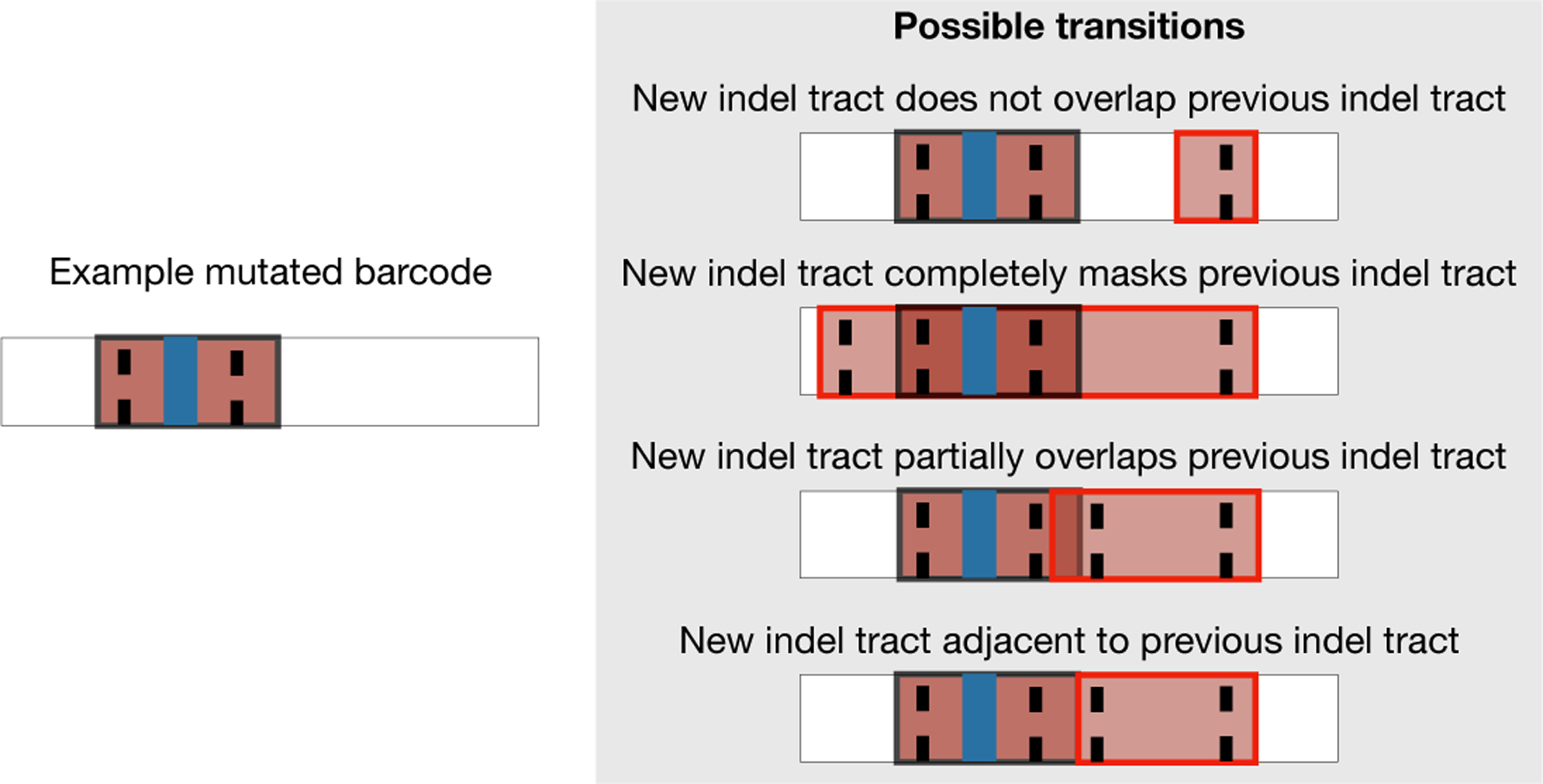
Possible transitions from the left allele are shown on the right. From top to bottom, the mutation process can introduce a new indel tract that does not overlap, completely masks, partially overlaps, or is adjacent to the previous indel tract.

2.1.2. Mutation process.

The mutation process up to time T is formulated as a continuous time Markov chain {X(t) : 0 ≤ t ≤ T } with state space Ω. Since Ω is defined as the set of possible alleles, we have implicitly assumed that indel tracts are introduced instantaneously, i.e. nucleotides are inserted and/or deleted immediately after target(s) are cut.

For tree $\mathbb{T}$, denote the leaves for node N as Leaves(N); use Leaves($\mathbb{T}$) to denote the set of all leaves. Let a_L be the allele observed at leaf node L. For the branch ending with node N, denote its length as t_N and the Markov process along it as {X_N(t) : 0 ≤ t ≤ t_N}. For simplicity, we present the model in the context of a single barcode. If there are multiple barcodes, we assume in this paper that they are sufficiently far apart that they act in an independent and identically distributed (iid) manner.

2.2. Assumptions.

We now formalize the assumptions presented before. Assumption 1 states that for any indel tract that cuts targets j₀ and j₁, its deletions cannot extend past the cut site of neighboring targets j₀ − 1 and j₁ + 1. Note that it can still deactivate neighboring targets by mutating nucleotides at the edge of these targets. We use this assumption to limit the set of possible mutation histories.

Assumption 1. Each indel tract IT[p₀, p₁, s, j₀, j₁] satisfies c(j₀ − 1) < p₀ ≤ c(j₀) and c(j₁) ≤ p₁ < c(j₁ + 1).

To formalize Assumptions 2A-C, define a target tract as a set of indel tracts that cut and deactivate the same target(s). A target tract, denoted $\text{TT}\left[j_0^{\prime },j_0,j_1,j_1^{\prime }\right]\left(j_0^{\prime }\le j_0\le j_1\le j_1^{\prime }\right)$, is the set of all indel tracts that cut targets j₀ and j₁ and delete nucleotides such that targets $j_0^{\prime }$ through $j_1^{\prime }$ are inactive, i.e.

$$\text{TT}\left[j_0^{\prime },j_0,j_1,j_1^{\prime }\right]=\left\{\text{IT}\left[p_0,p_1,s,j_0,j_1\right]:p_0\in \text{pos}\left(j_0^{\prime }\right),p_1\in \text{pos}\left(j_1^{\prime }\right)\right\}.$$ (3)

For instance, TT[2, 2, 3, 4] is the set of indel tracts that cut targets 2 and 3, introduce deletions rightward that deactivate target 4 but not beyond, and introduce short deletions leftward so that target 1 is unaffected. Every indel tract d belongs to a single target tract, which we denote TT(d).

The second assumption states that the instantaneous rate of introducing indel tract d into allele a is the product of the rate of introducing any element from TT(d), which only depends on the target status of a, and the conditional probability of introducing d given TT(d). It also states that the mutation process is irreversible and homogeneous. As such, we treat the GESTALT barcode as a molecular clock. Note that the total mutation rate of a barcode varies over time based on which targets are active, but the model for the transition rates is stationary.

Assumption 2. Let a be an allele, d be an indel tract that can be introduced into a, and τ = TT(d). The instantaneous rate of introducing d in a at time t can be factored into two terms: first, a function that only depends on the triple (τ, TargStat(a), t), and second, the conditional probability of introducing d given τ:

$$\begin{array}{l}q\left(a,\text{Apply}\left(a,d\right)\right):=\underset{\text{Δ}\to 0}{\lim }\frac{\mathrm{Pr}\left(X\left(\text{Δ}\right)=\text{Apply}\left(a,d\right)|X\left(0\right)=a\right)}{\text{Δ}}\\ =h\left(\tau ,\text{TargStat}\left(a\right)\right)\mathrm{Pr}\left(d|\tau \right).\end{array}$$

Moreover, h(τ, TargStat(a)) = 0 if τ cuts a target that is inactive in a.

Using Assumptions 1 and 2, we can calculate the (approximate) likelihood efficiently as described below. Assume the topology is fixed for now, which we denote as $\mathbb{T}$.

2.3. Summing over likely ancestral states.

The first step to calculating the likelihood is to characterize the possible ancestral states. In this section, we provide a recursive algorithm for characterizing a subset of the ancestral states, which should capture all the likely ancestral states and only exclude those with very small probability.

Our approximation of the likelihood excludes mutation histories where overlapping indel tracts merged but did not fully mask one another:

Approximation 1. The probability of indel tracts merging is approximately zero, i.e.

$$\begin{array}{l}\mathrm{Pr}\left(X_{\text{L}}\left(t_{\text{L}}\right)=a_{\text{L}}\forall \text{L}\in \text{Leaves}\left(\mathbb{T}\right)\right)\\ \approx \mathrm{Pr}\left(X_{\text{L}}\left(t_{\text{L}}\right)=a_{\text{L}}\forall \text{L}\in \text{Leaves}\left(\mathbb{T}\right),noindeltractsmerged\right).\end{array}$$ (4)

We will refer to the right-hand probability as the approximate likelihood. We believe merge events are rare since they occur when deletion lengths are long, whereas most deletions are short in McKenna et al. (2016). By excluding merge events, we show that the set of ancestral states in Approximation 1 can be expressed compactly.

Now, let us define a partial ordering among alleles using Approximation 1 and Assumption 1. Given two alleles a, $a^{\prime }\in \text{Ω}$, $a\underset{¯}{\prec }{a}^{\prime }$ means that a can transition to a^′ without merging indel tracts, i.e. there is a sequence of indel tracts ${\left\{d_i\right\}}_{i=1}^m$ for some m ≥ 0 such that

$$a^{\prime }=\text{Apply}\left(d_m,\text{Apply}\left(d_{m-1},\dots \text{Apply}\left(d_1,a\right)\right)\right)$$

where no indel tracts merge. Then, the set of “likely” ancestral states at internal node N in tree $\mathbb{T}$ is defined as

$$\text{AncState}\left(\text{N}\right)=\left\{a\in \text{Ω}:a\underset{¯}{\prec }{a}_{\text{L}}\forall \text{L}\in \text{Leaves}\left(\text{N}\right)\right\}.$$ (5)

(Note that AncState(·) is also defined for leaf nodes, in which case it is the set of alleles that likely preceded the observed allele.) To calculate the approximate likelihood in (4), we marginalize over AncState(N) at each internal node N.

We can characterize AncState(N) using only two building blocks (Fig 4): wildcards and singleton-wildcards. A wildcard² WC[j₀, j₁] is the set of all indel tracts that only deactivate targets within the range j₀ to j₁, inclusive:

$$\text{WC}\left[j_0,j_1\right]=\left\{\text{IT}\left[p_0^{\prime },p_1^{\prime },s^{\prime },j_0^{\prime },j_1^{\prime }\right]:\text{pos}\left(j_0-1\right)<p_0^{\prime },p_1^{\prime }<\text{pos}\left(j_1+1\right)\right\}.$$ (6)

Fig 4:

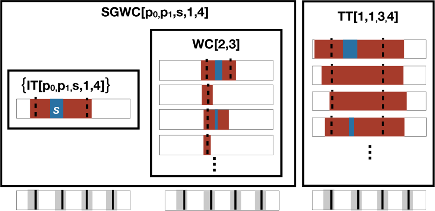
Relationship between indel tracts (IT), target tracts (TT), wildcards (WC), and singleton-wildcards (SGWC). Each IT is shown in the context of a barcode, and the unmodified barcode is shown underneath for reference. Each box represents a set of ITs. For example, the singleton set {IT[p₀, p₁, s, 1, 4]} is the indel tract that cuts targets 1 and 4, deletes positions p₀ to p₁, and inserts sequence s. Wildcard WC[2, 3] contains all indel tracts that only deactivate targets 2 and/or 3. SGWC[p₀, p₁, s, 1, 4] is the union of the singleton set {IT[p₀, p₁, s, 1, 4]} and the internal wildcard WC[2, 3]. TT[1, 1, 3, 4] is the set of indel tracts that cut targets 1 and 3 and deactivate 1 to 4.

A singleton-wildcard SGWC[p₀, p₁, s, j₀, j₁] is the union of the singleton set {IT[p₀, p₁, s, j₀, j₁]} and its inner wildcard WC[j₀ + 1, j₁ − 1], if it exists:

$$\left\{\begin{array}{ll}\left\{\text{IT}\left[p_0,p_1,s,j_0,j_1\right]\cup \text{WC}\left[j_0+1,j_1-1\right]\right\}\hfill & \text{if\hspace{0.17em}}{j}_0+1\le j_1-1\hfill \\ \left\{\text{IT}\left[p_0,p_1,s,j_0,j_1\right]\right\}\hfill & \text{otherwise}.\hfill \end{array}\right.$$ (7)

Two or more wildcards (WCs) and/or singleton-wildcards (SGWCs) are disjoint if the maximum ranges of targets deactivated by indel tracts in these sets do not overlap.

Given a set of indel tracts D, let the alleles generated by D, denoted Alleles(D), be the set of alleles that can be created using subsets of D:

$$\begin{array}{l}\left\{{\left\{\text{IT}\left[p_{0,k},p_{1,k},s_j,j_{0,k},j_{1,k}\right]\right\}}_{k=1}^m\right.\subseteq D:\\ \left.m\in \mathbb{N},p_{1,k}<p_{0,k+1},j_{1,k}<j_{0,k+1}\forall k=1,\dots m-1\right\}.\end{array}$$

Then for leaf L with allele ${\left\{\text{IT}\left[p_{0,k},p_{1,k},s_k,j_{0,k},j_{1,k}\right]\right\}}_{k=1}^m$, AncState(L) is any subset of the alleles generated by its corresponding singleton-wildcards, i.e.

$$\text{AncState}\left(\text{L}\right)=\text{Alleles}\left(\underset{k=1,\dots ,m}{\cup }\text{SGWC}\left[p_{0,k},p_{1,k},s_k,j_{0,k},j_{1,k}\right]\right).$$

We now define a recursive procedure to characterize AncState(·) for all nodes in the tree. We have already established that AncState for a leaf node is characterized by a union of disjoint SGWCs. To recur up the tree, Lemma 1 states that AncState(N) for node N is also characterized by a union of disjoint WC/SGWCs. The proof is given in Section B.

Lemma 1. Consider any internal node N with children nodes C₁, …, C_k. For each child C_K, suppose

$$\text{AncState}\left({\text{C}}_k\right)\subseteq \text{Alleles}\left(\underset{m=1}{\overset{M_{{\text{C}}_k}}{\cup }}{D}_{{\text{C}}_k,m}\right)$$ (8)

Where ${\left\{D_{{\text{C}}_k,m}\right\}}_{m=1}^{M_{{\text{C}}_k}}$ are pairwise disjoint wildcards and/or singleton-wildcards. Then, AncState(N) can be written in the form of (8) where ${\left\{D_{\text{N},m}\right\}}_{m=1}^{M_{\text{N}}}$ are disjoint wildcards and/or singleton-wildcards and is equal to the non-empty intersections of $D_{{\text{C}}_1,m_1}\cap \dots \cap D_{{\text{C}}_K,m_K}$, i.e.

$$\left\{D_{{\text{C}}_1,i_1}\cap \dots \cap D_{{\text{C}}_K,m_K}:m_1=1,\dots ,M_{{\text{C}}_1},\cdots ,m_K=1,\dots ,M_{{\text{C}}_K}\right\}\backslash \cancel{0}.$$ (9)

In practice, we use the recursive algorithm in Section B.2 of the Supplement to compute AncState(·) exactly for additional computational efficiency.

2.4. Lumpability.

The previous section discussed approximating the likelihood by summing over likely ancestral states. Nevertheless, there are still an infinite number of these likely ancestral states. Next, we use Assumption 2 and efficiently compute the approximate likelihood by marginalizing over a small number of “lumped” states.

Lumpability, a well-studied property for Markov chains, states that the behavior of a Markov process can be described by a Markov process over the lumped states (Kemeny et al., 1976; Hillston, 1995) (Fig 5):

Fig 5:

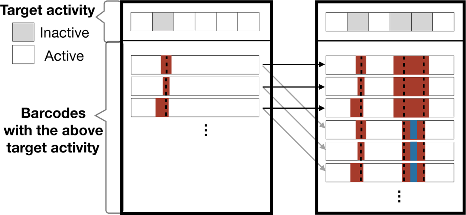
An example of lumping together barcodes that share the same target activity. The two outer boxes correspond to two of the lumped states. The left box is the grouped state for possible ancestral barcode states where the second target is no longer active, while the right box represents when the second, fourth, and fifth targets are no longer active. The arrows represent possible transitions and the color represents the transition rates. Notice that each barcode in the left box has the same set of outgoing arrows. To show that the states are lumpable, we show that the total transition rate out of a barcode in the left box to the right box is identical for all barcodes in the left box.

Definition 1. Let X(t) be a continuous time Markov chain with state space Ω. If there exists a partition {A₁, …, A_M } of Ω and a continuous time Markov chain Y (t) with state space {A₁, …, A_M } such that

$$\mathrm{Pr}\left(X\left(t\right)\in A_i\right)=\mathrm{Pr}\left(Y\left(t\right)=A_i\right)\forall i=1,\dots ,M,$$ (10)

then X is lumpable.

If we can find a partition that satisfies (10), then we can calculate the likelihood over the lumped states instead. The main practical hurdle in using lumpability is finding such a partition (Ganguly, Petrov and Koeppl, 2014).

There is relatively little work on using lumpability in phylogenetics. The one application in Davydov, Robinson-Rechavi and Salamin (2017) calculates the likelihood of a codon model approximately by assuming states are lumpable, even though this is not satisfied. Here we show that lumpability is satisfied exactly in our setting. Since our solution partitions the state space differently at each node, we must extend Felsenstein’s pruning algorithm (Felsenstein et al., 1981) to calculate the approximate likelihood (4).

We will define a partition of Ω at node N denoted {g(b; N) : b ∈ B} for some index set B. We partition the states based on their target status and whether or not they are likely ancestral states (Fig 5), as defined below.

Definition 2. Define index set B to be {0, 1}^M ∪ {other}. For internal tree node N, partition the state space Ω into

$$\left\{\begin{array}{l}g\left(b;\text{N}\right)=\left\{a\in \text{AncState}\left(\text{N}\right):\text{TargStat}\left(a\right)=b\right\}\forall b\in {\left\{0,1\right\}}^M\\ g\left(\text{other};\text{N}\right)=\text{Ω}-\text{AncState}\left(\text{N}\right).\end{array}\right.$$ (11)

For leaf node N, partition the state space Ω into

$$\left\{\begin{array}{l}g\left(b;\text{N}\right)=\left\{a_N\right\}ifb=\text{TargStat}\left(a_{\text{N}}\right)\\ g\left(b;\text{N}\right)=\cancel{0}ifb\in {\left\{0,1\right\}}^{M}andb\ne \text{TargStat}\left(a_{\text{N}}\right)\\ g\left(\text{other};\text{N}\right)=\text{Ω}-\left\{a_{\text{N}}\right\}.\end{array}\right.$$ (12)

Using Assumption 2, we prove in Lemma 4 (see Supplement) that for any b, b^′ ∈ {0, 1}^M, the instantaneous transition rate from any allele a in g(b; N) to g(b^′ ; N) is the same. Therefore we can construct a Markov process over the lumped states {g(b; N) : b ∈ B}, calculate its instantaneous transition rate matrix Q_lump,N as defined in Lemma 4, and exponentiate this matrix to calculate the transition probability

$$\mathrm{Pr}\left(X_{\text{N}}\left(t\right)\in g\left(b^{\prime };\text{N}\right)|X_{\text{N}}\left(0\right)\in g\left(b;\text{N}\right)\right)={\left\{e^{Q_{{\text{lump,N}}^t}}\right\}}_{b,b^{\prime }}\forall b,b^{\prime }\in B.$$ (13)

The following theorem extends Felsenstein’s pruning algorithm to calculate the phylogenetic likelihood by marginalizing over at most 2^M lumped states. For b ∈ B, let the probability of observing the data (marginalizing over likely ancestral states) given that the allele at node N is in partition g(b; N) be denoted

$$p_{\text{N}}\left(b\right)=\mathrm{Pr}\left(X_{\text{L}}\left(t_{\text{L}}\right)=a_{\text{L}}\forall \text{L}\in \text{Leaves}\left(\text{N}\right)|X_{\text{N}}\left(t_{\text{N}}\right)\in g\left(b;\text{N}\right)\right).$$ (14)

Theorem 1. Suppose Assumptions 1 and 2 and Approximation 1 hold. For any internal tree node N, target status b, and nonempty allele group g(b; N), we have

$$p_{\text{N}}\left(b\right)=\prod _{\text{C}\in \text{children}\left(\text{N}\right)}\left\{\sum _{\begin{array}{l}{b}^{\prime }\in {\left\{0,1\right\}}^M\\ g\left(b^{\prime };\text{C}\right)\ne \cancel{0}\end{array}}{p}_{\text{C}}\left(b^{\prime }\right)\mathrm{Pr}\left(X_{\text{C}}\left(t_{\text{C}}\right)\in g\left(b^{\prime };\text{C}\right)|X_{\text{C}}\left(0\right)\in g\left(b;\text{C}\right)\right)\right\}.$$ (15)

where Pr (X_C(t_C) ∈ g(b^′; C)|X_C(0) ∈ g(b; C)) is defined in (13).

The proof for the above theorem is given in Section C.

2.5. Caterpillar trees.

We would like to estimate trees at the finest resolution possible. C-S parsimony produces estimates at a coarse resolution: If the ordering between nodes is ambiguous, they are all grouped under a single parent node. We propose estimating trees by resolving multifurcations at the finer resolution of caterpillar trees (Fig 6a). A caterpillar tree is one where all subtrees branch off of a central path called the spine. We do not assume that the true tree is a caterpillar tree. Rather, we use the caterpillar tree to uncover the order in which indel tracts were introduced.

Fig 6:

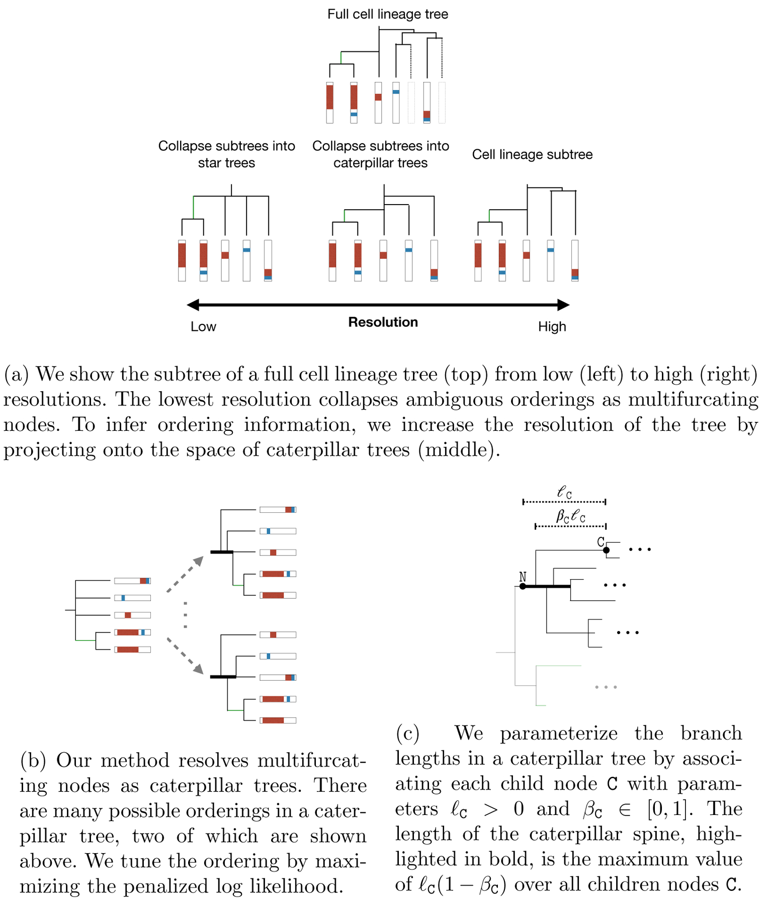
Caterpillar tree goals and parameterization

Calculating the likelihood for all possible branch orderings in a caterpillar tree is computationally intractable because there are K! such orderings for K children nodes. We sidestep this issue by approximating the likelihood using another lower bound: we only marginalize over mutation histories where the alleles are constant along caterpillar spines. To see why this a reasonable approximation, consider the example in Fig 6b. Because the GESTALT mutation process is irreversible, the only possible ancestral state at many internal nodes along the spine is the unmutated barcode. In other words, the allele was constant along most of the spine. Thus, we propose the following approximation of the likelihood.

Approximation 2. We approximate $\mathrm{Pr}\left(X_{\text{L}}\left(t_{\text{L}}\right)=a_{\text{L}}\forall \text{L}\in \text{Leaves}\left(\mathbb{T}\right)\right)$ by considering only the mutation histories that have a constant allele along the caterpillar spines:

$$\mathrm{Pr}\left(X_{\text{L}}\left(t_{\text{L}}\right)=a_{\text{L}}\forall \text{L}\in \text{Leaves}\left(\mathbb{T}\right),allelesareconstantonallspines\right).$$ (16)

This approximation is particularly attractive because it can be computed using the same mathematical expression regardless of the ordering of the children nodes. This allows us to tune the ordering in the caterpillar tree by solving a single continuous optimization problem (Fig 6b).

We re-parameterize the branch lengths for caterpillar branches (Fig 6c). Consider a caterpillar tree with root node N and child node C. Let ℓ_C indicate the distance between C and N. For β_C ∈ (0, 1), let β_Cℓ_C be branch length of C. We can capture all possible orderings for the caterpillar tree rooted at N by varying the values of (ℓ_C, ℓ_C) for each child node C.

With this parameterization, we now extend Theorem 1 to calculate (16). For allele a and node N, define ${\tilde{p}}_{\text{N}}\left(a\right)$ the same as (14) but now assuming both Approximations 1 and 2. Again, apply Felsenstein’s pruning algorithm to recursively compute ${\tilde{p}}_{\text{N}}$ for each node N. However, if N is the root of a caterpillar tree, then ${\tilde{p}}_{\text{N}}\left(a\right)$ is equal to

$$\mathrm{Pr}\left(X_{\text{N}}\left(t_{\text{spine}}\right)=a|X_{\text{N}}\left(0\right)=a\right)\prod _{\text{C}\in \text{children}\left(\text{N}\right)}\left\{\sum _{a^{\prime }\in \text{Ω}}\mathrm{Pr}\left(X_{\text{C}}\left({\mathbf{\ell }}_{\text{C}}/{\beta }_{\text{C}}\right)=a^{\prime }|X_{\text{C}}\left(0\right)=a\right){\tilde{p}}_{\text{C}}\left(a^{\prime }\right)\right\}$$ (17)

where t_spine = max{ℓ_C(1 − β_C) : C ∈ children(N)}. To efficiently calculate the likelihood, we marginalize over the corresponding lumped states instead.

In summary, we have shown how to tune caterpillar trees by solving a single continuous optimization problem. Compared to considering each tree topology separately, this approach is more computationally efficient and performs a more comprehensive search over tree space in practice.

2.6. Model implementation.

We briefly describe our specific model implementation here and leave details to Section E. Each target is associated with a different cut rate λ_j. If targets j₀ and j₁ are active, the rate for cutting target j₀ is λ_j0 and the rate for simultaneously cutting targets j₀ and j₁ is ω(λ_j0 + λ_j1 ) for some ω > 0. We model the distribution of deletion lengths using zero-inflated truncated negative binomial random variables (RVs) and insertion lengths using zero-inflated negative binomial RVs. Finally, Section F.2 discusses our actual code implementation, which includes an additional approximation used to limit memory usage.

3. Estimation method.

Now that the approximate likelihood is computationally tractable, we are ready to estimate the cell lineage tree and mutation model parameters.

3.1. A simple approach.

Consider the following estimation procedure: Given a pool of candidate tree topologies, select the one with the highest likelihood after optimizing over its corresponding parameters. Unfortunately, this procedure can be highly inaccurate for existing GESTALT datasets, where we must estimate thousands of parameters given data generated by a single barcode. Because this problem is high-dimensional, we found in simulations that the maximum likelihood estimate tends to overestimate the length of the leaf branches and the variance of the target rates.

3.2. Penalization.

To improve the estimation accuracy, we propose performing penalized maximum likelihood estimation instead. We penalize large differences in the branch lengths ℓ and target rates λ using

$${\text{Pen}}_{\text{κ}}\left(\theta \right)={\kappa }_1{‖\log \mathbf{\lambda }-\frac{1}{M}\sum _{i=1}^M\log \left({\lambda }_i\right)‖}_2^2+{\kappa }_2{‖\log \mathbf{\ell }-\frac{1}{L}\sum _{i=1}^L\log \left({\mathbf{\ell }}_i\right)‖}_2^2,$$

where κ₁, κ₂ > 0 are penalty parameters and L is dimension of ℓ. A similar branch-length penalty was considered in Kim and Sanderson (2008), but they assume the topology is known.

We cannot directly combine this penalty with the simple approach in Section 3.1 because different topologies may naturally have larger branch length penalties. To ensure that the penalized log likelihood (PLL) is comparable between different topologies, we use an iterative search procedure instead.

For fixed penalty parameters, our estimation procedure follows Algorithm 1. We initialize the topology by selecting a random parsimony-optimal tree from C-S parsimony. At each iteration, we select a random subtree and consider candidate subtree-prune-regraft (SPR) moves that preserve the parsimony score, since parsimony-optimal trees tend to have the highest likelihoods (Fig S7). To make sure the PLLs are comparable, we choose a random leaf from the subtree, calculate the likelihood for the tree from regrafting only this random leaf, and calculate the penalty with respect to the shared subtree (Fig 7).³ We select the SPR move with the highest PLL. In simulations, we found that this procedure progressively improves the tree estimate (Fig S6b). See Section D for a discussion on tuning penalty parameters.

Fig 7:

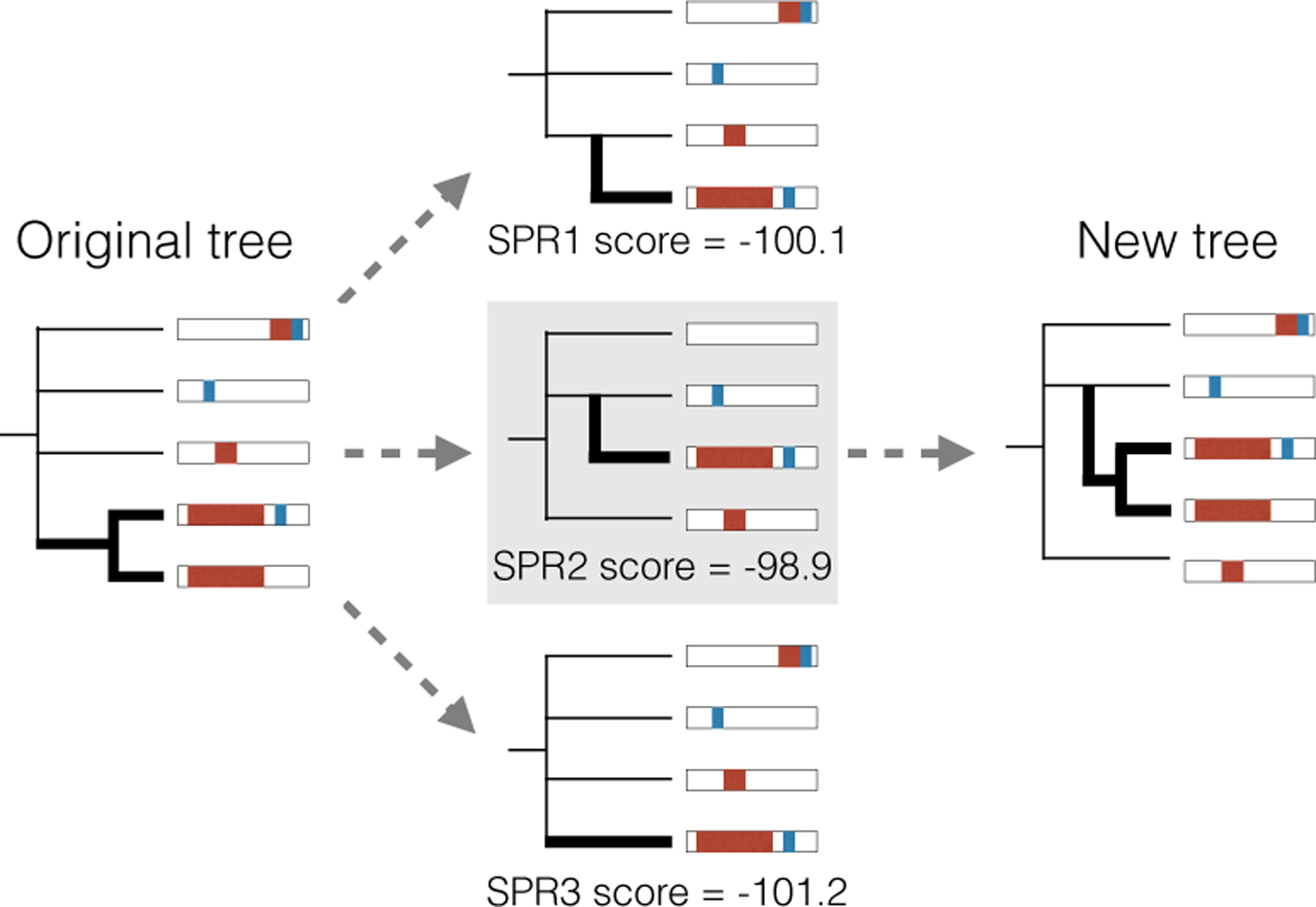
To tune the tree topology, we select a random subtree (left) and score possible SPR moves that preserve the parsimony score by selecting a random subleaf and calculating the maximized penalized log likelihood of the resulting tree (middle). We then update the tree by applying the SPR move with the highest penalized log likelihood (right).

4. Simulation engine and results.

We built a simulation engine of the GESTALT mutation process during embryonic development. Since cell divisions during embryonic development begin in a fast metasynchronous fashion and gradually become more asynchronous (Moody, 1998), the simulation engine generates a cell lineage tree by performing a sequence of synchronous cell divisions followed by a birth-death process where the birth rate decays with time. We mutate the barcode along this cell lineage tree according to our model of the GESTALT mutation process. See Section F for a more detailed description of the simulation setup. The simulation engine generates data that closely resembles the data collected from zebrafish embryos in McKenna et al. (2016) (Fig 8). We can input different barcode designs into the simulation engine to understand how they affect our ability to reconstruct the cell lineage tree.

Fig 8:

Comparison of simulated data (each thin line is a replicate) versus observed alleles from a fish at 4.3 hours post-fertilization (bold line). The distribution of inactive targets and the number of times an allele is observed are similar.

$$\begin{array}{l}\overline{\underset{¯}{\mathbf{Algorithm}\mathbf{1}\text{\hspace{0.17em}Cell\hspace{0.17em}lineage\hspace{0.17em}tree\hspace{0.17em}reconstruction\hspace{0.17em}for\hspace{0.17em}penalty\hspace{0.17em}parameter\hspace{0.17em}κ\hspace{0.17em}\hspace{0.17em}\hspace{0.17em}\hspace{0.17em}\hspace{0.17em}\hspace{0.17em}\hspace{0.17em}\hspace{0.17em}\hspace{0.17em}\hspace{0.17em}\hspace{0.17em}\hspace{0.17em}\hspace{0.17em}\hspace{0.17em}\hspace{0.17em}\hspace{0.17em}\hspace{0.17em}\hspace{0.17em}\hspace{0.17em}\hspace{0.17em}\hspace{0.17em}\hspace{0.17em}\hspace{0.17em}\hspace{0.17em}\hspace{0.17em}\hspace{0.17em}\hspace{0.17em}\hspace{0.17em}\hspace{0.17em}\hspace{0.17em}\hspace{0.17em}\hspace{0.17em}\hspace{0.17em}\hspace{0.17em}\hspace{0.17em}\hspace{0.17em}\hspace{0.17em}\hspace{0.17em}\hspace{0.17em}\hspace{0.17em}\hspace{0.17em}\hspace{0.17em}\hspace{0.17em}\hspace{0.17em}\hspace{0.17em}\hspace{0.17em}\hspace{0.17em}\hspace{0.17em}}}}\\ 1:\text{Initialize\hspace{0.17em}tree\hspace{0.17em}}\mathbb{T}.\text{\hspace{0.17em}Let\hspace{0.17em}the\hspace{0.17em}sequenced\hspace{0.17em}GESTALT\hspace{0.17em}barcodes\hspace{0.17em}be\hspace{0.17em}denoted\hspace{0.17em}}D\text{.}\\ \text{2:\hspace{0.17em}}\mathbf{for}\text{\hspace{0.17em}Iteration }k\mathbf{do}\\ 3:\text{\hspace{1em}Pick a random subtree from }\mathbb{T}\text{. Select one of the leaves C of the subtree.}\\ \text{4:\hspace{1em}}\mathbf{for}\text{\hspace{0.17em}each possible SPR move involving the subtree that doesn’t change the parsimony}\\ \text{\hspace{1em}\hspace{0.33em}\hspace{0.33em}\hspace{0.17em}score }\left(\text{including the no-op}\right)\mathbf{do}\\ 5:\text{\hspace{1em}\hspace{1em}Construct }{\mathbb{T}}^{\prime }\text{ by applying the SPR to leaf C; let }{\mathbb{T}}_{\text{shared}}^{\prime }\text{ be the subtree of }{\mathbb{T}}^{\prime }\text{\hspace{0.17em}when}\\ \text{\hspace{1em}\hspace{1em}\hspace{0.33em}\hspace{0.33em}\hspace{0.33em}excluding\hspace{0.17em}C}\\ \text{6:\hspace{1em}\hspace{1em}Evaluate the penalized log likelihood for the SPR move, maximized with respect}\\ \text{\hspace{1em}\hspace{1em}\hspace{0.33em}\hspace{0.33em}\hspace{0.33em}to parameters }\theta \text{:}\\ \underset{\theta }{\max }\log \underset{\text{Approximation\hspace{0.17em}to\hspace{0.17em}the\hspace{0.17em}likelihood}}{\underbrace{\mathrm{Pr}\left(D,\text{\hspace{0.17em}alleles\hspace{0.17em}are\hspace{0.17em}constant\hspace{0.17em}on\hspace{0.17em}caterpillar\hspace{0.17em}spines,\hspace{0.17em}no\hspace{0.17em}merging\hspace{0.17em}events};{\mathbb{T}}^{\prime },\theta \right)}}\\ -\underset{\text{penalty\hspace{0.17em}on\hspace{0.17em}branch\hspace{0.17em}lengths\hspace{0.17em}and\hspace{0.17em}mutation\hspace{0.17em}parameters}}{\underbrace{{\text{Pen}}_{\text{κ}}\left({\mathbb{T}}_{\text{shared}}^{\prime },\theta \right)}}\\ 7:\mathbf{end}\mathbf{for}\\ 8:\text{\hspace{1em}Update\hspace{0.17em}the tree }\mathbb{T}\text{by performing the SPR move on the subtree with the highest}\\ \text{\hspace{1em}\hspace{0.33em}\hspace{0.33em}\hspace{0.17em}penalized log likelihood}\\ \underset{¯}{\text{9:\hspace{0.17em}}\mathbf{end}\mathbf{for}}\end{array}$$

We used two evaluation metrics to evaluate tree estimates: BHV distance (Billera, Holmes and Vogtmann, 2001) and a new metric we call internal node time correlation. Intuitively, the BHV distance between two trees is the smallest total change in branch lengths to transform one tree into the other (so its minimum value is zero). It is a formal distance metric and therefore enjoys many nice mathematical properties; However, internal node time correlation can be easier to interpret, particularly when BHV distance is large. Given ultrametric trees X and Y for the same set of leaves, the internal node time correlation is calculated as follows (Fig 9):

Fig 9:

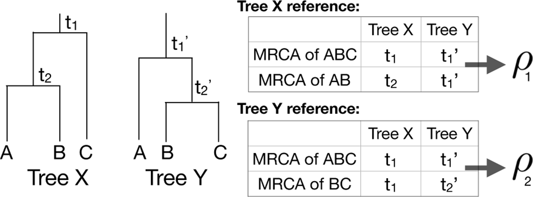
Example calculation of the internal node time correlation. For each tree, calculate the heights for each internal node (e.g. t₁, t₂, $t_1^{\prime }$, $t_2^{\prime }$) and calculate the correlation between the times of the most recent common ancestors (MRCAs) of corresponding leaf groups. The internal node time correlation is the average of correlations ρ₁ and ρ₂.

1. For each internal node in tree X, find the matching node in tree Y that is the most recent common ancestor of the same set of leaves.

2. Calculate the Pearson correlation of the heights of matched nodes.

3. Repeat steps 1 and 2 but swap trees X and Y.

4. Average the two correlation values.

A correlation of 1 means that the trees are exactly the same; the smaller the correlation is, the less similar the trees are.

We compare our method to estimating the tree topology using C-S parsimony (Camin et al., 1965) or neighbor-joining (NJ) (Saitou et al., 1987) and then applying semiparametric rate smoothing (chronos in the R package ape) to estimate node times (Sanderson, 2002). We refer to these approaches as “CS+chronos” and “NJ+chronos,” respectively. Previous in silico analyses measured accuracy in terms of the Robinson-Foulds (R-F) distance, which only evaluates differences in tree topology (Salvador-Martínez et al., 2018). However, this is a very coarse metric and fails to recognize that trees with different topologies can still have very similar internal node times. As such, we also evaluate tree estimates using BHV distance and internal node time correlation; We find that GAPML consistently outperforms the other methods with respect to these two metrics (Fig 10 and Table 1).

Fig 10:

Error of trees estimates from GAPML as well as Camin-Sokal parsimony (CS) and neighbor-joining (NJ) with node time estimation by semiparametric rate smoothing (chronos). Simulated trees has ≈100 leaves, where the barcode is composed of six targets and the number of barcodes is varied from one to six. GAPML outperforms other methods in terms of BHV (left) and the internal node time correlation metrics (middle). The methods are similar in terms of the Robinson-Foulds (RF) metric (right).

Table 1.

Comparison of methods on simulated data using a single barcode with ten targets and around 200 leaves. The 95% confidence intervals are given in parentheses.

Method	BHV	1 - Internal node correlation
GAPML	5.33 (5.06, 5.60)	0.43 (0.39, 0.46)
CS + chronos	6.57 (6.45, 6.9)	0.57 (0.54, 0.60)
NJ + chronos	8.55 (8.51, 8.59)	0.67 (0.66, 0.68)

Figure 10 also shows that GAPML improves in performance as the number of independent barcodes increases. In this simulation, the estimated tree from a single barcode has internal node time correlation of 0.5 with the true tree whereas using six barcodes increases the correlation to 0.9. Even though other analyses have recommended increasing the number of targets in a single barcode to improve tree estimation (Salvador-Martínez et al., 2018), we found that adding independent barcodes is more effective (Fig S5).

Section F.4.1 is a larger simulation study of the method’s asymptotic properties. We show that the method continues to improve, even when there are hundreds of barcodes. Section F.4.2 shows that tree estimates from GAPML are robust to errors resolving ambiguous indels.

5. Real data analysis of a zebrafish – validation.

To validate our method, we reconstructed cell lineages using our method and other tree-building methods on GESTALT data from zebrafish (McKenna et al., 2016). As the true cell lineage tree is not known for zebrafish, we employed indirect measures of validity. For each method, we asked (1) if similar conclusions could be made across different biological replicates and (2) if the tree estimates aligned with the known biology of zebrafish development.

The dataset includes two adult zebrafish where cells were sampled from dissected organs. The organs were chosen to represent all germ layers: the brain and both eyes (ectodermal), the intestinal bulb and posterior intestine (endodermal), the heart and blood (mesodermal), and the gills (neural crest, with contributions from other germ layers). The heart was further divided into four samples— a piece of heart tissue, dissociated unsorted cells (DHCs), FACS-sorted GFP+ cardiomyocytes, and non-cardiomyocyte heart cells (NCs). In addition, datasets were collected from embryos at the dome stage (4.3 hours post-fertilization (hpf)), pharyngula stage (30 hpf), and from early larvae (72 hpf), where the cell types are unknown. We set the total height of each tree estimate to T = 1.

5.1. Replication of developmental relationships between tissue types.

Here, we check if the estimated developmental relationships between tissue types is replicated in the two adult fish samples. For each estimated tree, we calculated the distance between tissues, which we define as the average tree distance between a leaf of one tissue to the closest internal node leading to a leaf from the other tissue, weighted by the allele abundance (Fig 11). (All alleles that were found in the blood were removed since blood is found in all dissected organs and can confound the relationship between organs McKenna et al. (2016).) Recall that all of the fitting procedures are completely agnostic to any tissue source or cell abundance information. We tested if the correlations were significant by permuting the cell types and abundances in the estimated trees. The correlation was 0.730 (p < 0.001) using our method, whereas ‘CS+chronos’ and ‘NJ+chronos’ had correlations of 0.306 (p = 0.21) and −0.325 (p = 0.22), respectively.⁴

Fig 11:

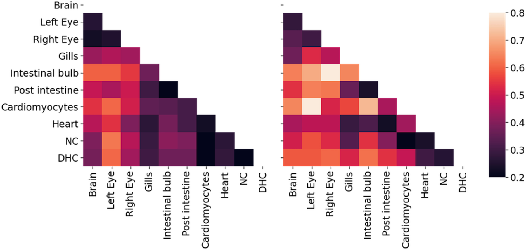
Average distance between tissue sources from adult fish 1 (left) and 2 (right) for tree estimates from GAPML. The distance between tissues is the average time from a leaf of one tissue to the closest internal node with a descendant of the other tissue. The shading reflects distance, where bright means far and dark means close. The tissue distances share similar trends between the two fish. For example, the top (brain and eyes) and lower right (heart-related organs) tend to be the darker regions in both distance matrices.

5.2. Replication of mutation parameters.

Here, we check if the mutation parameters replicate across fish samples. For each time point, the fish replicates were traced using the same GESTALT barcode and processed using the same experimental protocol (Table 2). We compared the estimated target rates from our method to those estimated using a model-free empirical average approach where the estimated target cut rate is the proportion of times a cut was observed in that target in the set of unique observed indels. The average correlation between the estimated target rates from our method were much higher than that for the alternate approach (Table 2). In fact, we can also compare target cut rates between fish of different ages that share the same barcode, even if the experimental protocols are slightly different. The 4.3hpf and 72hpf fish share the same barcode version, and we find that the target rate estimates are indeed similar (Fig 12).

Table 2.

Mean Spearman correlation between the estimated target lambda rates across fish replicates (hpf is short for hours post fertilization). 95% confidence intervals via bootstrap are shown in parentheses. The correlation is higher for GAPML estimates, compared to setting rate estimates as the proportion of times each target was cut.

Fish age	n	Barcode version	GAPML Correlation	Empirical average correlation
4 months	2	7	0.891	0.685
72 hpf	6	7	0.897 (0.855, 0.973)	0.648 (0.616, 0.842)
30 hpf	4	6	0.287(0.287, 0.788)	0.052 (0.052, 0.727)
4.3 hpf	5	7	0.942 (0.942, 0.976)	0.749 (0.714, 0.918)

Fig 12:

Fitted target lambda rates for fish sampled at different time points; Each line corresponds to estimates for a single fish. Fish sampled at 4.3hpf (left) and 72 hpf (middle) used the same barcode and have similar rate estimates. The 30hpf fish (right) used a different barcode and has different rate estimates.

5.3. Recovery of cell-type and germ-layer restriction.

It is well known that cells are pluripotent initially and specialize during development. To evaluate recovery of specialization by tissue type, we calculated the correlation between the estimated time of internal tree nodes and the number of descendant tissue types; to evaluate recovery of specialization by germ layer, we calculated the correlation between the estimated time of internal nodes and the number of germ layers represented at the leaves. (As before, all the estimation methods do not use the tissue origin and germ layer labels.) Since any tree should generally show a trend where parent nodes tend to have more descendant cell types than their children, we compared our tree estimate to the same tree but with random branch length assignments and randomly permuted tissue types. Our method estimated much higher correlations compared to these random trees (Table 3). We show an example of the node times versus the number of descendant cell types and germ layers in Figure 13. The other methods have lower correlation compared to GAPML in all cases, except for ‘NJ + chronos’ in the second adult fish. However, upon inspection, the correlation is high for ‘NJ + chronos’ because it estimates that cells are pluripotent for over 90% of the fish’s life cycle and specialize during a small time slice at the very end.

Table 3.

Correlations between the number of descendant cell types/germ layers vs. the time of internal nodes for different estimation methods. For each tree estimate, we create random trees by fixing the topology but shuffling cell types and assigning random branch lengths. The correlation for these random trees are shown. The p-value is calculated with respect to these random trees.

Adult	Estimation	# tissue types vs time			# germ layers vs time
Fish	Method	Corr	Random corr	p-value	Corr	Random corr	p-value
1	GAPML	−0.476	−0.176	< 0.001	−0.404	−0.125	< 0.001
	CS+chronos	−0.182	0.037	0.002	−0.142	0.032	0.044
	NJ+chronos	−0.271	−0.126	0.003	−0.179	−0.094	0.084
2	GAPML	−0.547	−0.243	<0.001	−0.437	−0.184	0.002
	CS+chronos	−0.389	0.070	0.001	−0.397	0.090	< 0.001
	NJ+chronos	−0.621	−0.236	<0.001	−0.475	−0.183	0.001

Fig 13:

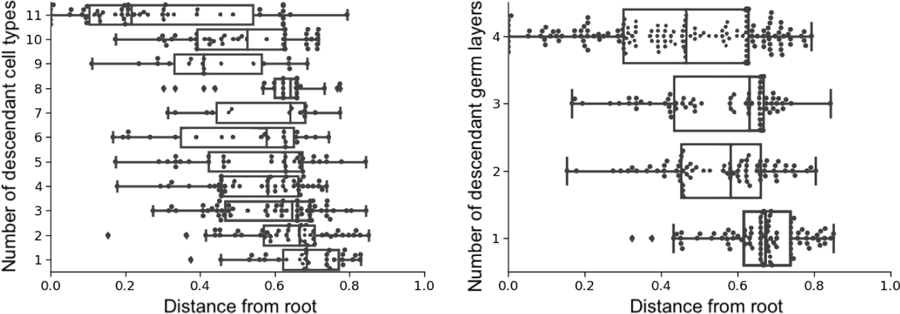
Visualization of internal node times for the first adult fish using GAPML, stratified by the number of descendant cell types (left) and germ layers (right). The estimated node times recover the known phenomenon of cell type and germ layer restriction during organism development.

5.4. Analysis of the zebrafish GESTALT data.

Now we analyze the fitted trees of the adult zebrafish in more detail to check if summaries concord with known zebrafish biology; and generate new hypotheses about zebrafish development and the experimental procedure.

The estimated tissue distance matrices (Fig 11) present a coarse summary of the developmental process. We observe that they recapitulate some well-established facts about zebrafish development. For example, we estimate that tissue types from the endoderm and mesoderm tended to be closer. This signal potentially captures the migration of the endoderm and mesoderm through the blastopore, isolating them from the ectoderm (Solnica-Krezel, 2005). In addition, previous studies established that gills form when the anterior part of the intestine grows toward and fuses with the body integument (Shadrin and Ozernyuk, 2002). Likewise, our method estimates that gill cells are closer to tissues from the endoderm and mesoderm.

Fig 11 also shows that the GFP+ cardiomyocytes tend to be farthest away from other tissue types, which could be either a developmental signal or an artifact of the experimental protocol. GFP+ cardiomyocytes were sorted using fluorescence-activated cell and this purity could drive their separation from the other more heterogeneous organ populations. An interesting biological speculation would be that the myocardial cells are one of the first cells to differentiate during vertebrate embryo development, which could be driving this observed signal (Keegan, Meyer and Yelon, 2004).

The cell lineage tree estimated using GAPML provides significantly more detail than the C-S parsimony tree inferred in McKenna et al. (2016) (Fig 14). Unlike the C-S tree, the GAPML tree infers relative timing of events across parallel subtrees and infers the order of events.

Fig 14:

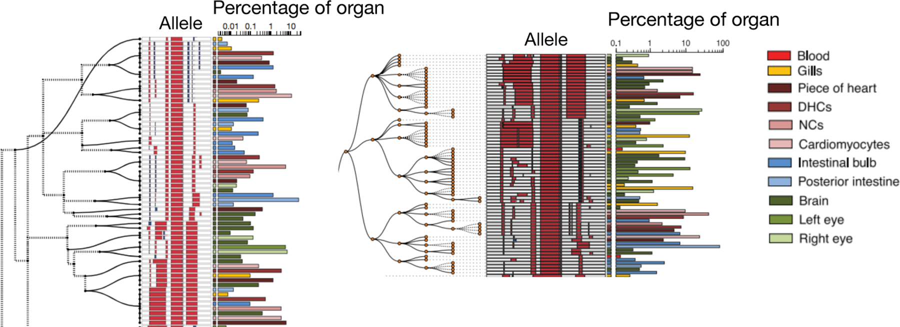
Subtree from trees estimated using GAPML (left) and Camin-Sokal parsimony (right). Red and blue bars in the allele indicate deletions and insertions, respectively. Alleles observed in multiple organs are plotted on separate lines per organ. The barchart on the right of each subfigure indicates the proportion of cells in that organ represented by each allele. The dashed lines in the GAPML tree correspond to the caterpillar spines.

The full tree estimated using GAPML for the first adult zebrafish is displayed in Figure S10. The raw tree data and tools for visualizing the tree are available at https://github.com/matsengrp/gapml. Its longest caterpillar spine starts from the root node and connects all the major subtrees that share no indel tracts. As the zebrafish embryo rapidly divides from the single-cell stage, these initial CRISPR editing events establish the founding cell in each subtree. We see that the last three subtrees at the end of this spine (farthest away from the root) were observed primarily in the intestinal bulb and the posterior intestine. This concords with our understanding of zebrafish development: of the dissected organs, the digestive tract is the last to fully differentiate (Moody et al., 1998). These examples show that this more refined lineage tree can inspire new and interesting biological questions and provide a means to answer them.

5.5. Analysis of mutation parameters.

Finally, our estimated mutation parameters (Table S2) can guide redesigns of the GESTALT barcode. For example, we estimate that Targets 1 and 9 in the barcode from McKenna et al. (2016) have the highest cut rates. To decrease the frequency of intertarget deletions, one suggestion is therefore to move those targets to the center of the barcode and targets with lower cut rates to the outside.

6. Discussion.

We have proposed a statistical model for the mutation process of GESTALT, a lineage-tracing technology that leverages a synthetic barcode of CRISPR/Cas9 targets to record development. Our method, GAPML, estimates the cell lineage tree and the mutation parameters of this system. GAPML outperforms existing methods on simulated data, provides more consistent results across biological replicates, and outputs trees that better concord with our understanding of developmental biology. Its performance will continue to improve with our ability to integrate more barcodes.

Our method provides a number of technical contributions to the phylogenetics literature. Because the GESTALT mutation process violates many of the classical phylogenetic assumptions, we have introduced new assumptions and methods to make the problem computationally tractable. We believe these techniques could be useful for other phylogenetic problems where the common assumptions do not hold.

A limitation of our method is that it treats the barcode as a molecular clock, even though its mutation rates can actually vary due to cell state, e.g. chromatin state and transcriptional activity. Future work includes relaxing the molecular clock assumption, as well as quantifying the uncertainty of our estimates and merging data across sample replicates.

Finally, our methods may be useful for analyzing other CRISPR-based cell lineage tracing technologies. GAPML is most readily applied to techniques that insert arrays of Cas9 targets (Schmidt et al., 2017; Salvador-Martínez et al., 2018) or those that mutate transgenes in organisms (Spanjaard et al., 2018; Alemany, Florescu and Baron et al., 2018). More work needs to be done to adapt it to homing CRISPR guide RNA systems (Kalhor, Mali and Church, 2017; Kalhor, Kalhor and Mejia et al., 2018).