Model-free prediction test with application to genomics data

Significance

Statistical theory has mostly focused on testing the dependence between covariates and response under parametric or semiparametric models. In reality, the model assumptions might be too restrictive to be satisfied, and it is of substantial interest to test the significance of the prediction in a completely model-free setting. Our proposed method is nonparametric and can be applied to a wide range of real applications. It can borrow the strength of the most powerful machine learning regression algorithms and is computationally efficient. We apply the inference approach to the recent cellular indexing of transcriptomes and epitopes by sequencing data and spatially resolved transcriptomics data. The proposed method is more powerful and can produce biologically meaningful results.

Abstract

Testing the significance of predictors in a regression model is one of the most important topics in statistics. This problem is especially difficult without any parametric assumptions on the data. This paper aims to test the null hypothesis that given confounding variables Z, X does not significantly contribute to the prediction of Y under the model-free setting, where X and Z are possibly high dimensional. We propose a general framework that first fits nonparametric machine learning regression algorithms on $Y|Z$ and $Y|(X,Z)$, then compares the prediction power of the two models. The proposed method allows us to leverage the strength of the most powerful regression algorithms developed in the modern machine learning community. The P value for the test can be easily obtained by permutation. In simulations, we find that the proposed method is more powerful compared to existing methods. The proposed method allows us to draw biologically meaningful conclusions from two gene expression data analyses without strong distributional assumptions: 1) testing the prediction power of sequencing RNA for the proteins in cellular indexing of transcriptomes and epitopes by sequencing data and 2) identification of spatially variable genes in spatially resolved transcriptomics data.

With the advancement of technology, scientists can collect massive datasets that contain covariates of interest X, confounding variables Z, and response Y. X and Z are often high dimensional. A central theme of statistics is to provide modeling and testing tools for the relationship between X and Y. Traditional statistical theories usually consider parametric models on the data, for example, assuming $Y|(X,Z)$ follows a normal distribution or $\mathbb{E}(Y|X,Z)$ follows a linear model. The modern machine learning community has developed powerful predictive models without parametric assumptions. However, a critical gap remains in the literature: in the model-free setting, how to test whether a set of features have significant predictive power on a response variable. Specifically, we are interested in testing

$$\begin{array}{l}{H}_0:\mathbb{E}(Y|Z)=\mathbb{E}(Y|X,Z)\hspace{1em}\text{vs}.\\ H_1:\mathbb{E}(Y|Z)\ne \mathbb{E}(Y|X,Z).\end{array}$$ [1]

The null hypothesis implies that the regression function $E[Y|Z=z]=E[Y|X=x,Z=z]$ at every point (x, z). When only X is included in the model, the problem of interest becomes

$$H_0:\mathbb{E}(Y)=\mathbb{E}(Y|X)\hspace{1em}\text{vs}.\hspace{1em}{H}_1:\mathbb{E}(Y)\ne \mathbb{E}(Y\text{|}X).$$ [2]

Under the linear model or the single (multiple) index models, the testing problems [1] and [2] are equivalent to testing whether the coefficient of X is equal to zero. From the view of variable selection, [1] and [2] aim at testing whether X is relevant in the prediction of Y. Even though the past decades have witnessed many contributions to the statistics literature on variable selection (1), it is still extremely challenging to test hypotheses [1] and [2] without parametric or structural assumptions on X and Y.

The key idea of our method is to compare whether a powerful machine learning algorithm, fitted with X included as part of the input, performs significantly better than without X. The method begins by splitting the data into two subsets: D₁ and D₂. We first fit two machine learning regression algorithms on D₁: one with X and the other without X. Then, we compare the performance of the two fitted models on D₂ by calculating the difference between the two means of residual squares. The goal is to detect any potential incremental predictive power for Y provided by X by differentiating the performance of the two models. Under H₀, the two models perform similarly to each other, and the residuals should also have similar values. Under H₁, the fitted machine learning algorithm should produce a smaller residual compared to the null model. The test statistic has a limiting normal distribution, and the P value can be computed efficiently.

The first application of the proposed method is in cellular indexing of transcriptomes and epitopes by sequencing (CITE-seq) data, where surface protein and sequencing RNA are measured simultaneously at the single-cell level. CITE-seq data are a type of single-cell multimodal omics data, a research area labeled “Method of the Year 2019” by Nature Methods. While gene expression data have been extensively studied in the single-cell literature, the prediction of surface proteins based on RNA sequencing (RNA-seq) has only been studied in recent literature (2). The imputation of proteins is of great interest because the proteins are functionally involved in cell signaling and cell–cell interactions (3). Due to the importance of CITE-seq data in scientific discoveries of human biology, scientists implemented various tools for studying the relationship between proteins and RNA gene expression (4, 5). For example, Stuart et al. (6) and Hao et al. (4) used k-nearest neighbors to predict protein levels. Zhou et al. (2) implemented deep neural networks to impute surface proteins based on gene expression. Our method can be used to verify whether such models have nontrivial predictive accuracy via a statistically principled test.

The other application arises in spatial transcriptomics data. Scientists have collected high-throughput transcriptome profiling that contains the spatial location of genetic measurements and aim to find the genes that are variable across the tissue. This topic has inspired great interest, and Nature Methods recently selected spatially resolved transcriptomics as “Method of the Year 2020” (7). Gene expression and the spatial location play the roles of Y and X, respectively. Existing literature on spatially variable gene (SVG) detection can be roughly classified into two categories. The first category assumes a parametric model for the distribution of $Y|X$. For example, the gene expression profiles Y were assumed to follow a normal distribution in ref. 8, given X and other spatial structures. The spatial correlation in ref. 9 is also derived under the normal distribution theory. Because gene expression is usually count data, the other way is to assume Y follows a Poisson distribution with rate parameter depending on the spatial correlations among spots (10). The second approach does not assume a parametric model. Some methods utilize certain metrics that measure the spatial distribution within a local radius constraint (11, 12). This method tends to be sensitive to the choice of the local regions in the tissue. Another approach is to test the independence of gene expression and spatial location (13). In comparison, our test specifically targets the expectation of gene expression and provides great flexibility and interpretative results for the data. We illustrate the details in the numerical analysis.

Methods

Sample Splitting and Regression.

Suppose we observe data $(X_1,Z_1,Y_1),\hspace{0.17em}\dots ,\hspace{0.17em}(X_n,Z_n,Y_n)$ independently from the joint distribution of (X, Z, Y). We begin by splitting the index set $\mathcal{I}=\{1,\dots ,n\}$ into two subsets, ${\mathcal{I}}_1=\{1,2,\dots ,n_1\}$ and ${\mathcal{I}}_2=\{n_1+1,\dots ,n\}$. Denote $n_2≔n-n_1$. Let $D_1=\{(X_i,Y_i),i\in {\mathcal{I}}_1\}$ and $D_2=\{(X_i,Y_i),i\in {\mathcal{I}}_2\}$ be the two subsets of the data.

The key feature of our method is that it does not rely on a parametric model of $\mathbb{E}(Y|X,Z)$ and can easily adapt to different data types or even high-dimensional data. Specifically, we assume the most general form of regression model

$$Y=g(X,Z)+\epsilon ,$$

where ε satisfies $\mathbb{E}(\epsilon |X,Z)=0$. Our method begins with fitting a flexible machine learning algorithm for $\mathbb{E}(Y|X,Z)$ by optimizing

$${\mathcal{L}}_{n_1}(Y,g(X,Z))+{\mathcal{P}}_{\lambda }(g)$$ [3]

over a function class $\mathcal{G}$ and denoting the estimated regression function as ${\widehat{g}}_1$. Here ${\mathcal{L}}_{n_1}(·,·)$ is an empirical loss function. When Y is continuous, we can choose the least square loss function. We may use the Huber loss when Y has a heavy tail. When Y is discrete, we can use the hinge loss or cross-entropy loss functions. The regularization term ${\mathcal{P}}_{\lambda }$ controls the complexity of the estimated model. It is especially useful to let ${\mathcal{P}}_{\lambda }$ be the L₁ regularization when the covariates X is of high dimension. We also train the model without X by optimizing

$${\mathcal{L}}_{n_1}(Y,g(Z))+{\mathcal{P}}_{\lambda }(g)$$ [4]

and denote the estimated regression function as ${\widehat{g}}_0$.

To ensure the validity of the test, we train ${\widehat{g}}_0$ and ${\widehat{g}}_1$ based on the first subset of the data D₁. ${\widehat{g}}_0$ and ${\widehat{g}}_1$ can be fitted using any algorithms, including neural networks, SVM, or random forest. Under H₀, ${\widehat{g}}_1$ should not perform better than ${\widehat{g}}_0$ since X does not contribute to the prediction of Y, while under H₁, a good machine learning regression algorithm ${\widehat{g}}_1$ should pick up the information from X and result in smaller residuals compared to the null model. This intuition motivates us to implement a two-sample test to compare the squared residuals between ${\widehat{g}}_0$ and ${\widehat{g}}_1$ when performing prediction based on D₂.

Two-Sample Comparison.

To evaluate the performance of ${\widehat{g}}_0$ and ${\widehat{g}}_1$, we perform two-sample comparisons on the fitted residuals of the two models based on the data in D₂. The most natural approach is the two-sample t test (TS). Define

$$T_{TS}=\frac{1}{n_2}{\displaystyle \sum _{i\in {\mathcal{I}}_2}\left[{\left\{Y_i-{\widehat{g}}_1(X_i,Z_i)\right\}}^2-{(Y_i-{\widehat{g}}_0(Z_i))}^2\right]}.$$

The test will reject H₀ if T_TS takes a large negative value. The test compares the mean square errors (MSE) of two models, under the assumption of the existence of the second-order moments of the data. The comparison of MSE is natural because $E(Y|Z)$ is the optimal predictor of Y (when only considering Z) in the MSE sense:

$$E\left\{{[Y-r(Z)]}^2\right\}\ge E\left\{{[Y-E(Y|Z)]}^2\right\}\hspace{1em} \text{for} \text{all} r(·)\in {\mathcal{L}}_2.$$

See, for example, theorem 2.1 ref. 14. To give some intuition about the validity of such a test, consider the simpler case where only X is included in the model, and the squared loss function is used. In this case, ${\widehat{g}}_0(Z_i)$ is equivalent to the sample mean of Y in D₁, which we write as $\widehat{\mu }$.

Under H₀, X does not contain predictive information about Y so that $\mathbb{E}(Y|X)=\mathbb{E}(Y)$ and ${\widehat{g}}_1$ performs no better than $\widehat{\mu }$, and T tends to be nonnegative, regardless of the choice of ${\widehat{g}}_1$. Under H₁, ${\widehat{g}}_1(X)$ aims to approximate $\mathbb{E}(Y|X)$, and the positive component in T_TS has a large sample limit of $\mathbb{E}{(Y-{\widehat{g}}_1(X))}^2=\mathbb{E}[{(Y-\mathbb{E}(Y|X))}^2]+\mathbb{E}[{({\widehat{g}}_1(X)-\mathbb{E}(Y|X))}^2]=\mathbb{E}[\text{Var}(Y|X)]+\text{MSE}({\widehat{g}}_1)$. On the other hand, the large sample limit of the negative component in T_TS is $\text{Var}(Y)=\mathbb{E}[\text{Var}(Y|X)]+\text{Var}[\mathbb{E}(Y|X)]$. Therefore, when $\text{MSE}({\widehat{g}}_1)<\text{Var}[\mathbb{E}(Y|X)]$, the test statistic T_TS will be negative, and the test will have nontrivial power.

To summarize, the test that rejects large negative values of T_TS satisfies the following properties.

• 1)Under H₀, the false positive is always controlled regardless of the choice of ${\widehat{g}}_1$.
• 2)Under H₁, the test has good power as long as $\text{MSE}({\widehat{g}}_1)<\text{Var}[E(Y|X)]$.

Our split-fit-test framework allows us to use other forms of two-sample comparisons. For example, in certain scenarios, we may want to use the rank-sum test (RS):

$$T_{RS}=\frac{1}{n_2^2}{\displaystyle \sum _{i,j\in {\mathcal{I}}_2}\mathbb{I}}\left(|Y_i-{\widehat{g}}_1(X_i,Z_i)|<|Y_j-{\widehat{g}}_0(Z_j)|\right)-\frac{1}{2}.$$

Due to the use of the indicator function, the rank-sum test performs well for data with heavy-tailed distributions or outliers. The intuition behind this test is that when X is informative about Y, the fitted residuals $Y_i-{\widehat{g}}_1(X_i,Z_i)$ will likely be smaller than those from the null model.

We briefly discuss the pros and cons of the two tests. The rank-sum test, as later shown in the numerical studies, is very robust when the response variable Y has a heavy-tailed distribution but may have an inflated type I error if the noise is highly skewed as the quantiles are no longer aligned with expectation. Therefore, we recommend using the rank-sum comparison only if the exploratory analysis does not suggest a highly skewed noise distribution.

In this paper, we obtain the P value using permutation. The algorithm is summarized as follows.

• 1.For $i\in {\mathcal{I}}_2$, calculate $U_i=Y_i-{\widehat{g}}_1(X_i,Z_i)$ and $V_i=Y_i-{\widehat{g}}_0(Z_i)$. Let $\mathcal{S}=\{U_i,i\in {\mathcal{I}}_2\}\cup \{V_i,i\in {\mathcal{I}}_2\}$.
• 2.Calculate the test statistic T based on U_i and V_i, $i\in {\mathcal{I}}_2$.
• 3.For $b=1,\dots ,B$,
  • (a)Obtain sample $\{U_i^{*},i\in {\mathcal{I}}_2\},\hspace{0.17em}\{V_i^{*},i\in {\mathcal{I}}_2\}$ by randomly partitioning $\mathcal{S}$ into two equal-sized subsets.
  • (c)Calculate $T_b^{*}$ using $U_i^{*}$ and $V_i^{*},\hspace{0.17em}i\in {\mathcal{I}}_2$.
• 4.Calculate P value: $B^{-1}{\displaystyle {\sum }_{b=1}^B\mathbb{I}}\{T>T_b^{*}\}$.

In this paper, we used equal random split and let n₁ = n₂. When the sample size is too small, a V-fold cross-validation type unequal split can also be applied, such as the V-fold algorithm proposed in ref. 15. Under suitable conditions, one can show that the test statistic used in the above two-sample residual comparison has a Gaussian asymptotic null distribution. For example, the asymptotic Gaussianity of the t statistic T_TS has been established in ref. 15. The asymptotic theory for the rank-sum test can be derived using a similar strategy as in ref. 16. As a result, the last step of the P value calculation can be modified by first estimating the SD of $\{T_b^{*},b=1,\dots ,B\}$, denoted as ${\widehat{\sigma }}_B$, and then calculating the P value as ${\mathrm{\Phi }}^{-1}(T/{\widehat{\sigma }}_B)$, where ${\mathrm{\Phi }}^{-1}$ is the cumulative distribution function of standard normal distribution. This will provide a P value with relatively high resolution.

Combine Multiple Splits.

The method described so far is based on a single random split of the data. In practice, multiple splits could be used to mitigate the additional randomness introduced by the sample split. To combine the dependent P values obtained from multiple splits, we use the Cauchy combination test proposed in ref. 17. The idea is to first transform the P value of each test into a standard Cauchy distribution, then compute the average of the transformed values and compare it with a standard Cauchy’s tail behavior. Specifically, assume we perform B splits and obtain P values $p_1,\dots ,p_B$. Let T₀ be defined by

$$T_0=\frac{1}{B}{\displaystyle \sum _{j=1}^B\tan }\{(0.5-p_i)\pi \}.$$

The P value of the combined test can be approximated by

$$\text{p-value}=0.5-\{\arctan (T_0)\}/\pi .$$

In our numerical studies, we combine the results of 5 to 15 random splits depending on the varying computation cost in different datasets. It turns out that the type I error of the combined test can be controlled very well, and its power exceeds those of single splits.

For notation simplicity, we name the single-split regression-based rank-sum test as RS-S and its multiple version as RS-M. Correspondingly, we name the single-split regression-based t test as TT-S and its multiple version as TT-M.

Test Predictability of Proteins in CITE-seq Data

Background.

CITE-seq is a recent multimodal single-cell phenotyping technology (6). The dataset contains measurements of single-cell gene expression and surface proteins. Researchers are familiar with gene expression data, which are high-dimensional, noisy, and sparse. By contrast, surface protein data are low-dimensional, highly informative, but more expensive to measure. Thus, it is of great interest to predict protein measurements based on gene expression (2, 4–6). These prediction models provide a better understanding of the translation from RNA-seq to proteins and also enable researchers to predict the proteins when only the RNA sequence is measured at the single-cell level.

We use the human peripheral blood mononuclear cell (PBMC) CITE-seq data, which have been analyzed in ref. 4, as our primary example. While different types of cells usually contain different patterns of gene expression and proteins, it is unclear how the predictability of proteins varies across cell types. In this section, we investigate the predictability of protein expression in different types of human blood immune cells.

Simulations.

To verify the performance of the proposed method, we perform simulations for the predictive tests based on rank-sum test and two-sample t test. We consider both single-split and multiple-split data and set the split times in multiple-split data to be 10. XGBoost tree (18) is implemented as the regression algorithm due to its fast computational speed and good flexibility to capture nonlinear relationships. We also compare the performance of XGBoost with linear regression in SI Appendix, Fig. S4 to demonstrate its superior performance. We compare our method with the Martingale difference correlation (MDC), which has a similar goal of testing mean independence and was proposed by Shao and Zhang in ref. 19.

To demonstrate the performance for high-dimensional, sparse signal and heavy-tail noise, we generate the response Y_i as the function of the first element of the covariates $X_{i,1}$ with a heavy-tail distributed error term. Specifically, let

$$Y_i=a\times f(X_{i,1})+{\epsilon }_i,\hspace{1em}{\epsilon }_i\sim \text{Cauchy}(0,1).$$

a is used to control the signal level. a = 0 implies that H₀ is true, and a > 0 represent H₁ holds. The details of $f(·)$ in each model are given in SI Appendix.

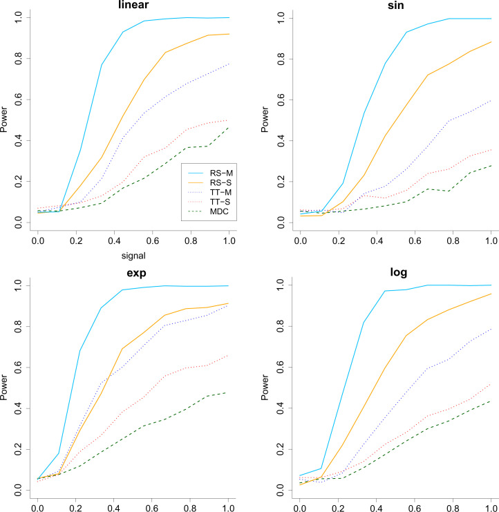
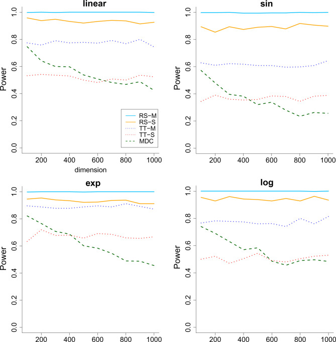
We consider two simulation scenarios: 1) the signal level a increases from 0 to 1 when the sample size and dimension are fixed to be 200 and 1,000 and 2) the dimension of X increases from 100 to 1,000 when keeping the sample size and a fixed. Each simulation is repeated 1,000 times, and we report the average power in Figs. 1 and 2, where the type I error is controlled at $\alpha =0.05$. As we can see, all methods have a valid type I error rate. The multiple-split rank-sum test performs the best in terms of power, followed by the single-split rank-sum test. The two-sample t test seems to be unsuitable for the heavy-tailed data. As for MDC, we see that it not only is unsuitable for heavy-tailed data but also suffers from the curse of dimensionality when the covariates are high-dimensional. This demonstrates the advantage of the proposed methods.

Fig. 1.

The power (vertical) versus signal (horizontal) for the all the methods when the response has heavy-tailed distribution and $\alpha =0.05$. The RS stands for rank-sum test, and TT stands for two-sample t test. M means multiple split, and S represents a single split. Across the 4 panels, the relationship between Y and the first covariate is linear, sine (sin), exponential (exp) and logarithmic (log).

Fig. 2.

The power (vertical) versus dimension (horizontal) for the all the methods when the response has heavy-tailed distribution and the dimension of the covariates increases. $\alpha =0.05$. The RS stands for rank-sum test and TT stands for two-sample t test. M means multiple split, and S represents single split. Across the 4 panels, the relationship between Y and the first covariate is linear, sine (sin), exponential (exp) and logarithmic (log).

Human PBMC Data.

After applying standard quality control procedures (4), the human PBMC data contain 20,729 gene expressions and 228 proteins measured on 161,764 cells. After removing the two proteins (CD26-1 and TSLPR) that contain mostly zeros, we obtain 226 proteins in total. According to the cell annotations, we can classify all the cells into eight different types. Following the standard convention in single-cell analysis, we restrict our analysis to the top 5,000 highly variable gene sets. The marker genes for each cell type are obtained by implementing the FindMarkers function from Seurat (4). The number of cells and marker genes of each type are summarized in Table 1. The total number of marker genes is less than the sum of individual cell types because different cell types may share the same marker genes. Under the testing framework of [1] and [2], we are mainly interested in two questions:

Table 1.

Number of cells and marker genes in each cell type in the human PBMC data

Cell type	Cells	Marker genes
Mono	49,010	1,007
CD4 T	41,001	576
CD8 T	25,469	313
NK	18,664	519
B	13,800	598
Other T	6,789	122
DC	3,589	372
Other	3,442	273
Total	161,764	1,692

• 1)Do marker genes in different cell types (defined by single cell RNA sequence data) provide prediction power for proteins?
• 2)Besides marker genes, do other gene clusters in different cell types provide additional prediction power for proteins?

To answer these two questions, we implement our method by using XGBoost tree and the rank-sum test with five splits. In each cell type, we test the predictability of both the top 5,000 highly variable genes and the marker genes. For each protein, we treat the gene transcription as X and protein as Y in testing [2]. Because 226 tests are conducted for each cell type, we adjust all the P values by applying the Benjamini–Yekutieli method (20) to control the false discovery rate at 5%.

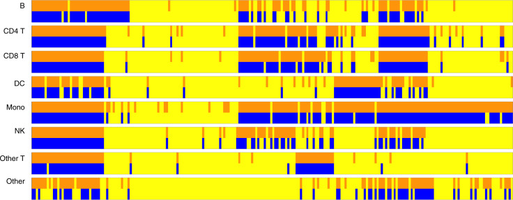
We first perform the hypothesis testing [2] by treating the proteins as Y and the top 5,000 genes as X. We then replace the top 5,000 genes by the marker genes and perform the same testing procedure. It turns out that the inference results are very similar. To better illustrate the similarity, we display the testing results row by row in Fig. 3: specifically, the odd rows represent the predictability using the top 5,000 genes, and the even rows represent the predictability using the marker genes. The columns represent the 226 proteins. Blue and orange bars highlight the protein/cell type combinations for which we reject H₀. The yellow bars indicate combinations for which H₀ is not rejected. Notably, the testing results for the two batches of genes are quite similar to each other: more than 93% of the tests reach the same conclusion. For the tests that disagree, 6.19% of the tests are the cases where the top 5,000 genes reject H₀ but the marker genes fail to reject. Those cases cover 10 proteins with their cell type given in SI Appendix, Table S1. For those cases, the interaction effects between the marker genes and other genes might provide additional prediction power. Besides, 0.22% of the tests are the cases where the marker genes reject H₀ but the top 5,000 genes fail to reject. We believe this is because increased noise in the data leads to inferior performance of the regression algorithm. It is also interesting to observe that among the 226 proteins, 22 proteins can be predicted in all cell types, and 31 proteins fail to be predicted in all cell types, based on the inference results using the top 5,000 genes. As for the marker genes, 13 proteins can be predicted in all cell types, and 42 proteins fail to be predicted in all cell types. In general, proteins with rich measurements can be predicted well.

Fig. 3.

The predictability test of every protein across all cell types. The columns represent the 226 proteins, and the row blocks represent the eight different cell types. In each cell type, the first row represents X being all 5,000 genes, and the second row represents X being the marker genes under the testing problem [2]. The orange bars and blue bars represent the tests rejecting H₀, and the yellow bars represent the tests failing to reject H₀.

To answer the second question, we let ${\mathcal{G}}_1$ represent the marker genes for each cell type. Then we remove the 1,692 marker genes from the set of top 5,000 genes and perform clustering analysis (21) for the remaining genes. We obtain 13 clusters, ${\mathcal{G}}_2,\hspace{0.17em}\dots ,\hspace{0.17em}{\mathcal{G}}_{14}$, the size of which decrease from hundreds to dozens. The goal is to test the prediction power of ${\mathcal{G}}_1,\hspace{0.17em}\dots ,\hspace{0.17em}{\mathcal{G}}_{14}$ on the proteins in each cell type.

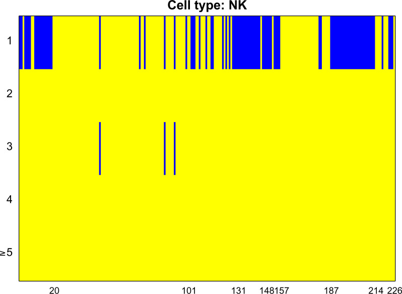
We begin by testing the prediction power of the marker genes (${\mathcal{G}}_1$) in each cell type. Specifically, each protein is treated as Y, and ${\mathcal{G}}_1$ is treated as Z in the testing problem [1]. Then, we test whether adding ${\mathcal{G}}_2,\hspace{0.17em}\dots$, or ${\mathcal{G}}_{14}$ to ${\mathcal{G}}_1$ improves the predictability of each protein. This is achieved by treating each of ${\mathcal{G}}_2,\hspace{0.17em}\dots$, or ${\mathcal{G}}_{14}$ as X in the testing problem [1]. We present the inference results for NK cells in Fig. 4 and relegate the other cell types to SI Appendix, Figs. S24–S30, where the P values are also adjusted by the Benjamini–Yekutieli method (20). Similarly, the blue bars represent the rejection of H₀, while the yellow bars represent the failure of rejection. The rows correspond to ${\mathcal{G}}_1,\hspace{0.17em}{\mathcal{G}}_2,\hspace{0.17em}\dots$, and the columns represent the proteins. As we expect, the marker genes are extremely useful in predicting the proteins. Adding extra gene clusters occasionally provides extra prediction power, and one protein (CD177) that is not predictable by marker genes is predictable with another gene cluster.

Fig. 4.

The predictability test of every proteins for NK cells. The first row represents the group marker genes ${\mathcal{G}}_1$, and the second to fifth rows represent the other clusters of genes ${\mathcal{G}}_2,\hspace{0.17em}{\mathcal{G}}_3,\hspace{0.17em}\dots$. We combine several clusters in the fifth row since the rejection of H₀ becomes rare.

SVG Detection

Background.

Recent technological advances in spatially resolved transcriptomics have enabled gene expression profiling with spatial information on tissues. The spatial transcriptomics sequencing technique measures the expression level for thousands of genes in different spots, which may contain multiple cells. The single molecule fluorescence in situ hybridization technique detects several messenger RNA (mRNA) transcripts simultaneously at the subcellular resolution but usually has relatively low expression levels compared to spatial transcriptomics. More recent technologies such as multiplexed error-robust FISH (MERFISH) (22) and sequential fluorescence in situ hybridization (23) can substantially increase the number of detectable mRNAs from hundreds to thousands.

The gene expression data are represented in an $n\times p$ matrix, where each column denotes a specific gene, and each row denotes an observed sample spot in the tissue. Each spot may contain one or multiple cells depending on the experimental method. The spot is also associated with a two-dimensional spatial location in the sample. It is of interest to identify the genes that display spatially distinct expression patterns. Similar to existing approaches (8, 10), we first test each gene separately, then control the false discovery rate based on the P values for all genes. For each gene, we denote its expression level as $Y=(Y_1,\dots ,Y_n)$ and the corresponding spatial location at the n spots as $X=(X_1,\dots ,X_n)$. In our numerical analysis, we let X_i be a four-dimensional covariate: intercept, horizontal coordinate, vertical coordinate, and the interaction effect of horizontal and vertical coordinate. Under the testing framework [2], we are interested in finding the genes that satisfy $\mathbb{E}(Y)\ne \mathbb{E}(Y|X)$.

Simulations.

We aim to determine via simulations if two versions of the proposed method (TT-S and TT-M) work well when compared with popular SVG methods, spatial pattern recognition via kernels (SPARK) (10) and SpaDE (8). Both methods are parametric models: SPARK assumes the gene expression follows Poisson distribution, and spatial gene expression patterns by deep learning of tissue images (SpaDE) assumes the data follow Gaussian distribution.

To generate synthetic data, we use the spatial location of the upcoming mouse olfactory bulb data and generate our spatial signals. Following ref. 10, we consider three spatial patterns: hot spot, gradient, and streak. A generic picture of all the three simulated models is illustrated in Fig. 5. The random forest algorithm is implemented in the regression step. We generate the signals according to the three patterns and add a random noise that follows the uniform distribution on $[0,1]$ to each spot. Specifically, denote the signal as $f(X_i)$, where X_i is the spatial information at location i. The gene expression at location i is generated by

$$Y_i=a\times f(X_i)+U_i,\hspace{1em}{U}_i\sim U(0,1).$$ [5]

Fig. 5.

The three spatial patterns for the gene expression in the simulation settings.

The details of $f(·)$ for each spatial pattern are given in SI Appendix. The signal level is controlled by the constant $a\in [0,1]$ in Eq. 5, where a = 0 implies the H₀ is true and a > 0 indicates that H₁ holds. Because the real data are sparse, we also consider the settings where we set Y _i = 0 if $Y_i<\text{median}(Y)$. Thus, 50% of all the locations are set to zero.

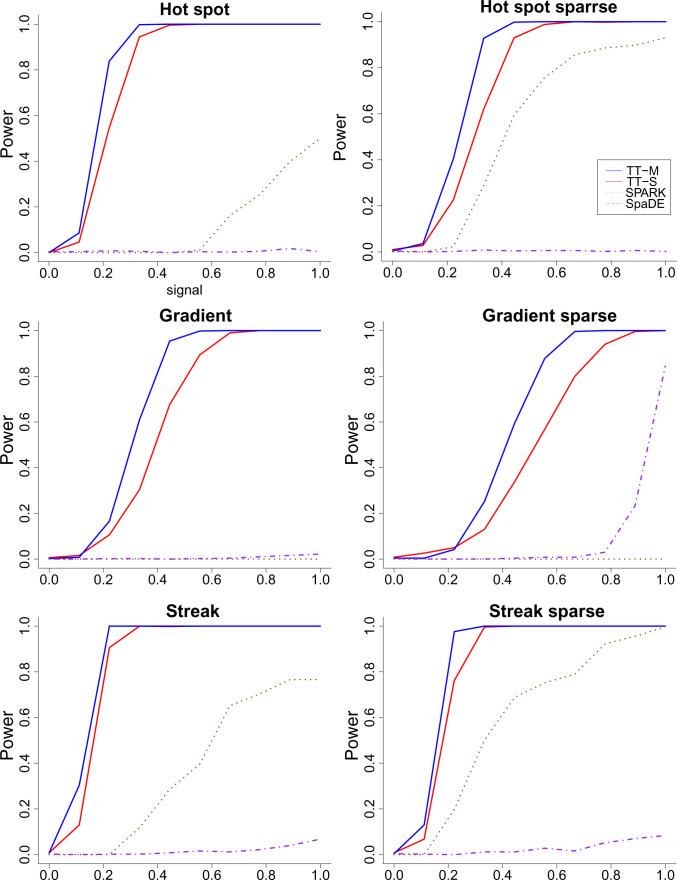
The simulation is repeated 1,000 times, and we report the average power for all the methods. The random forest algorithm is implemented as the regression tool, and we set the number of multiple splits to be 15. The power curves are illustrated in Fig. 6 where the type I error is set at 0.05. Additional simulation results are reported in SI Appendix. The y axis is the power, and the x axis is the signal level a. When a = 0, the null condition holds, and all methods can control the type I error very well. As a increases, the power also increases as expected. The proposed method shows superior performance across all settings: hot spot, gradient, and streak. The power curves also show that multiple splits are indeed more powerful compared to a single split under the alternative hypothesis. As the comparison between the two rows, we also find that all methods tend to perform better when the data are sparse, where half of the low expression levels are set to 0. This might be due to the low noise level under the sparse setting. SPARK tends to perform better than SpaDE under the hot spot and streak settings, and SpaDE outperforms SPARK when the signal is gradient. This finding also echos the simulation results in ref. 10 where SPARK and SpaDE have similar power only when the signal is gradient.

Fig. 6.

The power (vertical) versus signal (horizontal) for the regression-based two-sample t test, SPARK, and SpaDE when $\alpha =0.05$. (Top) Hot spot, (Middle) gradient, and (Bottom) streak patterns. (Left) Nonsparse and (Right) sparse settings. Across the 6 panels, the spatial patterns are as indicated in the main heading. Details provided in SI Appendix.

Next, we apply the proposed test to real datasets. The analyses illustrate that our proposed method produces calibrated P values under the null condition in the randomly permuted data and shows impressive power compared with existing approaches. We advocate the validity of our results since they do not require any distributional assumptions on the gene expression data and have less constraint when applied to real data. Because the real data analysis involves multiple testing, we adjust all the P values by applying the Benjamini–Yekutieli method (20) to control the false discovery rate at 5%. The choice of regression algorithm and the number of multiple splits are set to be the same as in the simulation.

Mouse Olfactory Bulb Data.

Spatial transcriptomics sequencing was used to produce the mouse olfactory bulb data (24). Following previous analyses using SpaDE (8) and SPARK (10), we used the MOB Replicate 11 file, which contains 16,218 genes measured on 262 spots. Similar to ref. 10, we filter out genes that are expressed in less than 10% of the array spots and select spots with at least 10 total read counts. After the filtering, we obtain 11,274 genes on 260 spots.

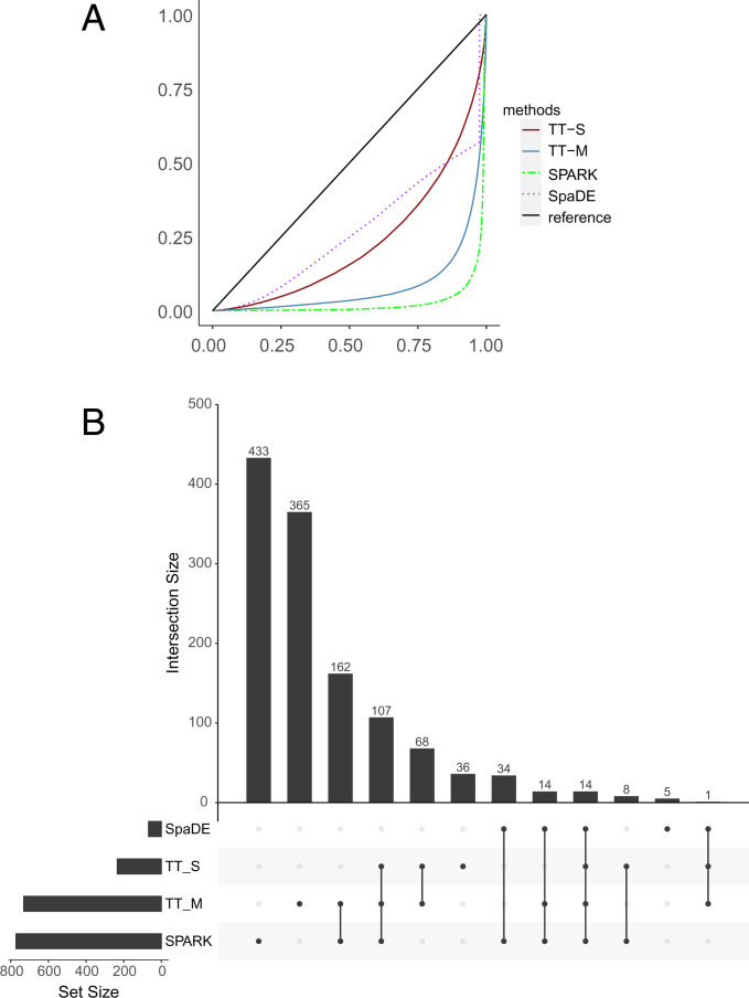
All methods produce valid P values under the null condition where the response is randomly permuted (Fig. 7A). With the original data, SPARK, SpaDE, TT-S, and TT-M identified 772, 68, 234, and 731 SVGs, respectively. More than 40% of the genes identified by TT-M overlap with SPARK (Fig. 7B). For the upset plot, the left bar plot represents the total size of each set, and the top bar plot represents the intersection of each method. Every possible intersection is shown by the bottom plot.

Fig. 7.

Analysis for the mouse olfactory bulb dataset. (A) The empirical distribution of the P values under the null condition in the permuted data. The solid blue line and solid red line denote the multiple splits (TT-M) and single splits (TT-S). The green dashed line denotes SPARK, and the purple dotted line denotes SpaDE. (B) The upset plot shows the overlap of genes for all the four methods. (Left) The total size of each set and (Top) the intersection of each method. (Bottom) Every possible intersection.

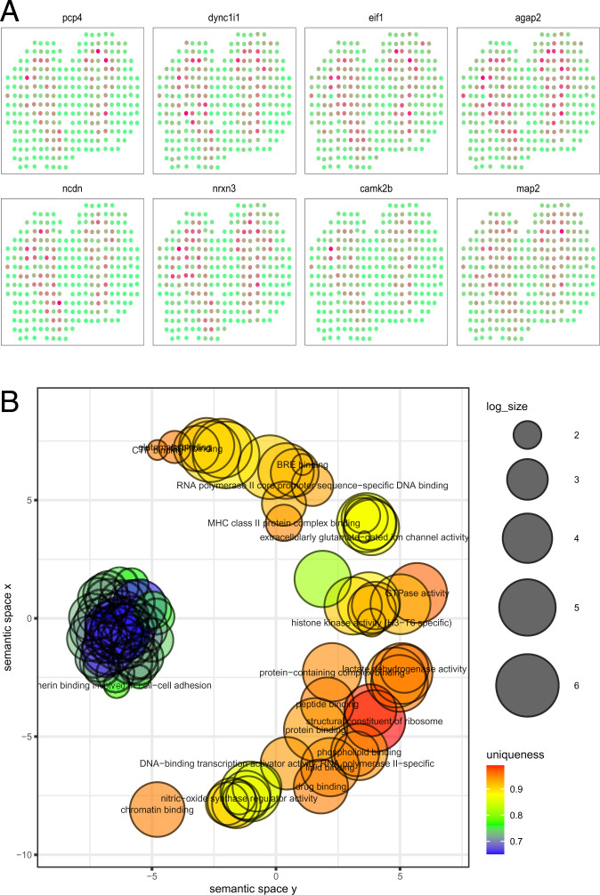
As an advantage of our method, we can check the variable importance of each feature as part of the random forest algorithm. Specifically, %IncMSE gives the increase in mean square prediction error as a result of the target variable being randomly permuted, and a larger value indicates relatively higher importance. In our data analysis, the average %IncMSE is 0.072 for the horizontal axis, 0.044 for the vertical axis, and 0.056 for the interaction effect of the horizontal and vertical axis. This indicates that most spatial variability in expression occurs across the horizontal axis as depicted by the most significant eight genes (Fig. 8A). The variation in expression is notable and approximately symmetric in the horizontal axis, indicating that the proposed method captures the variability in the spatial distribution accurately.

Fig. 8.

Analysis for the mouse olfactory bulb dataset. (A) The eight genes that have the smallest P values detected by TT-M. (B) The clustering of GO annotations for the genes detected by TT-M.

Last, we perform gene ontology (GO) enrichment analysis for molecular function and display the clustered GO annotations by implementing Revigo (25). The enrichment results offer an understanding of the SVGs detected by our method (Fig. 8B and SI Appendix, Figs. S12 and S13). Most of the detected genes are related to the binding of certain proteins or DNA. For example, the cluster on the left colored in blue and green represent the genes that are essential to cadherin binding in cell–cell adhesion. Our results complement the GO terms identified by SPARK, which are related to synaptic organization and olfactory bulb development.

Human Breast Cancer Data.

The human breast cancer data are also obtained by spatial transcriptomics sequencing (24). Following previous analyses using SpaDE (8) and SPARK (10), we use the Breast Cancer Layer 2 file, which contains 14,789 genes measured on 251 spots. We filter out the genes that are expressed in less than 10% of the array spots and selected spots with at least 10 total read counts. After filtering, we obtained 5,262 genes measured on 250 spots.

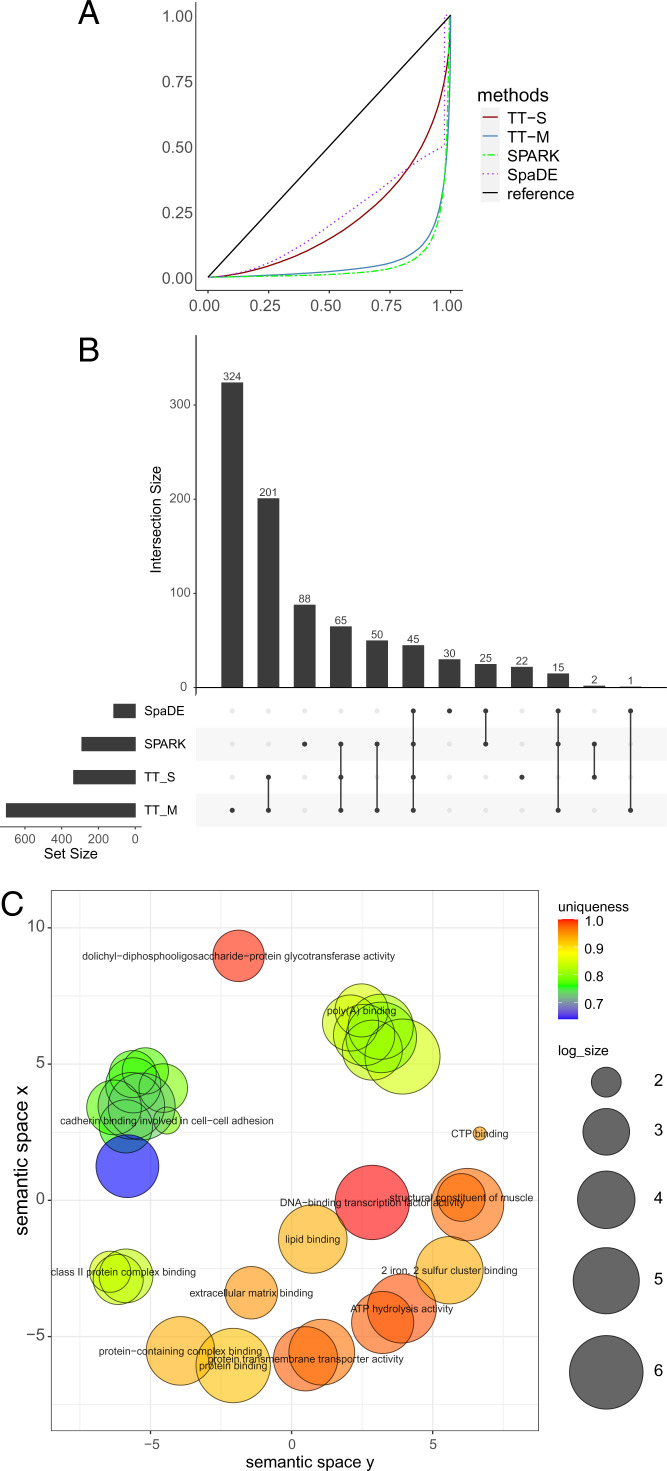
The results are summarized in Fig. 9. As expected, all methods produce valid P values under the null condition. SPARK identified 290 and SpaDE identified 115 SVGs. By comparison, TT-S identified 335 genes with more than 1/3 overlapping with SPARK, and TT-M identified 701 genes with around 1/4 overlapping with SPARK. Our proposed methods found considerably more genes compared to existing methods. We found that the breast cancer data have 23% of nonzero elements in the gene expression matrix, while the mouse olfactory bulb data have 56% of nonzero values. One possible explanation is that our methods are more powerful in picking up weak signals in sparse gene expression data.

Fig. 9.

Analysis for the human breast cancer data. (A) The empirical distribution of the P values under the null condition in the permuted data. The blue solid line and red solid line denote the multiple splits (TT-M) and single splits (TT-S). The green dashed line denote SPARK, and the purple dotted line denotes SpaDE. (B) The upset plot shows the overlap of genes for all the four methods. (C) The clustering of GO annotations for the genes detected by TT-M.

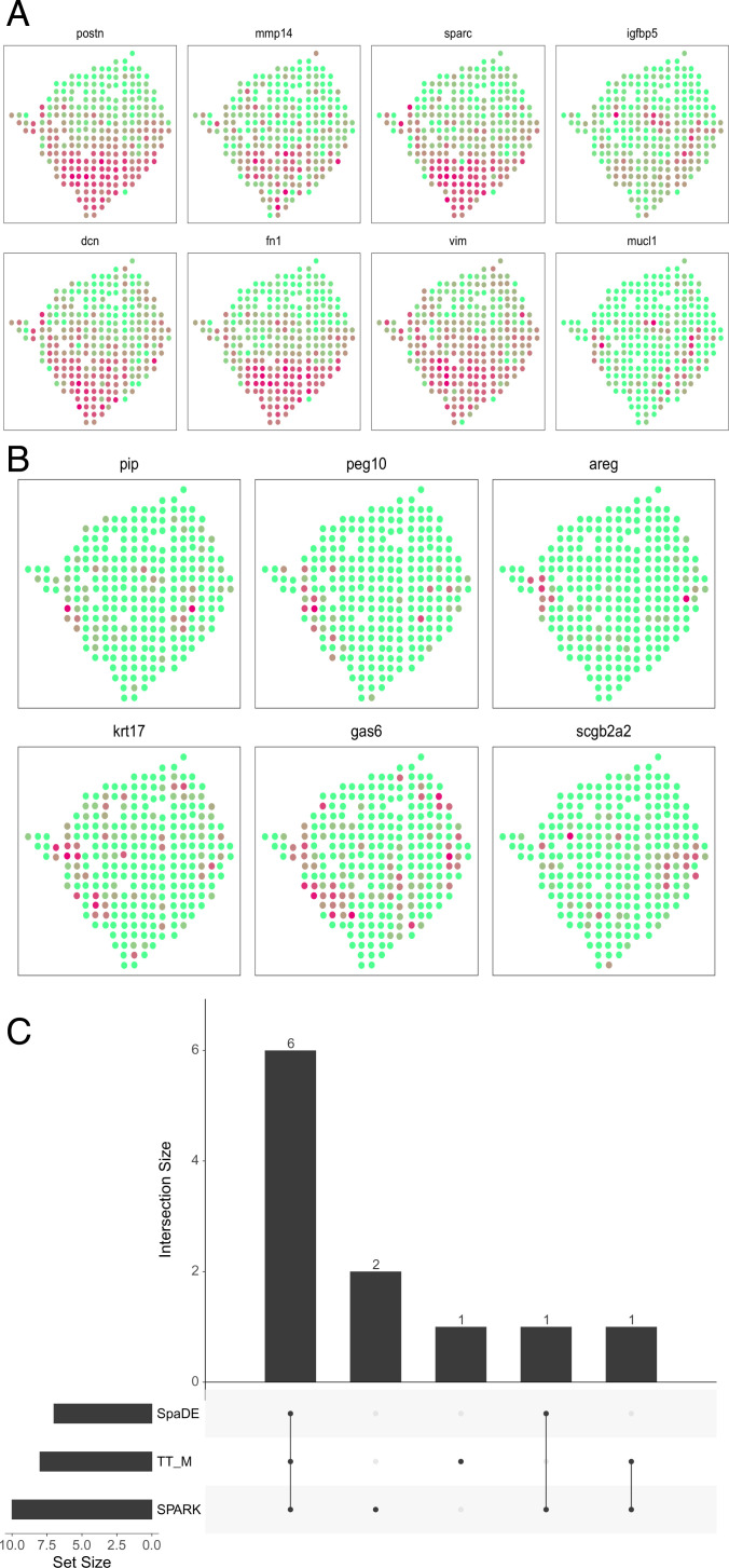
To provide additional evidence of the findings, we look into the overlaps of the detected genes with background information. We found 8 among the 14 cancer-related genes that are highlighted in the original study (24). SpaDE detected 7, and SPARK detected 9; see Fig. 10C for the overlaps of those genes. The gene expressions of the eight detected genes are illustrated in Fig. 10A, and the six missed genes are plotted in Fig. 10B. Clearly, the detected genes show strong spatial patterns. We also found 79 genes that are previously known to be related to cancer according to the CancerMine database (26). On the other hand, SpaDE detected 11, and SPARK detected 40.

Fig. 10.

Analysis of the cancer genes. (A) The 8 cancer genes that are detected by the proposed method as the SVGs among the 14 cancer genes highlighted in ref. 24. (B) The other six cancer genes that are missed by the proposed method. (C) The upset plot shows the overlap of the cancer genes for all three methods.

In terms of variable importance, the average %IncMSE equals 0.036 for the horizontal axis, 0.120 for the vertical axis, and 0.070 for the interaction effect of the horizontal and vertical axis. In contrast to the analysis of the mouse olfactory bulb data (Fig. 8A), the vertical axis plays a more important role in the spatial patterns. This phenomenon can be observed in the detected cancer genes shown in Fig. 10A. The enrichment results provide deep understanding of the detected SVGs (Fig. 9C and SI Appendix, Figs. S14 and S15). Most of the detected genes are also related to bindings of important cell functions and proteins.

Discussion

In this paper, we proposed an approach for the test of covariates and applied the method to test both prediction power in CITE-seq data and the identification of SVGs. Distinguished from previous methods, the proposed method does not assume any parametric distributions on the gene expression data, which provides great flexibility for real data analysis. We are also able to implement a large class of machine learning regression algorithms in the test, such as neural networks, random forest, SVM, etc.

Due to the sample splitting and machine learning algorithms, our test may not perform well when the sample size is too small. In the analysis of a small seqFISH data shown in SI Appendix, the proposed test found a relatively small number of SVGs. The sample size in these data is only 131. Thus, the effective sample size for training the random forest is only 65, which is not enough to obtain a properly trained algorithm.

The model-X knock-off (27) is a related model-free variable selection method. Our method differs from it in several important ways. First, the knock-off is used to evaluate the conditional dependence of each variable given all other covariates, while our method can be used to compare models of different nature. For example, our approach can easily compare linear regression and random forest to confirm that there is no uncaptured signal beyond linear relationships. Also, our method can be more suitable for a nested, sequential model exploration scenario. Second, the type I error control is different. While knock-off aims to control the false-positive rate in variable selection, our method provides family-wise error control by comparing each pair of candidate models. Third, our approach is more readily applicable to large-scale and complex data due to its simplicity. At the same time, knock-off requires the construction of exchangeable covariate pairs, which can be tricky if the covariate distribution is unknown.

There are several potential aspects of this work left for future research. For CITE-seq data, both the dimension and sample size are huge, and the design matrix is extremely sparse. This type of data presents unique challenges, and its analysis requires further development of theoretical and computational statistical tools. In spatial transcriptomic studies, the current literature on the test of SVGs is all based on single tests applied to each gene in the domain. The control of the false discovery rate is achieved by simply applying either qvalue (28) or the Benjamini–Yekutieli method (20). How to incorporate spatial information to achieve better false discovery control performance is a very promising future research topic. The idea proposed in this paper can also be applied to independence testing (16) or conditional independence testing (29) on multiomics data.

Data, Materials, and Software Availability

Previously published data were used for this work (4, 22–24). No new data were generated for this manuscript.

References

- 1.Fan J., Li R., Zhang C. H., Zou H., Statistical Foundations of Data Science (Chapman and Hall, 2020). [Google Scholar]
- 2.Zhou Z., Ye C., Wang J., Zhang N. R., Surface protein imputation from single cell transcriptomes by deep neural networks. Nat. Commun. 11, 651 (2020). [DOI] [PMC free article] [PubMed] [Google Scholar]
- 3.Davis D. M., Intercellular transfer of cell-surface proteins is common and can affect many stages of an immune response. Nat. Rev. Immunol. 7, 238–243 (2007). [DOI] [PubMed] [Google Scholar]
- 4.Hao Y., et al., Integrated analysis of multimodal single-cell data. Cell 184, 3573–3587.e29 (2021). [DOI] [PMC free article] [PubMed] [Google Scholar]
- 5.Gayoso A., et al., Joint probabilistic modeling of single-cell multi-omic data with totalVI. Nat. Methods 18, 272–282 (2021). [DOI] [PMC free article] [PubMed] [Google Scholar]
- 6.Stuart T., et al., Comprehensive integration of single-cell data. Cell 177, 1888–1902.e21 (2019). [DOI] [PMC free article] [PubMed] [Google Scholar]
- 7.Marx V., Method of the year: Spatially resolved transcriptomics. Nat. Methods 18, 9–14 (2021). [DOI] [PubMed] [Google Scholar]
- 8.Svensson V., Teichmann S. A., Stegle O., SpatialDE: Identification of spatially variable genes. Nat. Methods 15, 343–346 (2018). [DOI] [PMC free article] [PubMed] [Google Scholar]
- 9.Bernstein M. N., et al., Spatialcorr: Identifying gene sets with spatially varying correlation structure. bioRxiv [Preprint] (2022). https://www.biorxiv.org/content/10.1101/2022.02.04.479191v1 (Accessed 20 February 2022). [DOI] [PMC free article] [PubMed]
- 10.Sun S., Zhu J., Zhou X., Statistical analysis of spatial expression patterns for spatially resolved transcriptomic studies. Nat. Methods 17, 193–200 (2020). [DOI] [PMC free article] [PubMed] [Google Scholar]
- 11.Edsgärd D., Johnsson P., Sandberg R., Identification of spatial expression trends in single-cell gene expression data. Nat. Methods 15, 339–342 (2018). [DOI] [PMC free article] [PubMed] [Google Scholar]
- 12.Hu J., et al., SpaGCN: Integrating gene expression, spatial location and histology to identify spatial domains and spatially variable genes by graph convolutional network. Nat. Methods 18, 1342–1351 (2021). [DOI] [PubMed] [Google Scholar]
- 13.Zhu J., Sun S., Zhou X., SPARK-X: Non-parametric modeling enables scalable and robust detection of spatial expression patterns for large spatial transcriptomic studies. Genome Biol. 22, 184 (2021). [DOI] [PMC free article] [PubMed] [Google Scholar]
- 14.Li Q., Racine J. S., Nonparametric Econometrics: Theory and Practice (Princeton University Press, 2007). [Google Scholar]
- 15.Lei J., Cross-validation with confidence. J. Am. Stat. Assoc. 115, 1978–1997 (2020). [Google Scholar]
- 16.Cai Z., Lei J., Roeder K., A distribution-free independence test for high dimension data. arXiv [Preprint] (2021). https://arxiv.org/abs/2110.07652 (Accessed 20 December 2022).
- 17.Liu Y., Xie J., Cauchy combination test: A powerful test with analytic p-value calculation under arbitrary dependency structures. J. Am. Stat. Assoc. 115, 393–402 (2020). [DOI] [PMC free article] [PubMed] [Google Scholar]
- 18.Chen T., Guestrin C., “Xgboost: A scalable tree boosting system” in Proceedings of the 22nd ACM SIGKDD International Conference on Knowledge Discovery and Data Mining (Association for Computing Machinery, 2016), pp. 785–794.
- 19.Shao X., Zhang J., Martingale difference correlation and its use in high-dimensional variable screening. J. Am. Stat. Assoc. 109, 1302–1318 (2014). [Google Scholar]
- 20.Benjamini Y., Yekutieli D., The control of the false discovery rate in multiple testing under dependency. Ann. Stat. 29, 1165–1188 (2001). [Google Scholar]
- 21.Morabito S., et al., Single-nucleus chromatin accessibility and transcriptomic characterization of Alzheimer’s disease. Nat. Genet. 53, 1143–1155 (2021). [DOI] [PMC free article] [PubMed] [Google Scholar]
- 22.Moffitt J. R., et al., Molecular, spatial, and functional single-cell profiling of the hypothalamic preoptic region. Science 362, eaau5324 (2018). [DOI] [PMC free article] [PubMed] [Google Scholar]
- 23.Shah S., Lubeck E., Zhou W., Cai L., In situ transcription profiling of single cells reveals spatial organization of cells in the mouse hippocampus. Neuron 92, 342–357 (2016). [DOI] [PMC free article] [PubMed] [Google Scholar]
- 24.Ståhl P. L., et al., Visualization and analysis of gene expression in tissue sections by spatial transcriptomics. Science 353, 78–82 (2016). [DOI] [PubMed] [Google Scholar]
- 25.Supek F., Bošnjak M., Škunca N., Šmuc T., REVIGO summarizes and visualizes long lists of gene ontology terms. PLoS One 6, e21800 (2011). [DOI] [PMC free article] [PubMed] [Google Scholar]
- 26.Lever J., Zhao E. Y., Grewal J., Jones M. R., Jones S. J. M., CancerMine: A literature-mined resource for drivers, oncogenes and tumor suppressors in cancer. Nat. Methods 16, 505–507 (2019). [DOI] [PubMed] [Google Scholar]
- 27.Candes E., Fan Y., Janson L., Lv J., Panning for gold: ‘Model-x’ knockoffs for high dimensional controlled variable selection. J. R. Stat. Soc. Ser. B Stat. Methodol. 80, 551–577 (2018). [Google Scholar]
- 28.Storey J. D., The positive false discovery rate: A Bayesian interpretation and the q-value. Ann. Stat. 31, 2013–2035 (2003). [Google Scholar]
- 29.Cai Z., Li R., Zhang Y., A distribution free conditional independence test with applications to causal discovery. J. Mach. Learn. Res. 23, 1–41 (2022). [Google Scholar]
Associated Data
This section collects any data citations, data availability statements, or supplementary materials included in this article.
Supplementary Materials
Data Availability Statement