

Abstract
Background:
This paper represents, to our knowledge, the first national-level (United States) estimate of the economic impacts of vibriosis cases as exacerbated by climate change. Vibriosis is an illness contracted through food- and waterborne exposures to various Vibrio species (e.g., nonV. cholerae O1 and O139 serotypes) found in estuarine and marine environments, including within aquatic life, such as shellfish and finfish.
Objectives:
The objective of this study was to project climate-induced changes in vibriosis and associated economic impacts in the United States related to changes in sea surface temperatures (SSTs).
Methods:
For our analysis to identify climate links to vibriosis incidence, we constructed three logistic regression models by Vibrio species, using vibriosis data sourced from the Cholera and Other Vibrio Illness Surveillance system and historical SSTs. We relied on previous estimates of the cost-per-case of vibriosis to estimate future total annual medical costs, lost income from productivity loss, and mortality-related indirect costs throughout the United States. We separately reported results for V. parahaemolyticus, V. vulnificus, V. alginolyticus, and “V. spp.,” given the different associated health burden of each.
Results:
By 2090, increases in SST are estimated to result in a 51% increase in cases annually relative to the baseline era (centered on 1995) under Representative Concentration Pathway (RCP) 4.5, and a 108% increase under RCP8.5. The cost of these illnesses is projected to reach annually under RCP4.5, and annually under RCP8.5, relative to in the baseline (2018 U.S. dollars), equivalent to 140% and 234% increases respectively.
Discussion:
Vibriosis incidence is likely to increase in the United States under moderate and unmitigated climate change scenarios through increases in SST, resulting in a substantial burden of morbidity and mortality, and costing billions of dollars. These costs are mostly attributable to deaths, primarily from exposure to V. vulnificus. Evidence suggests that other factors, including sea surface salinity, may contribute to further increases in vibriosis cases in some regions of the United States and should also be investigated. https://doi.org/10.1289/EHP9999a
Introduction
Scientific evidence demonstrates that human-influenced climate change is occurring and is taking its toll on environmental and public health in numerous ways. Globally, air and ocean temperatures are increasing, mean sea level is rising, and extreme weather events are becoming more common and more severe.1,2 The human health outcomes related to these changes are costly. For instance, Limaye et al. documented that 10 climate-sensitive events that occurred in the United States in 2012 resulted in direct and indirect health-related costs of (2018 U.S. dollars).3 Beyond distinct events, climate change is impacting the prevalence, ranges, and concentrations of food- and waterborne pathogens, such as those in the genus Vibrio.4–6 Accurate projections of vibriosis incidence and the future costs of associated health outcomes are important for informing policies designed to prevent or mitigate the impacts of climate change.3
Although cholera (infection from V. cholerae) is the most well-known type of illness resulting from exposure to any type of Vibrio bacteria, it is relatively uncommon in the United States and generally is linked to international travel.7,8 Other nonV. cholerae Vibrio species are more common causes of health impacts in the United States.5,9,10 V. parahaemolyticus, V. alginolyticus, and V. vulnificus are generally among the most prevalent species of Vibrio in the United States and are the primary sources of noncholera vibriosis, the illness resulting from exposure to noncholera-causing Vibrio species.7 Moreover, V. parahaemolyticus and V. vulnificus are among the most common sources of domestic seafood-related food poisoning cases in the United States. V. parahaemolyticus is responsible for the greatest number of domestic Vibrio-related cases per year.9,10 V. vulnificus has the highest mortality rate of all seafood-borne pathogens in the United States.11,12 Health outcomes from exposure to Vibrio species range from mild gastroenteritis and “swimmer’s ear,”13 to more severe outcomes, such as necrotizing fasciitis, amputation, septicemia, and death.8 Many of the worst outcomes occur in men of age with preexisting hepatic or renal disease, including cirrhosis, diabetes mellitus, hepatitis, or cancer.12,14 Exposures to Vibrio species typically occur through oral or dermal routes, most commonly through consumption of raw or undercooked seafood (typically, raw oysters), ingestion of contaminated water, or via dermal exposures when the bacteria enter the body through cuts in the skin.15
Understanding the biological effects of climate change on different Vibrio species (Vibrio spp.) is critical to protecting public health in the United States and globally, as is the ability to project related impacts on infection incidence rates.16–18 The life cycles of Vibrio spp., as well as their range and geographic prevalence, are tied to climate conditions, including sea surface temperature (SST), which will likely rise with climate change.19 Data show an increase in the incidence of vibriosis occurring from exposures to V. parahaemolyticus and V. vulnificus since the 1970s9,20; additionally, infections from other Vibrio species, including V. alginolyticus, are rising in the United States,21 with further increases expected in the future from warming coastal waters.22 Internationally, heat waves and severe weather have been linked to increases in vibriosis infection rates.23,24 In the United States, Logar-Henderson et al.25 showed an increased risk of vibriosis in the 12-month period during and following an El Niño, when ocean temperatures rise. Davis et al.26 demonstrated that shallower intertidal areas of the Puget Sound with warmer air temperatures and SST have greater concentrations and growth rates of pathogenic strains of V. parahaemolyticus, thus leading to greater vibriosis risk. Because climate change is expected to continue increasing SST in coastal areas of the United States, there is concern that this also may affect vibriosis rates.19
This paper examines the implications of these changes by presenting a novel analysis of the climate-induced impacts on vibriosis cases caused by all nonV. cholerae species in the United States. It looks at the direct link between domestic disease incidence and SST. To perform this analysis, we statistically modeled the relationship between historical SSTs and reported vibriosis cases after linking incidents of illness with coastal exposure locations. Using the model estimates and predicted SSTs throughout the 21st century under various climate scenarios, we then estimated the number of future vibriosis cases. Finally, we valued the direct and indirect health-related costs of those cases, separately by Vibrio species. Our climate and socioeconomic scenarios were consistent with those adopted for the U.S. Environmental Protection Agency’s (EPA) Climate Change Impacts and Risk Analysis (CIRA) framework,27,28 designed to enable systematic quantification and valuation of climate change–attributable damages across multiple U.S. sectors (e.g., human health, infrastructure, water resources) and to facilitate the comparison and aggregation of results across affected sectors.
Methods
Our analysis quantified and valued changes in vibriosis resulting from rising SSTs throughout the 21st century. Each of the following steps of our analysis are described in the following sections:
Associated vibriosis cases with the coastal counties where the exposure occurred between 2007 and 2018 (section “Historical Vibriosis Case Data and Exposure Counties”)
Processed SST to identify historical monthly average values in coastal counties (section “Historical SST and Other Climate Data”)
Estimated a health impact function to model the historical relationship between SST and vibriosis (section “Model Historical Relationship between SST and Vibriosis”)
Estimated future SST using projected future increases in air temperatures in coastal counties (section “SST Projections”)
Predicted future probability of vibriosis infections throughout the 21st century using the health impact function (step 3) and future projections of SST (step 4), which were then scaled to the number of cases using multipliers derived from historical case data (section “Project Future Vibriosis Illness from Future Climate”)
Valued the direct and indirect costs of future vibriosis illnesses from the available literature (section “Estimate Economic Impact of Future Vibriosis”).
Institutional review board and ethics approval was not required. This study used publicly available data and did not meet the criteria for human subjects research.
Historical Vibriosis Case Data and Exposure Counties
This analysis relied on reported vibriosis data from the Centers for Disease Control and Prevention’s (CDC) Cholera and Other Vibrio Illness Surveillance (COVIS) system,29 the output of a national-level surveillance system for vibriosis and cholera. Between 1997 and 2006 only cholera was nationally notifiable, which is when most states began reporting cases. Starting in 2007, vibriosis became nationally notifiable as well, meaning the data contain all diagnosed cases of vibriosis.
Through the standardized COVIS reporting form, participating health agencies provided information about the patient’s history of seafood consumption and exposure to water bodies, as well as traceback information on implicated seafood. Importantly, some of this information provided data that could be linked with the geographic exposure location (i.e., the location of the Vibrio species that ultimately caused a human infection), as opposed to the location of the reporting health department. We assigned each case to an exposure county by undertaking a rigorous and systematic data screening effort. For confirmed and probable foodborne cases, we relied on harvest site information recorded as part of supplemental seafood investigation efforts. In some cases, these sites were coded as shellfish management areas, with observable boundaries easily matched with coastal counties. In other cases, other geographic information (e.g., names of water bodies) were provided, which required manually matching with coastal counties. We also explored, but ultimately did not use, shippers’ locations when the location of the harvest site was missing. In cases where both shipper’s location and harvest site location were given, we found a low level of correlation (i.e., 44% of cases where the harvester and shipper were in the same county), meaning shipping location would not serve as a suitable proxy for exposure location. For confirmed and probable nonfoodborne cases, we used any available information on out-of-state travel destinations, any interactions with water bodies, and the identified location of waterborne exposure to assign exposure location. These geographic identifiers were matched with county names by referencing maps. Given the inconsistency with which geographic information was recorded and the variation in level of detail provided in COVIS, we were able to identify exposure locations for only 4,023 of 14,017 recorded vibriosis infections matched with the 323 coastal counties (29%). Although it is possible that the absence of exposure location information in COVIS is nonrandom, we did not expect the relationship was correlated with SST or any other environmental factors that would influence our analysis.
Historical SST and Other Climate Data
The National Oceanic and Atmospheric Administration’s (NOAA) National Oceanic Optimum Interpolation Sea Surface Temperature Version 2 (OISSTV2) data set provides satellite and model-interpolated analysis of SST using a consistent methodology back to September 1981 and is publicly available.30 These data have been used in other Vibrio work, such as Semenza et al.,31 and provide global daily values of SST at a 1/4-degree spatial resolution. Sea surface salinity (SSS) data, writ large or in sufficiently complete formats, are not as widely available as SST data, as discussed in the section “Model Historical Relationship between SST and Vibriosis.” To develop the data set used in this study, we compiled two sources covering different time periods, depending on availability. The first source was derived from the Aquarius SSS optimal interpolation analysis, L2 (version 5.0) developed at the International Pacific Research Center of the University of Hawaii.32 This data set is provided weekly at a 1/2-degree resolution, and we used it for the period from April 2011 to April 2015. For the period from May 2015 to June 2019, we used the Soil Moisture Active Passive platform, SSS L3 (version 4.0), developed by both National Aeronautics and Space Administration and Remote Sensing Systems.33,34 These gridded data sets were spatially aggregated to counties using nearshore areas of each coastal county and aggregated to a monthly time step if monthly averages were not provided by the source. Nearshore air temperature data were also processed for all coastal counties but were too highly correlated with SST to include as a separate covariate in the model described in the next section [correlation for the contiguous United States (CONUS) specifically].
Model Historical Relationship between SST and Vibriosis
To estimate the relationship between SST and vibriosis incidence, this analysis constructed separate statistical models by Vibrio species group (par, vul, alg, and other), where each observation represented vibriosis incidence in exposure county c in coastal state s in month m during year y. In our data, we found very little variation in the number of cases linked to each exposure location by month; therefore, we converted the total number of cases to a binary outcome variable identifying instances where any vibriosis case was recorded. To estimate the models, we used logistic regression, which often is employed in health impact function modeling where the outcome variable is dichotomous and is observed with limited frequency.35 These models take the following forms:
| (1) |
| (2) |
| (3) |
| (4) |
The main explanatory variable of interest was SST. Because different Vibrio species have unique temperature ranges in which they thrive, this analysis considered threshold levels identified in the literature and created separate functional forms for SST by species group. For instance, V. parahaemolyticus grow well in SSTs and up to .36 Thus, our treatment of SST in Equation 1 started at 8°C and included the full range of our data given that 45°C is beyond the maximum in our data set. For V. vulnificus, the literature establishes an optimal growth range of 13–20°C, although the species still may be present at higher temperatures.37 Therefore, in Equation 2, we separately considered the relationship over the 13–20°C and the ranges, using a linear spline with a knot at 20°C. For V. alginolyticus, growth ranges are similarly wide. Given evidence that growth can occur at temperatures of as low as 5°C,38 and that 22°C may also be an important threshold value,39,40 in Equation 3, we separately considered the relationship within the 5–22°C and the ranges, using a linear spline with a knot at 22°C. Finally, in Equation 4, we included the full range of SST without reference to optimal growth ranges given the heterogeneity in conditions across the many species included in this group. In addition to considering the aforementioned growth ranges from the literature, we also explored the nonparametric relationships between SST and vibriosis incidence using locally weighted robust scatterplot smoothing (LOWESS) functions.
The models also controlled for other geographic variation using state fixed effects and temporal variation using year fixed effects (where the base year is the most recent year, 2018). State fixed effects controlled for time-invariant environmental conditions, as well as institutional considerations, such as Vibrio control and management plans that may reduce exposure to the bacteria by imposing restrictions on the seafood industry or recreation. Year fixed effects controlled for any potential reporting bias in earlier years when awareness of vibriosis was more limited and misdiagnosis may have been more common or where changes in testing regimes over time may have led to increased diagnoses. To account for correlation across observations within a given coastal county, we clustered standard errors (SEs) at the county level (e.g., Eicker41; Huber42). Finally, represented the error term. We considered results to be statistically significant at -values of 0.100 or smaller. To empirically investigate the importance of SSS, we estimated an additional model that included a contemporaneous SSS measure for the subsample of time for which this information is available.
SST Projections
Projections of future SST followed the framework and data sets used in other U.S. EPA CIRA studies to maximize consistency for cross-comparison with other estimates. For all coastal counties, we used a straightforward bias correction technique commonly called the delta method, where modeled temperatures for the projection period are compared with historical modeled temperatures to develop a difference between the two periods, or delta. These differences in temperature were then added to the historical mean from the baseline period (1986–2005). Baseline SST—using NOAA’s OISSTV2—was combined with differences (or deltas) in temperature at the county scale in three regions: CONUS states, Alaska, and Hawaii.30 In all cases, we used both Representative Concentration Pathways (RCP) 4.5 and 8.5, which represent low and high greenhouse gas emissions scenarios, respectively.43 We applied different general circulation models (GCMs) for the CONUS states, Alaska, and Hawaii, based on models and data sets used in other U.S. EPA CIRA framework studies. The deltas were calculated using downscaled air temperatures44 for the CONUS states, downscaled air temperatures for Alaska,43 and raw GCM SST output (consistent with Lane et al.45) for Hawaii.
In particular, for the CONUS states, we used a subset of the GCMs generated for the Intergovernmental Panel on Climate Change’s Fifth Assessment Report (AR5): CanESM2, CCSM4, GISS-E2-R, HadGEM2-ES, MIROC5, and GFDL-CM3, chosen to represent a broad range of climate projections, as described by the U.S. EPA.28 These projections were downscaled using a statistically based process that employs a multiscale spatial matching scheme44 at a spatial resolution of 1/16 degree. From these, we used monthly air temperature changes from the baseline, spatially aggregated along the coastline of each coastal county to construct the differences in temperature that we applied to the historical SSTs. For Alaska, we used the same approach as for the CONUS states but using a different set of GCMs with a bias correction procedure developed by the Scenarios Network for Planning (SNAP), a part of the International Arctic Research Center at the University of Alaska Fairbanks.46 GCMs in SNAP included the CCSM4, GFDL-CM3, GISS-E2-R, IPSL-CM5A-LR, and MRI-CGCM3. Finally, for Hawaii, we calculated deltas from annual raw GCM SST output, using the model hindcast and projection period, consistent with Lane et al.45 The annual differences in near-coast SSTs were applied to the monthly mean SSTs such that the seasonality from the historical period remained constant but the annual mean shifted along with the annual deltas. The projections for Hawaii did not include any projected shifts in the seasonality, which were included for the other states. The set of GCMs used for Hawaii were CanESM2, CCSM4, GISS-E2-R, HadGEM2-ES, and MIROC5.
Project Future Vibriosis Illness from Future Climate
We employed the estimated coefficients from Equations 1–4 to project future vibriosis cases linked to climate change using the CIRA framework. Given the nonlinear forms of our models, the regression output was transformed to predict probabilities of vibriosis, where the probabilities ranged from 0 to 1. Because the predictions were related to future time periods, we included all estimated coefficients except the year fixed effects in our prediction functions (thereby assuming a base year of 2018, under the new reporting regime) as follows:
| (5) |
| (6) |
| (7) |
| (8) |
To estimate the number of cases from these probabilities, we made several corrections. First, we multiplied the estimated probabilities from Equations 5–8 by the relationship between the number of county and month combinations where Vibrio was identified as a cause of illness (i.e., values of 1 in our historical data set) and the total number of reported cases identified in COVIS between 2007 and 2018. For instance, there were 1,573 V. vulnificus cases identified in the full COVIS data set, which we linked to 593 exposure county and month combinations, resulting in a multiplier of 2.65. The multipliers were 4.99 for V. parahaemolyticus (5,519 total cases and 1,106 county and month combinations), 2.84 for V. alginolyticus (2,209 total cases and 777 county and month combinations), and 8.78 for V. spp. (4,716 total cases and 537 county and month combinations).
Then, we made several adjustments following the modeling by Scallan et al.6 This included accounting for underreporting by multiplying estimated reported cases by 1.1 across all species.6 Similarly, this included accounting for underdiagnosis with additional multipliers, including 142.4 for V. parahaemolyticus, 142.7 for V. alginolyticus and V. spp., and 1.7 for V. vulnificus.6 Finally, we removed cases likely linked with international travel, including 2% of all V. vulnificus cases, 10% of V. parahaemolyticus cases, and 11% of V. alginolyticus and V. spp. cases.6 For example, across all Scallan et al.6 correction factors, V. parahaemolyticus cases predicted by our model using COVIS data were multiplied by 1.1, 142.4, and 0.90, to arrive at a final estimate of total cases linked with domestic exposure.
Estimate Economic Impact of Future Vibriosis
We used the U.S. Department of Agriculture’s (USDA) Cost Estimates of Foodborne Illnesses data product,47 which is based on multiple sources of information and prior research documented by Hoffmann et al.48 and Batz et al.49 to estimate the expected health outcomes from each infection estimated in the section “Project Future Vibriosis Illness from Future Climate” by species. The USDA work estimated the per-case cost of illnesses diagnosed as having been caused by Vibrio vulnificus, V. parahaemolyticus, and V. spp. Its per-case costs estimates are not affected by route of exposure. Outcomes included a) cases that did not seek medical attention; b) cases that involved a visit with a physician and recovery; c) cases that resulted in hospitalization, distinguished between those involving sepsis and those that were not involving sepsis (not sepsis); d) posthospitalization recovery (sepsis and not); and e) premature death. Sepsis was broken out because hospitalizations involving sepsis are more severe, longer, and more expensive than those without sepsis. We assumed levels of medical treatment and recovery happen sequentially. For example, one person with an infection may recover without medical care. Another may start by seeking outpatient care that leads to hospitalization with sepsis, followed by a longer posthospitalization recovery period. The USDA estimates the proportion of total species cases that pass through each of these branches of species-specific disease outcomes trees.47 Three major types of costs were included: direct medical costs, indirect productivity losses (decrease in the value of time owing to illness), and the value of premature mortality. Because V. alginolyticus was not modeled as a separate species and was therefore included in the V. spp. model,47 we applied the V. spp. costs to V. alginolyticus cases as well.
Consistent with federal guidance,50 we did not project changes in real medical treatment costs over time. In the absence of willingness-to-pay estimates to avoid time-losses from vibriosis, we valued the opportunity cost of this time using the median daily wage rate in the U.S. EPA’s Environmental Benefits Mapping and Analysis Program (BenMAP, which obtained wage rates from the U.S. Census Bureau’s 2015 American Community Survey). This rate was converted to 2018 U.S. dollars using the Employment Cost Index compiled by the U.S. Bureau of Labor Statistics and adjusted for future years using a per capita gross domestic product (GDP) adjustment factor, resulting in the following daily wage values: in 2030, in 2050, in 2070, and in 2090 (in undiscounted 2018 U.S. dollars). This approach was consistent with economic analysis guidance and approaches employed by the U.S. EPA50–52 and the USDA.47 Finally, to value premature mortality for the portion of cases that result in death, we used the value of statistical life (VSL) from the U.S. EPA’s “Guidelines for Preparing Economic Analyses,” which recommends a value of (2008 U.S. dollars) based on 1990 incomes.50 We then adjusted for future inflation and income growth using a forecast of GDP from the Emissions Predictions and Policy Analysis model (version 6)53 and accounted for population projections from Integrated Climate and Land-Use Scenarios (ICLUS) project (version 2), a county-level population projection adopted for CIRA work.28 The approach we employed is consistent with other studies examining the health effects of climate change, including Achakulwisut et al.54 and Gorris et al.55 It yielded the following VSL values: in 2030, in 2050, in 2070, and in 2090 (in undiscounted 2018 U.S. dollars).
Results
This section describes the results of our treatment of the historical Vibrio case data (section “Historical Vibrio Case Data and Exposure Counties”), our regression model identifying the historical relationship between SST and vibriosis (section “Historical Relationship between SST and Vibriosis”), projected number of future vibriosis cases under future SST (section “Projected Vibriosis under Future Climate Conditions”), and the estimated economic impact of those future cases (section “Estimate Economic Impact of Future Vibriosis”) (see also below).
Historical Vibrio Case Data and Exposure Counties
Between 2007 and 2018, the COVIS data identified 14,225 Vibrio infections across the United States, 14,017 (99%) of which were from nonV. cholerae species, the focus of our analysis. Figure 1 describes the trends in reported vibriosis cases in the United States over this time frame, as well as the variation in reported cases by species. Since data first became nationally reportable in 2007, V. parahaemolyticus has been the most prevalent species, with totals equivalent to the aggregate across all other nonV. cholerae species. Reported cases of V. vulnificus hover between 100 and 200 per year, and cases of V. alginolyticus have reached nearly 300 confirmed cases annually in recent years. In 2017 and 2018, there were significant increases in reported cases that did not identify a species, which we included in the V. spp. category. The V. spp. group includes over 20 species other than V. cholerae, V. parahaemolyticus, V. vulnificus, and V. alginolyticus.
Figure 1.

Trends identified in vibriosis cases in the United States reported to COVIS (2007–2018) by species. This figure does not present the number of total cases, which would account for underreporting and misdiagnosis. See Table S14 for the corresponding values presented in this figure. Note: ALG, V. alginolyticus; COVIS, Cholera and Other Vibrio Illness Surveillance (system); OTHER, other non V. cholerae Vibrio species, including V. cholerae non-O1 and non-O139, V. cincinnatiensis, V. damsela, V. fluvialis, V. furnissii, V. hollisae, V. metschnikovii, V. mimicus, V. species not identified, multiple V. species, and other; PAR, V. parahaemolyticus; VUL, V. vulnificus.
Figure 2 provides the geographic distribution of cases by reporting county based on COVIS and the more focused distribution of exposure county locations of vibriosis cases identified through the screening process. It shows that considering only the reporting location linked to a case very likely misattributes the environmental conditions associated with the exposure pathway. Identifying cases to the county of exposure provides a more direct relationship to the county average SST.
Figure 2.
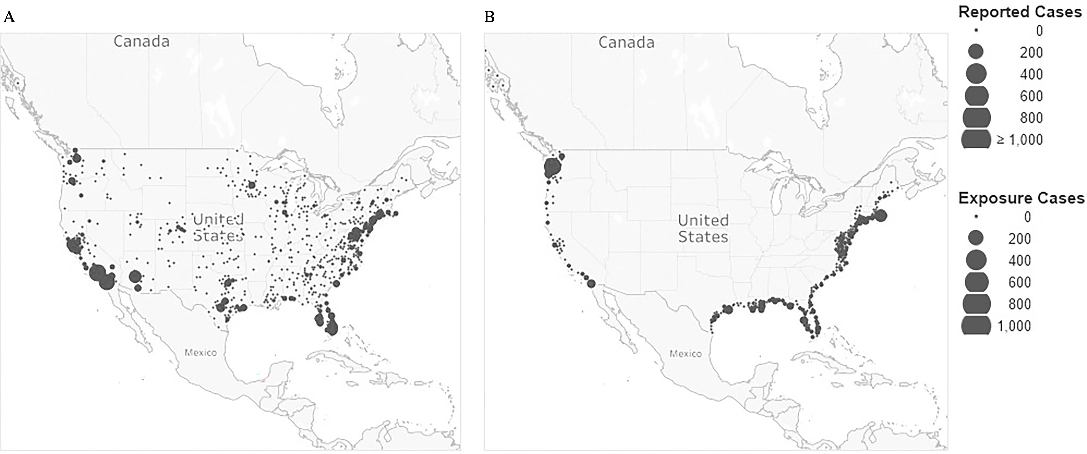
Geographic distribution of vibriosis cases in the United States reported to COVIS (2007–2018) by (A) reporting county and (B) county of exposure identified during the screening analysis. COVIS case data shown here include all nonV. cholerae Vibrio species. Individual county totals are symbolized at the county centroid. The data from COVIS include all confirmed, confirmed and probable, and probable cases recorded from the contiguous 48 states, Hawaii, and Alaska. Given the inconsistency with which geographic information is recorded and the variation in level of detail provided in COVIS, the number of identified exposure locations matched with the 323 coastal exposure counties (29%) was 4,023 of 14,017 total recorded vibriosis infections. Map created in Tableau Desktop, Professional Edition (2021.4.3). The base map is 2022 Mapbox; OpenStreetMap. Note: COVIS, Cholera and Other Vibrio Illness Surveillance (system).
Our investigation of the historical COVIS data also considered several other features of the data. For example, we found that most vibriosis infections occur in May through September (Figure S1). The data also revealed differences in food- and nonfoodborne transmission pathways by species (Table S1), as well as by county of exposure (Figure S2). For instance, the data showed that V. parahaemolyticus and V. spp. are more likely associated with foodborne transmission, whereas V. vulnificus and V. alginolyticus are more frequently linked with nonfoodborne exposure. Geographic differences by species and across regions also could be inferred across the exposure county locations (Figures S3 and S4).
Historical Relationship between SST and Vibriosis
Table 1 summarizes results specific to the SST variables for each of the three species models. For the V. parahaemolyticus model, we identified a statistically significant positive relationship between SST and the likelihood of vibriosis illness for the range (, , ). Likewise for V. vulnificus, we observed a statistically significant positive relationship for the 13–20°C range (, , ), and the range (, , ), where the coefficient on the former temperature range was more than twice as large as the latter. Similarly, the model for V. alginolyticus demonstrated a statistically significant positive relationship over the 5–22°C temperature range (, , ) and range (, , ), with a steeper slope among the lower range. For each of the V. parahaemolyticus, V. vulnificus, and V. alginolyticus models, we attempted separate specifications that also included variables for the excluded temperature range below the thresholds (e.g., for V. parahaemolyticus, for V. vulnificus, for V. alginolyticus) and found that none of these coefficients were statistically significant ( for V. parahaemolyticus, for V. vulnificus, and for V. alginolyticus), thus demonstrating that these Vibrio species indeed are unlikely to thrive below the thresholds identified in the literature (Table S2). Moreover, our nonparametric regression diagnostics for V. parahaemolyticus and V. alginoliticus revealed more cases at the range and a noticeable upward trend in the probability of vibriosis earlier in the SST distribution, but well above the minimum observed SST values (Figure S5). For V. vulnificus, the temperature at which the increase in probability of vibriosis occurs was higher. Because the models will be used for predictive purposes, our preferred model specifications deliberately excluded these low temperature ranges and instead focused on the species-unique temperature ranges.
Table 1.
Logit model regression results for sea surface temperature (SST) variables (coefficients, standard errors, and -values).
| PAR (Equation 1) | VUL (Equation 2) | ALG (Equation 3) | OTHER (Equation 4) | |
|---|---|---|---|---|
| Coefficient, SE, -value | Coefficient, SE, -value | Coefficient, SE, -value | Coefficient, SE, -value | |
| 0.204***, 0.0165, | — | — | — | |
| 13–20°C | — | 0.484***, 0.0665, | — | — |
| — | 0.167***, 0.0208, | — | — | |
| 5–22°C | — | — | 0.395***, 0.0468, | — |
| — | — | 0.0960***, 0.0280, 0.001 | — | |
| Full range °C | — | — | — | 0.137***, 0.0134, |
| Observations () | 46,512 | 39,888 | 41,472 | 46,512 |
| Pseudo | 0.1398 | 0.1734 | 0.2079 | 0.1161 |
Note: Author calculations using vibriosis cases in the United States reported to COVIS (2007–2018) and SST data from various sources (see the sections “Historical Vibriosis Case Data and Exposure Counties,” “Historical SST and Other Climate Data,” and “Model Historical Relationship between SST and Vibriosis”). The table presents the logit model results when estimating the models described in Equations 1–4, specifically for the SST variables. All models also include controls for year and exposure state; full regression results are available in Table S6. Standard errors are clustered at the county level. -Values are rounded to three places after the decimal. —, not applicable; ALG, V. alginolyticus; COVIS, Cholera and Other Vibrio Illness Surveillance (system); OTHER, other non V. cholerae Vibrio species, including V. cholerae non-O1 and non-O139, V. cincinnatiensis, V. damsela, V. fluvialis, V. furnissii, V. hollisae, V. metschnikovii, V. mimicus, V. species not identified, multiple V. species, and other; PAR, V. parahaemolyticus; RCP, Representative Concentration Pathway (RCP 4.5 refers to a lower emissions scenario, whereas RCP8.5 refers to a higher emissions scenario); VUL, V. vulnificus; SE, standard error. ***, estimated coefficients with statistical significance at the 99th percentile ().
We found these results to be robust to a range of specifications and analytical choices. For instance, for observations in which the COVIS data could point to several possible exposure counties, we confirmed that our model results would be insensitive to our random assignment of exposure location (Table S3). We also investigated the appropriateness of an ordinary least squares (OLS) estimator relative to a nonlinear logit or probit model. As anticipated, we found that the coefficient estimates on the OLS model were skewed toward lower results relative to the logit and probit models, whereas the logit and probit models displayed very similar results (Table S4). This downward bias on the OLS estimates led us to believe the logit results were best suited for our purposes. Finally, we considered which control variables, namely fixed effects, were most appropriate. Our model development exercise demonstrated the importance of controlling for state and year fixed effects (Table S5).
Our preferred model results also revealed the importance of state-specific factors beyond SST levels (Table S6). Of the 25 coastal states and the District of Columbia included in our analysis, state-specific effects were statistically significant (all ) for 4 states in the V. spp. model, 9 states in the V. parahaemolyticus models, 15 states in the V. alginolyticus model, and for 16 states in the V. vulnificus model. Similarly, the coefficients on the year-specific effects further demonstrated an increase in illness over time that could not be explained by changes in SST. The trend demonstrated in the year fixed effects is indicative of the growing awareness of vibriosis, as well as an upward trend in reporting over time. Importantly, these controls ensure our results cannot be explained as an artifact of reporting trends.
Separately, we investigated the importance of SSS in vibriosis beyond the factors included in our preferred model (Table S7). We found that the relationship between SSS and vibriosis is highly location and species specific, and that overall, increases in SSS translated into a higher probability of vibriosis cases. In particular, the statistical association was very strong among coastal counties on the West Coast of the United States for V. parahaemolyticus (, , ), V. spp. (, , ), and V. alginolyticus (, , ); however, not for V. vulnificus (, , ). For the East Coast, the relationship was statistically significant only for V. vulnificus (, , ) and V. spp. (, , ). SSS was found to have no relationship in the Gulf Coast for V. parahaemolyticus (), V. alginolyticus () and V. spp. (), and was negative and statistically significant for V. vulnificus (, , ). This specification is not our preferred model given our inability to incorporate future SSS into our projection process.
Projected Vibriosis under Future Climate Conditions
Figure 3 presents how SSTs are projected to increase during the 21st century, relative to historical levels. As demonstrated, average annual temperatures across space and time will consistently hover above the temperature thresholds we identify for V. parahaemolyticus and V. vulnificus specifically. Rising SSTs also suggest that the portion of the year during which SST are above these thresholds will also expand, meaning vibriosis may occur more frequently in the months we generally consider to be the off season.
Figure 3.

Historical and projected average SSTs for (A) the Atlantic coast, (B) the Gulf coast, and (C) the Pacific coast by RCP calculated by the authors using NOAA’s OISSTV2, PRISM, and GHCDN. The figures show the 20-year mean for the 1986–2005 baseline and two 20-year eras (2040–2059 and 2080–2099). The gray boxes show the range across the GCMs included in our analysis. Near the end of the century, increases in mean annual temperature for the GCM-mean compared with the baseline are about 4 and 6°C for the Atlantic, 5°C and 7°C for the Gulf, and 1°C and 3°C for the Pacific, for RCP4.5 and RCP8.5, respectively. The growth temperature thresholds for V. parahaemolyticus and V. vulnificus are included for comparison purposes. See Table S15 for the corresponding values presented in this figure. Note: GCM, general circulation model; GHCND, Global Historical Climatology Network Daily; NOAA, National Oceanic and Atmospheric Administration; OISSTV2, National Oceanic Optimum Interpolation Sea Surface Temperature Version 2; RCP, Representative Concentration Pathway; SST, sea surface temperature.
Table 2 describes how the model estimates summarized in Table 1 and SST projections presented in Figure 3 translate into future Vibrio cases by species type, RCP, and time period. Because different climate models are employed for the CONUS states, Alaska, and Hawaii, the table describes the national totals, which are based on county-level results calculated for each climate model and then aggregated. Our estimate of the total number of vibriosis cases in the baseline period was ∼260,000. Using 2007 as the reference (i.e., by including the coefficients from the 2007 term instead of the 2018 term), then our total projected baseline cases were estimated to be 72,000 and therefore much more aligned with estimates from the CDC (Table S8). We preferred to apply the 2018 base year in our baseline and future projections for consistency.
Table 2.
Total number of vibriosis cases in the United States projected for the years 2030, 2050, 2070, and 2090 (mean, minimum, and maximum across climate models).
| Era | RCP4.5 | RCP8.5 | ||
|---|---|---|---|---|
| Mean | (Min, Max) | Mean | (Min, Max) | |
| PAR | ||||
| Baseline | 92,402 | (92,402, 92,402) | 92,402 | (92,402, 92,402) |
| 2030 | 119,774 | (109,255, 131,326) | 122,450 | (110,814, 134,485) |
| 2050 | 134,454 | (117,558, 153,011) | 147,294 | (126,512, 170,572) |
| 2070 | 145,747 | (119,352, 174,426) | 182,104 | (139,900, 224,062) |
| 2090 | 151,402 | (122,891, 181,299) | 221,177 | (158,100, 281,301) |
| VUL | ||||
| Baseline | 294 | (294, 294) | 294 | (294, 294) |
| 2030 | 383 | (351, 417) | 389 | (355, 424) |
| 2050 | 425 | (373, 479) | 463 | (407, 531) |
| 2070 | 456 | (381, 539) | 562 | (446, 684) |
| 2090 | 473 | (399, 558) | 679 | (501, 850) |
| ALG | ||||
| Baseline | 31,296 | (31,296, 31,296) | 31,296 | (31,296, 31,296) |
| 2030 | 39,203 | (36,514, 42,656) | 39,899 | (37,051, 42,996) |
| 2050 | 43,438 | (38,819, 48,182) | 47,152 | (41,895, 52,778) |
| 2070 | 46,682 | (39,340, 54,137) | 56,431 | (45,631, 66,230) |
| 2090 | 48,106 | (40,531, 55,393) | 66,733 | (50,708, 81,293) |
| OTHER | ||||
| Baseline | 132,857 | (132,857, 132,857) | 132,857 | (132,857, 132,857) |
| 2030 | 159,825 | (150,182, 170,128) | 161,859 | (151,616, 172,436) |
| 2050 | 172,983 | (157,484, 188,852) | 184,313 | (167,428, 203,520) |
| 2070 | 182,731 | (159,989, 206,692) | 213,076 | (179,506, 246,478) |
| 2090 | 187,431 | (164,188, 211,844) | 245,258 | (195,759, 290,716) |
| TOTAL | ||||
| Baseline | 256,849 | (256,849, 256,849) | 256,849 | (256,849, 256,849) |
| 2030 | 319,185 | (296,301, 344,526) | 324,597 | (299,835, 350,342) |
| 2050 | 351,300 | (314,234, 390,524) | 379,222 | (336,242, 427,401) |
| 2070 | 375,616 | (319,063, 435,794) | 452,173 | (365,483, 537,454) |
| 2090 | 387,412 | (328,010, 449,094) | 533,846 | (405,068, 654,161) |
Note: Table presents number of predicted cases for the baseline and future periods using the coefficient estimates presented in Table 1, the transformations described in Equations 5–8, and the adjustment factors that account for underreporting and misdiagnosis described in the main text (section “Project Future Vibriosis Illness from Future Climate”). Baseline is the 1995 era and projected using a statistical model (not actual observed cases). The means, minimum, and maximums consider variation across GCMs described in the section “SST Projections” and are calculated at the county level, then summed across all coastal counties. ALG, V. alginolyticus; GCM, general circulation model; Max, maximum; Min, minimum; OTHER, other non V. cholerae Vibrio species, including V. cholerae non-O1 and non-O139, V. cincinnatiensis, V. damsela, V. fluvialis, V. furnissii, V. hollisae, V. metschnikovii, V. mimicus, V. species not identified, multiple V. species, and other; PAR, V. parahaemolyticus; RCP, Representative Concentration Pathway (RCP 4.5 refers to a lower emissions scenario, whereas RCP8.5 refers to a higher emissions scenario); VUL, V. vulnificus.
Table 2 suggests considerable growth in vibriosis cases over the 21st century, relative to the baseline era. Across all nonV. cholerae Vibrio species, the analysis under RCP4.5 projects cases per year by 2030; 350,000 by 2050; 380,000 by 2070; and 390,000 by 2090. Analogously, under RCP8.5, the model predicts 320,000 cases per year by 2030; 380,000 by 2050; 450,000 by 2070; and 530,000 by 2090. Between the 1995 baseline and 2090, this represents a 51% increase under RCP4.5 and a 108% increase under RCP8.5. The Earth system model projections offer a range of estimates, reflecting uncertainty in future climate outcomes. Across the models, the range includes to 450,000 total cases under RCP4.5 in 2090, and 400,000 to 650,000 total cases under RCP8.5 in the same era.
By species, and under RCP4.5, of total predicted cases will be V. parahaemolyticus by 2090, V. vulnificus, 12% V. alginolyticus, and 48% V. spp. Similarly, under RCP8.5, the distribution is expected to be 41% V. parahaemolyticus, V. vulnificus, 13% V. alginolyticus, and 46% V. spp. Relative to the 1995 era, V. parahaemolyticus cases increase the most by 2090 (64%), followed by V. vulnificus (61%), V. alginolyticus (54%), and then V. spp. (41%) under RCP4.5. Likewise, under RCP8.5, V. parahaemolyticus cases increase the most by 2090 (139%), followed by V. vulnificus (131%), V. alginolyticus (113%), and then V. spp. (85%). These results suggest that all species are sensitive to SST increases, although some more than others, which supports the importance of considering species type when evaluating future temperature change scenarios.
Estimated Economic Impact of Future Vibriosis
Table 3 presents the per-case direct medical costs and average days of work lost for physician office visits, emergency department visits, outpatient visits, and hospitalizations due to each health outcome by Vibrio species from USDA.47 We also provide a breakdown of direct medical costs per case for V. parahaemolyticus (Table S9), V. vulnificus (Table S10), and V. alginolyticus and V. other (Table S11). Table 4 reports how the cases estimated in Table 2 translate into direct and indirect health costs across the 21st century, under the average conditions reported across Earth systems models, when applying the per-case costs from Table 3. The total annual cost during the 1995 baseline era was estimated to be . Under RCP4.5, the total annual costs of all vibriosis cases are expected to reach in 2030, in 2050, in 2070, and in 2090 (all 2018 U.S. dollars). Similarly, under RCP8.5, the total cost is projected to reach in 2030, in 2050, in 2070, and in 2090. On an annual basis, total costs are projected to increase by 0.9% per year under RCP4.5 and 1.3% per year under RCP8.5. In comparing the estimates between RCP4.5 and RCP8.5, we find that the total costs under the RCP8.5 scenario are 2% higher than the RCP4.5 scenario by 2030, 8% by 2050, 21% by 2070, and 39% by 2090.
Table 3.
Breakdown of health-related outcomes and cost per case by Vibrio species in the United States (2018 U.S. dollars).
| Health-related outcomes | PAR | VUL | ALG and OTHER | ||||||
|---|---|---|---|---|---|---|---|---|---|
| Percentage of total cases (%) | Direct medical cost per case | Lost days of productivity per case | Percentage of total cases (%) | Direct medical cost per case | Lost days of productivity per case | Percentage of total cases (%) | Direct medical cost per case | Lost days of productivity per case | |
| Visited physician, recovered | 12.50 | 516.18 | 1.67 | 3.13 | 516.18 | 1.67 | 12.50 | 658.63 | 1.67 |
| Hospitalized (non-sepsis) | 0.29 | 17,889.49 | 6.43 | 19.28 | 41,408.12 | 6.43 | 0.47 | 22,826.34 | 6.43 |
| Post-hospitalization, recovery (non-sepsis) | 0.28 | 146.05 | 4.29 | 19.28 | 146.05 | 4.29 | 0.43 | 186.35 | 4.29 |
| Hospitalized (sepsis) | 0.00 | — | — | 77.60 | 123,226.09 | 5.00 | 0.00 | — | — |
| Post-hospitalized, recovery (sepsis) | 0.00 | — | — | 40.10 | 146.05 | 30.00 | 0.00 | — | — |
| Post-hospitalization, death | 0.01 | — | — | 37.50 | — | — | 0.05 | — | — |
| Minor unreported cases | 87.21 | — | 0.50 | 0.00 | — | — | 87.03 | — | 0.50 |
Note: Adapted from USDA,45 based on Hoffmann et al.47 More details on the breakdown of direct medical costs are provided in Tables S9, S10, and S11. Hoffmann et al.47 does not provide a separate cost of illness breakdown for V. alginolyticus, so the costs associated with other non-V. cholerae Vibrio species is applied to these cases. —, not applicable; ALG, V. alginolyticus; OTHER, other non V. cholerae Vibrio species, including V. cholerae non-O1 and non-O139, V. cincinnatiensis, V. damsela, V. fluvialis, V. furnissii, V. hollisae, V. metschnikovii, V. mimicus, V. species not identified, multiple V. species, and other; PAR, V. parahaemolyticus; USDA, U.S. Department of Agriculture; VUL, V. vulnificus.
Table 4.
Total cost of vibriosis in the United States projected for the years 2030, 2050, 2070, and 2090 (2018 U.S. dollars, millions).
| Era | Direct medical costs | Indirect productivity | Mortality | Total | ||||
|---|---|---|---|---|---|---|---|---|
| RCP4.5 | RCP8.5 | RCP4.5 | RCP8.5 | RCP4.5 | RCP8.5 | RCP4.5 | RCP8.5 | |
| PAR | ||||||||
| Baseline | 10.80 | 10.80 | 10.90 | 10.90 | 95.50 | 95.50 | 117.20 | 117.20 |
| 2030 | 14.00 | 14.30 | 19.30 | 19.70 | 140.00 | 143.00 | 173.30 | 177.00 |
| 2050 | 15.70 | 17.20 | 29.10 | 31.90 | 177.00 | 194.00 | 221.80 | 243.10 |
| 2070 | 17.00 | 21.30 | 41.00 | 51.20 | 213.00 | 266.00 | 271.00 | 338.50 |
| 2090 | 17.70 | 25.80 | 54.00 | 78.90 | 244.00 | 356.00 | 315.70 | 460.70 |
| VUL | ||||||||
| Baseline | 30.50 | 30.50 | 0.41 | 0.41 | 1,140.00 | 1,140.00 | 1,170.91 | 1,170.91 |
| 2030 | 39.70 | 40.40 | 0.73 | 0.74 | 1,680.00 | 1,710.00 | 1,720.43 | 1,751.14 |
| 2050 | 44.10 | 48.00 | 1.09 | 1.19 | 2,100.00 | 2,290.00 | 2,145.19 | 2,339.19 |
| 2070 | 47.30 | 58.30 | 1.52 | 1.87 | 2,500.00 | 3,080.00 | 2,548.82 | 3,140.17 |
| 2090 | 49.00 | 70.40 | 2.00 | 2.87 | 2,850.00 | 4,100.00 | 2,901.00 | 4,173.27 |
| ALG | ||||||||
| Baseline | 5.96 | 5.96 | 3.80 | 3.80 | 162.00 | 162.00 | 171.76 | 171.76 |
| 2030 | 7.46 | 7.60 | 6.48 | 6.60 | 229.00 | 233.00 | 242.95 | 247.19 |
| 2050 | 8.27 | 8.98 | 9.65 | 10.50 | 287.00 | 311.00 | 304.92 | 330.48 |
| 2070 | 8.89 | 10.70 | 13.50 | 16.30 | 341.00 | 412.00 | 363.39 | 439.00 |
| 2090 | 9.16 | 12.70 | 17.60 | 24.40 | 387.00 | 537.00 | 413.76 | 574.10 |
| OTHER | ||||||||
| Baseline | 25.30 | 25.30 | 16.10 | 16.10 | 687.00 | 687.00 | 728.40 | 728.40 |
| 2030 | 30.40 | 30.80 | 26.40 | 26.80 | 935.00 | 947.00 | 991.80 | 1,004.60 |
| 2050 | 32.90 | 35.10 | 38.40 | 41.00 | 1,140.00 | 1,220.00 | 1,211.30 | 1,296.10 |
| 2070 | 34.80 | 40.60 | 52.70 | 61.40 | 1,330.00 | 1,560.00 | 1,417.50 | 1,662.00 |
| 2090 | 35.70 | 46.70 | 68.60 | 89.80 | 1,510.00 | 1,970.00 | 1,614.30 | 2,106.50 |
| TOTAL | ||||||||
| Baseline | 72.56 | 72.56 | 31.21 | 31.21 | 2,084.50 | 2,084.50 | 2,188.27 | 2,188.27 |
| 2030 | 91.56 | 93.10 | 52.91 | 53.84 | 2,984.00 | 3,033.00 | 3,128.48 | 3,179.94 |
| 2050 | 100.97 | 109.28 | 78.24 | 84.59 | 3,704.00 | 4,015.00 | 3,883.22 | 4,208.87 |
| 2070 | 107.99 | 130.90 | 108.72 | 130.77 | 4,384.00 | 5,318.00 | 4,600.71 | 5,579.67 |
| 2090 | 111.56 | 155.60 | 142.20 | 195.97 | 4,991.00 | 6,963.00 | 5,244.76 | 7,314.57 |
Note: Table presents the total cost of vibriosis in the United States in the baseline period and in future eras. The total number of cases are derived from the mean values presented in Table 2 and are divided into their health outcomes per the percentage breakdowns in Table 3. The unit costs applied to these cases are also presented in Table 3 and described in the section “Estimate Economic Impact of Future Vibriosis.” Baseline is the 1995 era and projected using a statistical model (not actual observed cases) using 2018 as the base year from the regression model results (new testing era). ALG, V. alginolyticus; OTHER, other non V. cholerae Vibrio species, including V. cholerae non-O1 and non-O139, V. cincinnatiensis, V. damsela, V. fluvialis, V. furnissii, V. hollisae, V. metschnikovii, V. mimicus, V. species not identified, multiple V. species, and other; PAR, V. parahaemolyticus; RCP, Representative Concentration Pathway (RCP 4.5 refers to a lower emissions scenario, whereas RCP8.5 refers to a higher emissions scenario); VUL, V. vulnificus.
Approximately 95% of total costs are attributable to mortality across both RCP4.5 and RCP8.5. Direct medical costs account for of costs, and indirect productivity losses account for 2.7% of costs. By 2090 under RCP8.5, the per-case total cost is expected to reach for V. parahaemolyticus, for both V. alginolyticus and V. spp., and for V. vulnificus, for an average cost per case across all species of (all 2018 U.S. dollars). The higher mortality rates for V. vulnificus drive these per-case differences.
We also explored the relative contributions of cost per case and total case numbers as the overall drivers of increases in total costs. Between the baseline era and 2090, total direct and indirect costs may increase by 140% under RCP4.5 and 234% RCP8.5, and the average cost per case across all species increases by 59% and 61% respectively. Over the same time interval, total cases increase by 51% under RCP4.5 and 108% under RCP8.5, suggesting that increases in total costs are mostly attributable to increases in cases, not per-case costs. To further demonstrate how case numbers drive these economic impacts, we also provide results where the VSL and wage rate are held constant at 2010 levels (Table S12). Between the baseline and 2090, we find that total costs increase 54% under RCP4.5 and 115% under RCP8.5 with constant VSL and wage rates.
Discussion
In summary, we find that projected end-of-century increases in SST may result in total vibriosis cases 51% to 108% greater than modeled cases for the baseline era (1995), under lower- and higher-emissions scenarios, respectively. By 2090, the annual economic cost of these illnesses is expected to exceed under a lower-emissions scenario and under a higher-emissions scenario, relative to in the baseline (2018 U.S. dollars), equivalent to 140% and 234% increases, respectively. These results highlight that, although most cases are expected to be unreported cases for which minor productivity losses are the only cost, the costs associated with these cases are dwarfed by the mortality costs associated with disease caused by exposure to the deadliest species type, V. vulnificus. The disparities in cost by species are further illuminated when comparing the average total cost per case. Our model also suggests that increases in SSS, another environmental variable tied to Vibrio abundance that is location and species specific, could contribute to further increases in vibriosis cases for some regions in the United States.
In the following sections, we compare our results with other published research and statistics on Vibrio (section “Comparison of Results with Other Vibrio Research”), compare predicted direct and indirect costs of vibriosis with other health-related effects of climate change (section “Economic Impacts of Vibrio in Comparison to Other Sectors”), discuss the limitations of our approach and directions for future research (section “Limitations and Directions for Future Research”), and identify other factors that may be important in determining the total future costs of vibriosis, as well as important adaptation measures not considered in this analysis (section “Other Cost Factors and the Role of Adaptation”).
Comparison of Results with Other Vibrio Research
Our preferred regression model results align with those of Semenza et al.,31 who also found a statistically significant positive relationship between SST and vibriosis. In the present work, Semenza et al. also identify an exposure–response threshold for SST and infections of 16°C. For V. spp., we identify a statistically significant positive relationship in the likelihood of vibriosis across the full range of SST in our data (, , ). Other studies have investigated trends across the full SST range. Notably, Baker-Austin et al.24 developed a linear model that found a positive and statistically significant relationship between SST and vibriosis illness across the full SST range.
To our knowledge, the only available estimate of number of annual vibriosis cases in the United States comes from the CDC. Our baseline estimate of annual vibriosis cases is well above the 80,000-case estimate from the CDC15 because our projections assumed the vibriosis cases would have been detected under the newer testing regime, facilitated by using 2018 as our base year from the econometric model in our projections. In other words, our baseline projections implicitly corrected for the underdetection in the actual baseline period by assuming more cases would have been reported if the newer testing regime was operational. Using 2007 as the reference year, our total projected baseline cases were therefore much more aligned with estimates from the CDC (Table S11).
Economic Impacts of Vibrio in Comparison to Other Sectors
The CIRA modeling framework used in this analysis provides a consistent set of climate and socioeconomic scenarios and assumptions and therefore allows comparison with other studies that track health-related climate impacts. To date, such studies include modeling related to West Nile Virus and Valley fever. West Nile Virus is another nationally notifiable infectious disease with 2,000 to 5,000 U.S. cases (neuroinvasive disease) per year.56 Belova et al.57 found that annual cases could more than double and monetized costs associated with West Nile Virus disease reach by the end of the century under RCP8.5. This is roughly comparable to our estimate pertaining to vibriosis of (2018 U.S. dollars) for RCP8.5 in 2090 (and an increase in total vibriosis cases of 6.3 times greater than the baseline). Gorris et al.55 considered Valley fever, which is endemic to the southwestern United States and has higher annual incidence rates than vibriosis, and projected the number of cases will increase and expand in area in the United States, with an annual average cost that may reach in monetized impacts by 2090. While spanning a range of diseases, analytical methods, exposure pathways, and geographies, this emerging body of work raises significant concern regarding climate change-driven increases in the future health and financial burden of infectious diseases in the United States.
Limitations and Directions for Future Research
There are some limitations to note with regard to our analysis that suggest important directions for future research. First, there was a substantial increase in reported cases starting in 2016, a reason for which being a change in testing regime. In 2017, the CDC updated its case definition for vibriosis to include cases that were culture-independent diagnostic tests identified (CIDTs).7 This change in regime likely is more accurate for diagnosis and reporting; for the sake of our analysis, it slightly skewed the data. Our analysis applied underreporting and underdiagnosis multipliers from Scallan et al.6 estimated before the change in vibriosis testing regime. These changes may have reduced underreporting and underdiagnosis, subsequently resulting in smaller multiplier values to predict the true number of vibriosis cases. As the available data since the testing regime change grows, future research would benefit from considering if and how these multiplier values should be updated to accurately forecast incidences of vibriosis, particularly given the substantial observed increase in reported cases in 2017 and 2018.
Second, we chose to draw on the USDA’s Cost Estimates of Foodborne Illnesses data product47 as our source of disease outcomes and estimation of the economic impact of those outcomes. This represents the most recent species-specific economic values available, which is relevant because prior health research finds that the severity of vibriosis, and therefore the cost per case, varies by species.6 Although the source is specific to foodborne illnesses, with the exception of V. vulnificus, there is little evidence that per-case cost or the relative rates of different health outcomes from most Vibrio infections vary by exposure route. There is strong evidence of necrotizing fasciitis and amputations from dermal/waterborne exposures to V. vulnificus, and more limited evidence of amputations from foodborne exposures as well.4,58 Unfortunately, there were not adequate data or appropriate estimates of the rate of amputations due to V. vulnificus to include them as health outcomes in our disease outcomes trees and health valuation estimates. Finally, Collier et al.59 provided information on the cost of waterborne illnesses, including vibriosis, but not by species or across all health outcomes of interest.
The USDA47 also does not include modeling specific to V. alginolyticus, and therefore we applied their V. spp. health outcomes and costs to the V. alginolyticus cases we projected. The available literature on V. alginolyticus infections in the United States suggests that health outcomes can range from minor ear infections to more severe lower extremity and blood infections.4 We were unable to assess whether applying the V. spp. costs may under- or overestimate the costs associated with V. alginolyticus specifically. Moreover, the age distribution of those sickened by Vibrio varies somewhat by species, and our analysis did not estimate separate health impact functions by age group. This means that our estimates of productivity loss have additional uncertainty that we could not measure, but the impact on the total cost of illness would be slight because productivity loss is typically a very small percentage of the total economic cost of illness.
The USDA47 also does not consider the likelihood or cost of amputation specifically, and increasing evidence demonstrates that amputations occur in a nonnegligible number of vibriosis cases and have significant lifetime costs. For instance, Dechet et al.58 used earlier and more detailed COVIS data to document the portion of patients with nonfoodborne vibriosis that resulted in amputations, including 10% of reported cases of V. vulnificus, 3% for V. parahaemolyticus, and 4% for V. spp. These percentages are likely to be overestimates because reporting to COVIS was not required in that time frame; therefore, documented cases may skew toward the more severe. The literature currently does not document the cost of amputations specific to vibriosis cases; however, research on the cost of amputations from nonspecific causes find direct medical costs over the first year after each procedure range from for toe amputations to for transfemoral amputations (1996 U.S. dollars).60 Additional research suggests the lifetime medical cost of amputations could approach (2015 U.S. dollars).61 Therefore, these omitted costs could be considerable. Future research would benefit from understating the rate of amputations associated with all vibriosis cases and the full economic burden of the procedures.
Third, in our review of the literature, and through discussions with state health departments, SSS was mentioned as an additional, important environmental factor linked with Vibrio propagation and vibriosis cases.62,63 Unfortunately, future projections of SSS linked with climate change conditions are not available, so we did not include SSS as a variable in our main model specification. Data sets including SSS are limited, and it is even more difficult to find related monitoring data at a fine-enough scale for inclusion in this analysis. We recognize that salinity plays a role in affecting the concentrations of Vibrio spp., regardless of whether the species are halophilic or halophobic.37,64 Unfortunately, given fluctuations of salinity levels and their highly localized nature,65 as well as limited data availability, we were unable to include it as a variable in our main analysis.
Instead, our analysis provides suggestive evidence that SSS also may be an important environmental driver of vibriosis, particularly for the West Coast and to a lesser extent on the East Coast. At high temperatures, the range of salinities with positive cases is much broader, suggesting the potential for confounding with SST (Figure S5). Research has documented that increases in SSS are associated with climate change,66 although data that forecast future SSS levels attributable to climate change are limited. Although in the context of this paper, SSS is not likely to be easily captured in these types of models, and thus is out of scope, these results add to a growing literature that suggests salinity may play an important role in Vibrio prevalence and therefore vibriosis illness, albeit a relationship that is highly species dependent.67
Fourth, this analysis accounts only for effects included in the empirical data. It is not possible to account in our projections for future changes that may affect bacterial spread or pathogenicity and thus disease incidence rate and burden, including rates of importation and storage of live contaminated bivalve shellfish in local waters, ballast water movement, or long-distance oceanic transportation of strains into new regions.68 Changes in variety and concentrations of Vibrio species and serotypes present in areas with vibriosis cases, some of which may be more pathogenic than others,69,70 is an area of additional research.
A final limitation is that this analysis does not consider population growth in future case projections, in part because factors that drive foodborne (raw shellfish and seafood consumption or handling)71 and waterborne (estuarine and marine recreation, and commercial fishing) infections72 do not necessarily scale directly with population estimates, and in part because, unlike population forecasts, exposures from either route are not necessarily tied to residence.
Other Cost Factors and the Role of Adaptation
The increased prevalence of Vibrio spp. may have impacts beyond physical illness and associated costs considered in this paper. For example, fisheries and beaches may close when Vibrio is detected at or above certain levels, leading to economic losses for commercial fisheries and recreation industries directly. Adjacent industries—including restaurants, seafood handlers, fish markets, and the larger tourism industries—may experience direct and indirect economic impacts as well.73–75 These closures and economic impacts may also have psychosocial implications for the communities affected, including poor mental health outcomes from stress, worry, or unemployment.76 Limited research documents these effects on fisheries, associated industries, and communities, although available information suggests that fisheries closures can have negative effects on communities.77,78 The existing research suggests that the economic impacts associated with Vibrio estimated in this paper are only a portion of the total overall costs.
Last, increased awareness at the local, state, and federal levels pertaining to the public health threats of Vibrio exposure and vibriosis may encourage the implementation of further mitigation and adaptation mechanisms. These measures could lead to fewer vibriosis cases, rendering the results presented in this paper to overestimate future costs; at the same time, closing beaches and fisheries to prevent the spread of vibriosis has economic costs of its own not accounted for in this analysis. This paper assumes policy and commercial responses to Vibrio prevalence will align with the historical period included in our model. Even within this historical period, evidence suggests the use of post-harvesting practices in reducing Vibrio to safe levels is effective.10,79 In addition, state-level policy changes limiting the seasonal import of seafood from regions where Vibrio may be in coastal waters reduced vibriosis relative to states that did not implement such policies.80 Future vibriosis cases and associated costs could be further reduced through continued communication and understanding of research outcomes, monitoring, and surveillance, including via operational forecasts for early warning of elevated concentrations of Vibrio in coastal waters and seafood, and improved traceback along the supply chain. More data on exposures related to food- and waterborne cases will aid in this effort.
Supplementary Material
Acknowledgments
We thank E. Stokes and E. Jenkins of the U.S. Centers for Disease Control and Prevention for providing us with vibriosis case data and for answering questions about data collection and case confirmations. In addition, we thank the Washington State Department of Health, New Jersey Departments of Environmental Protection and Health, Massachusetts Department of Public Health, New York State Departments of Health and Environmental Conservation, Connecticut Department of Agriculture, Maine Department of Marine Resources–Bureau of Public Health, and the Florida Department of Health for providing useful context on Vibrio surveillance and controls in their respective states. We also acknowledge and are grateful for the important contributions and insights from R. Paterson, J. Trtanj, J. Balbus, J. Jacobs, E. Hilborn, K. Kunkle, I. Walls, T. Castranio, and S. McLeroy.
This research was funded by the U.S. Environmental Protection Agency (EPA) under contract 68HERH19D0028. It was supported in part by the U.S. Department of Agriculture, Economic Research Service. The findings and conclusions in this publication are those of the authors and should not be construed to represent any official U.S. EPA, U.S. Department of Agriculture, or U.S. Government determination or policy.
References
- 1.Jay A, Reidmiller DR, Avery CW, Barrie D, DeAngelo BJ, Dave A, et al. 2018. Chapter 1. Overview. In: Fourth National Climate Assessment, Volume II: Impacts, Risks, and Adaptation in the United States. Reidmiller DR, Avery CW, Easterling DR, Kunkel KE, Lewis KLM, Maycock TK, et al., eds. Washington, DC: U.S. Global Change Research Program, 33–71. [Google Scholar]
- 2.Cardona OD, van Aalst MK, Birkmann J, Fordham M, McGregor G, Perez R, et al. 2012. Chapter 2. Determinants of risk: exposure and vulnerability. In: Managing the Risks of Extreme Events and Disasters to Advance Climate Change Adaptation. Field CB, Barros V, Stocker TF, Qin D, Dokken DJ, Ebi KL, et al., eds. New York, NY: Cambridge University Press, 65–108. [Google Scholar]
- 3.Limaye VS, Max W, Constible J, Knowlton K. 2019. Estimating the health-related costs of 10 climate-sensitive U.S. events during 2012. Geohealth 3(9):245–265, PMID: , 10.1029/2019GH000202. [DOI] [PMC free article] [PubMed] [Google Scholar]
- 4.Jacobs Slifka KM, Newton AE, Mahon BE. 2017. Vibrio alginolyticus infection in the USA, 1988–2012. Epidemiol Infect 145(7):1491–1499, PMID: , 10.1017/S0950268817000140. [DOI] [PMC free article] [PubMed] [Google Scholar]
- 5.Deeb R, Tufford D, Scott GI, Moore JG, Dow K. 2018. Impact of climate change on Vibrio vulnificus abundance and exposure risk. Estuaries Coast 41(8):2289–2303, PMID: , 10.1007/s12237-018-0424-5. [DOI] [PMC free article] [PubMed] [Google Scholar]
- 6.Scallan E, Hoekstra RM, Angulo FJ, Tauxe RV, Widdowson MA, Roy SL, et al. 2011. Foodborne illness acquired in the United States—major pathogens. Emerg Infect Dis 17(1):7–15, PMID: , 10.3201/eid1701.P11101. [DOI] [PMC free article] [PubMed] [Google Scholar]
- 7.CDC (Centers for Disease Control and Prevention). 2017. Vibriosis (any species of the family Vibrionaceae, other than toxigenic Vibrio cholerae O1 or O139). 2017 Case definitions. Page last reviewed 16 April 2021. https://ndc.services.cdc.gov/case-definitions/vibriosis-2017/ [accessed 30 March 2021].
- 8.Baker-Austin C, Oliver JD, Alam M, Ali A, Waldor MK, Qadri F, et al. 2018. Vibrio spp. infections. Nat Rev Dis Primers 4(1):8, PMID: , 10.1038/s41572-018-0005-8. [DOI] [PubMed] [Google Scholar]
- 9.Baker-Austin C, Oliver JD. 2018. Vibrio vulnificus: new insights into a deadly opportunistic pathogen. Environ Microbiol 20(2):423–430, PMID: , 10.1111/1462-2920.13955. [DOI] [PubMed] [Google Scholar]
- 10.Spaur M, Davis BJK, Kivitz S, DePaola A, Bowers JC, Curriero FC, et al. 2020. A systematic review of post-harvest interventions for Vibrio parahaemolyticus in raw oysters. Sci Total Environ 745:140795, PMID: , 10.1016/j.scitotenv.2020.140795. [DOI] [PubMed] [Google Scholar]
- 11.Iwamoto M, Ayers T, Mahon BE, Swerdlow DL. 2010. Epidemiology of seafood-associated infections in the United States. Clin Microbiol Rev 23(2):399–411, PMID: , 10.1128/CMR.00059-09. [DOI] [PMC free article] [PubMed] [Google Scholar]
- 12.Oliver JD, Jones JL. 2015. Chapter 66. Vibrio parahaemolyticus and Vibrio vulnificus. In: Molecular Medical Microbiology. Tang YW, Sussman M, Liu D, Poxton I, Schwartzman J, eds. 2nd ed. New York, NY: Academic Press, 1169–1186. [Google Scholar]
- 13.McLaughlin JB, DePaola A, Bopp CA, Martinek KA, Napolilli NP, Allison CG, et al. 2005. Outbreak of Vibrio parahaemolyticus gastroenteritis associated with Alaskan oysters. New Engl J Med 353(14):1463–1470, PMID: , 10.1056/NEJMoa051594. [DOI] [PubMed] [Google Scholar]
- 14.Menon MP, Yu PA, Iwamoto M, Painter J. 2014. Pre-existing medical conditions associated with Vibrio vulnificus septicaemia. Epidemiol Infect 142(4):878–881, PMID: , 10.1017/S0950268813001593. [DOI] [PMC free article] [PubMed] [Google Scholar]
- 15.CDC. 2019. Vibrio species causing vibriosis. Page last reviewed 5 March 2019. https://www.cdc.gov/vibrio/index.html [accessed 14 April 2021].
- 16.Jacobs J, Moore SK, Kunkel KE, Sun L. 2015. A framework for examining climate-driven changes to the seasonality and geographical range of coastal pathogens and harmful algae. Clim Risk Manag 8:16–27, 10.1016/j.crm.2015.03.002. [DOI] [Google Scholar]
- 17.Davis BJK, Jacobs JM, Davis MF, Schwab KJ, DePaola A, Curriero FC. 2017. Environmental determinants of Vibrio parahaemolyticus in the Chesapeake Bay. Appl Environ Microbiol 83(21):e01147-17, PMID: , 10.1128/AEM.01147-17. [DOI] [PMC free article] [PubMed] [Google Scholar]
- 18.Liu AY, Trtanj JM, Lipp EK, Balbus JM. 2021. Toward an integrated system of climate change and human health indicators: a conceptual framework. Clim Change 166(3–4):49, PMID: , 10.1007/s10584-021-03125-w. [DOI] [PMC free article] [PubMed] [Google Scholar]
- 19.Vezzulli L, Grande C, Reid PC, Hélaouët P, Edwards M, Höfle MG, et al. 2016. Climate influence on Vibrio and associated human diseases during the past half-century in the coastal North Atlantic. Proc Natl Acad Sci USA 113(34):E5062–E5071, PMID: , 10.1073/pnas.1609157113. [DOI] [PMC free article] [PubMed] [Google Scholar]
- 20.Newton A, Kendall M, Vugia DJ, Henao OL, Mahon BE. 2012. Increasing rates of vibriosis in the United States, 1996–2010: review of surveillance data from 2 systems. Clin Infect Dis 54(Suppl 5):S391–S395, PMID: , 10.1093/cid/cis243. [DOI] [PMC free article] [PubMed] [Google Scholar]
- 21.Baker-Austin C, Trinanes J, Gonzalez-Escalona N, Martinez-Urtaza J. 2017. Non-cholera vibrios: the microbial barometer of climate change. Trends Microbiol 25(1):76–84, PMID: , 10.1016/j.tim.2016.09.008. [DOI] [PubMed] [Google Scholar]
- 22.Baker-Austin C, Stockley L, Rangdale R, Martinez-Urtaza J. 2010. Environmental occurrence and clinical impact of Vibrio vulnificus and Vibrio parahaemolyticus: a European perspective. Environ Microbiol Rep 2(1):7–18, PMID: , 10.1111/j.1758-2229.2009.00096.x. [DOI] [PubMed] [Google Scholar]
- 23.Baker-Austin C, Trinanes JA, Taylor NGH, Hartnell R, Siitonen A, Martinez-Urtaza J. 2013. Emerging Vibrio risk at high latitudes in response to ocean warming. Nat Clim Chang 3(1):73–77, 10.1038/nclimate1628. [DOI] [Google Scholar]
- 24.Baker-Austin C, Trinanes JA, Salmenlinna S, Löfdahl M, Siitonen A, Taylor NGH, et al. 2016. Heat wave-associated vibriosis, Sweden and Finland, 2014. Emerg Infect Dis 22(7):1216–1220, PMID: , 10.3201/eid2207.151996. [DOI] [PMC free article] [PubMed] [Google Scholar]
- 25.Logar-Henderson C, Ling R, Tuite AR, Fisman DN. 2019. Effects of large-scale oceanic phenomena on non-cholera vibriosis incidence in the United States: implications for climate change. Epidemiol Infect 147:e243, PMID: , 10.1017/S0950268819001316. [DOI] [PMC free article] [PubMed] [Google Scholar]
- 26.Davis BJK, Corrigan AE, Sun Z, Atherly E, DePaola A, Curriero FC. 2021. A case-control analysis of traceback investigations for Vibrio parahaemolyticus infections (vibriosis) and pre-harvest environmental conditions in Washington State, 2013–2018. Sci Total Environ 752:141650, PMID: , 10.1016/j.scitotenv.2020.141650. [DOI] [PMC free article] [PubMed] [Google Scholar]
- 27.U.S. EPA (U.S. Environmental Protection Agency). 2015. Climate Change in the United States: Benefits of Global Action . EPA 430-R-15-001. Washington, DC: U.S. EPA, Office of Atmospheric Programs. https://www.epa.gov/sites/default/files/2021-03/documents/cirareport.pdf [accessed 11 August 2022]. [Google Scholar]
- 28.U.S. EPA. 2017. Multi-Model Framework for Quantitative Sectoral Impacts Analysis: A Technical Report for the Fourth National Climate Assessment. EPA 430-R-17-001. Washington, DC: U.S. EPA. https://www.epa.gov/sites/default/files/2021-03/documents/ciraii_techni-calreportfornca4_final_with_updates_11062018.pdf [accessed 11 August 2022]. [Google Scholar]
- 29.CDC. 2012. Cholera and Other Vibrio Illness Surveillance Overview. Atlanta, Georgia: U.S. Department of Health and Human Services, CDC. https://www.cdc.gov/vibrio/surveillance.html#:∼:text=The%20Cholera%20and%20Other%20Vibrio,CDC%20maintains%20this%20surveillance%20system [accessed 11 August 2022]. [Google Scholar]
- 30.Reynolds RW, Smith TM, Liu C, Chelton DB, Casey KS, Schlax MG. 2007. Daily high-resolution-blended analyses for sea surface temperature. J Clim 20(22):5473–5496, 10.1175/2007JCLI1824.1. [DOI] [Google Scholar]
- 31.Semenza JC, Trinanes J, Lohr W, Sudre B, Löfdahl M, Martinez-Urtaza J, et al. 2017. Environmental suitability of Vibrio infections in a warming climate: an early warning system. Environ Health Perspect 125(10):107004, PMID: , 10.1289/EHP2198. [DOI] [PMC free article] [PubMed] [Google Scholar]
- 32.Melnichenko O, Hacker P, Maximenko N, Lagerloef G, Potemra J. 2014. Aquarius sea surface salinity optimal interpolation analysis. IPRC Technical Note No. 6. http://iprc.soest.hawaii.edu/publications/tech_notes/TechNote6.pdf [accessed 11 August 2022].
- 33.Meissner T, Wentz FJ. 2019. Remote Sensing Systems SMAP Sea Surface Salinities, Version 4.0 validated release. Santa Rosa, CA: Remote Sensing Systems. https://podaac.jpl.nasa.gov/dataset/SMAP_RSS_L3_SSS_SMI_8DAY-RUNNINGMEAN_V4 [accessed 1 March 2021]. [Google Scholar]
- 34.RSS (Remote Sensing Systems). 2019. SMAP Sea Surface Salinity Products. Ver. 4.0. PO.DAAC, CA, USA. 10.5067/SMP40-3SPCS [accessed 1 March 2021]. [DOI]
- 35.Walker SH, Duncan DB. 1967. Estimation of the probability of an event as a function of several independent variables. Biometrika 54(1–2):167–178, PMID: , 10.1289/EHP2198. [DOI] [PubMed] [Google Scholar]
- 36.Fernandez-Piquer J, Bowman JP, Ross T, Tamplin ML. 2011. Predictive models for the effect of storage temperature on Vibrio parahaemolyticus viability and counts of total viable bacteria in Pacific oysters (Crassostrea gigas). Appl Environ Microbiol 77(24):8687–8695, PMID: , 10.1128/AEM.05568-11. [DOI] [PMC free article] [PubMed] [Google Scholar]
- 37.Kaspar CW, Tamplin ML. 1993. Effects of temperature and salinity on the survival of Vibrio vulnificus in seawater and shellfish. Appl Environ Microbiol 59(8):2425–2429, PMID: , 10.1128/aem.59.8.2425-2429.1993. [DOI] [PMC free article] [PubMed] [Google Scholar]
- 38.Farid AF, Larsen JL. 1981. Growth of Vibrio alginolyticus: interacting effects on pH, temperature, salt concentration, and incubation time. Zentralblatt Für Bakteriologie Mikrobiologie Und Hygiene: I. Abt. Originale C: Allgemeine, Angewandte Und Ökologische Mikrobiologie 2(1):68–75, 10.1016/S0721-9571(81)80019-1. [DOI] [Google Scholar]
- 39.Gu D, Guo M, Yang M, Zhang Y, Zhou X, Wang Q. 2016. A σE-mediated temperature gauge controls a switch from LuxR-mediated virulence gene expression to thermal stress adaptation in Vibrio alginolyticus. PLOS Pathog 12(6):e1005645, PMID: , 10.1371/journal.ppat.1005645. [DOI] [PMC free article] [PubMed] [Google Scholar]
- 40.Liu J, Fu K, Wang Y, Wu C, Li F, Shi L, et al. 2017. Detection of diverse N-acyl-homoserine lactones in Vibrio alginolyticus and regulation of biofilm formation by N-(3-oxodecanoyl) homoserine lactone in vitro. Front Microbiol 8:1097, PMID: , 10.3389/fmicb.2017.01097. [DOI] [PMC free article] [PubMed] [Google Scholar]
- 41.Eicker F. 1967. Limit theorems for regressions with unequal and dependent errors. In: Proceedings of the Fifth Berkeley Symposium on Mathematical Statistics and Probability, Volume 1: Statistics. Le Cam LM, Neyman J, eds. 21 June–18 July 1965 and 27 December 1965–7 January 1966. Berkeley, CA: University of California, Berkely, 59–82. [Google Scholar]
- 42.Huber PJ. 1967. The behavior of maximum likelihood estimates under nonstandard conditions. In: Proceedings of the Fifth Berkeley Symposium on Mathematical Statistics and Probability, Volume 1: Statistics. Le Cam LM, Neyman J, eds. 21 June–18 July 1965 and 27 December 1965–7 January 1966. Berkeley, CA: University of California, Berkely, 221–233. [Google Scholar]
- 43.Moss RH, Edmonds JA, Hibbard KA, Manning MR, Rose SK, van Vuuren DP, et al. 2010. The next generation of scenarios for climate change research and assessment. Nature 463(7282):747–756, PMID: , 10.1038/nature08823. [DOI] [PubMed] [Google Scholar]
- 44.Pierce DW, Cayan DR, Thrasher BL. 2014. Statistical downscaling using localized constructed analogs (LOCA). J Hydrometeorol 15(6):2558–2585, 10.1175/JHM-D-14-0082.1. [DOI] [Google Scholar]
- 45.Lane DR, Ready RC, Buddemeier RW, Martinich JA, Shouse KC, Wobus CW. 2013. Quantifying and valuing potential climate change impacts on coral reefs in the United States: comparison of two scenarios. PLoS One 8(12):e82579, PMID: , 10.1371/journal.pone.0082579. [DOI] [PMC free article] [PubMed] [Google Scholar]
- 46.Walsh JE, Chapman WL, Romanovsky V, Christensen JH, Stendel M. 2008. Global climate model performance over Alaska and Greenland. J Clim 21(23):6156–6174, 10.1175/2008JCLI2163.1. [DOI] [Google Scholar]
- 47.USDA ERS (U.S. Department of Agriculture Economic Research Service). 2021. Cost Estimates of Foodborne Illnesses. https://www.ers.usda.gov/data-products/cost-estimates-of-foodborne-illnesses/ [accessed 28 February 2021].
- 48.Hoffmann S, Batz MB, Morris JG Jr, 2012. Annual cost of illness and quality-adjusted life year losses in the United States due to 14 foodborne pathogens. J Food Prot 75(7):1292–1302, PMID: , 10.4315/0362-028X.JFP-11-417. [DOI] [PubMed] [Google Scholar]
- 49.Batz M, Hoffmann S, Morris JG Jr.. 2014. Disease-outcome trees, EQ-5D scores, and estimated annual losses of quality-adjusted life years (QALYs) for 14 foodborne pathogens in the United States. Foodborne Pathog Dis 11(5):395–402, PMID: , 10.1089/fpd.2013.1658. [DOI] [PubMed] [Google Scholar]
- 50.U.S. EPA. 2014. Guidelines for Preparing Economic Analyses. https://www.epa.gov/sites/production/files/2017-08/documents/ee-0568-50.pdf [accessed 11 August 2022].
- 51.U.S. EPA. 2021. Environmental Benefits Mapping and Analysis Program—Community Edition, User’s Manual. April 2021. https://www.epa.gov/sites/production/files/2017-04/documents/benmap_ce_um_appendices_april_2017.pdf [accessed 1 March 2021].
- 52.U.S. EPA. 2021. Technical documentation on the Framework for Evaluating Damages and Impacts (FrEDI). EPA 430-R-21-004. https://www.epa.gov/cira/fredi [accessed 11 August 2022].
- 53.Chen YHH, Paltsev S, Reilly JM, Morris JF, Babiker MH. 2015. The MIT EPPA6 Model: Economic Growth, Energy Use, and Food Consumption. Report 278. Cambridge, MA: MIT Joint Program on the Science and Policy of Global Change. https://globalchange.mit.edu/sites/default/files/MITJPSPGC_Rpt278.pdf [accessed 11 August 2022]. [Google Scholar]
- 54.Achakulwisut P, Anenberg SC, Neumann JE, Penn SL, Weiss N, Crimmins A, et al. 2019. Effects of increasing aridity on ambient dust and public health in the U.S. Southwest under climate change. Geohealth 3(5):127–144, PMID: , 10.1029/2019GH000187. [DOI] [PMC free article] [PubMed] [Google Scholar]
- 55.Gorris ME, Neumann JE, Kinney PL, Sheahan M, Sarofim MC. 2021. Economic valuation of coccidioidomycosis (valley fever) projections in the United States in response to climate change. Weather Clim Soc 13(1):107–123, PMID: , 10.1175/WCAS-D-20-0036.1. [DOI] [PMC free article] [PubMed] [Google Scholar]
- 56.CDC. 2021. West Nile virus statistics and maps. www.cdc.gov/westnile/statsmaps/index.html [accessed 11 August 2022].
- 57.Belova A, Mills D, Hall R, St Juliana A, Crimmins A, Barker C, et al. 2017. Impacts of increasing temperature on the future incidence of West Nile neuroinvasive disease in the United States. Am J Clim Change 6(1):166–216, 10.4236/ajcc.2017.61010. [DOI] [Google Scholar]
- 58.Dechet AM, Yu PA, Koram N, Painter J. 2008. Nonfoodborne Vibrio infections: an important cause of morbidity and mortality in the United States, 1997–2006. Clin Infect Dis 46(7):970–976, PMID: , 10.1086/529148. [DOI] [PubMed] [Google Scholar]
- 59.Collier SA, Deng L, Adam EA, Benedict KM, Beshearse EM, Blackstock AJ, et al. 2021. Estimate of burden and indirect healthcare cost of infectious waterborne disease in the United States. Emerg Infect Dis 27(1):140–149, PMID: , 10.3201/eid2701.190676. [DOI] [PMC free article] [PubMed] [Google Scholar]
- 60.Dillingham TR, Pezzin LE, Shore AD. 2005. Reamputation, mortality, and health care costs among persons with dysvascular lower-limb amputations. Arch Phys Med Rehabil 86(3):480–486, PMID: , 10.1016/j.apmr.2004.06.072. [DOI] [PubMed] [Google Scholar]
- 61.Palli S, Gunnarsson C, Kotlarz H, Martinsen BJ, Zhao R, Rizzo JA. 2016. Impact of a limb salvage on the economic burden of amputation in the United States. Value Health 19(3):PA45, 10.1016/j.jval.2016.03.098. [DOI] [Google Scholar]
- 62.Joseph SW, Colwell RR, Kaper JB. 1982. Vibrio parahaemolyticus and related halophilic vibrios. Crit Rev Microbiol 10(1):77–124, PMID: , 10.3109/10408418209113506. [DOI] [PubMed] [Google Scholar]
- 63.Randa MA, Polz MF, Lim E. 2004. Effects of temperature and salinity on Vibrio vulnificus population dynamics as assessed by quantitative PCR. Appl Environ Microbiol 70(9):5469–5476, PMID: , 10.1128/AEM.70.9.5469-5476.2004. [DOI] [PMC free article] [PubMed] [Google Scholar]
- 64.Urquhart EA, Jones SH, Yu JW, Schuster BM, Marcinkiewicz AL, Whistler CA, et al. 2016. Environmental conditions associated with elevated Vibrio parahaemolyticus concentrations in Great Bay Estuary, New Hampshire. PLoS One 11(5):e0155018, PMID: , 10.1371/journal.pone.0155018. [DOI] [PMC free article] [PubMed] [Google Scholar]
- 65.Droghei R, Buongiorno Nardelli B, Santoleri R. 2018. A new global sea surface salinity and density dataset from multivariate observations (1993–2016). Front Mar Sci 5:84, 10.3389/fmars.2018.00084. [DOI] [Google Scholar]
- 66.Durack PJ, Wijffels SE, Matear RJ. 2012. Ocean salinities reveal strong global water cycle intensification during 1950 to 2000. Science 336(6080):455–458, PMID: , 10.1126/science.1212222. [DOI] [PubMed] [Google Scholar]
- 67.Lipp EK, Rodriguez-Palacios C, Rose JB. 2001. Occurrence and distribution of the human pathogen Vibrio vulnificus in a subtropical Gulf of Mexico estuary. Hydrobiololgia 460:165–173. [Google Scholar]
- 68.Martinez-Urtaza J, Baker-Austin C, Jones JL, Newton AE, Gonzalez-Aviles GD, DePaola A. 2013. Spread of Pacific Northwest Vibrio parahaemolyticus strain. N Engl J Med 369(16):1573–1574, PMID: , 10.1056/NEJMc1305535. [DOI] [PMC free article] [PubMed] [Google Scholar]
- 69.Broberg CA, Calder TJ, Orth K. 2011. Vibrio parahaemolyticus cell biology and pathogenicity determinants. Microbes Infect 13(12–13):992–1001, PMID: , 10.1016/j.micinf.2011.06.013. [DOI] [PMC free article] [PubMed] [Google Scholar]
- 70.Parveen S, Jacobs J, Ozbay G, Chintapenta LK, Almuhaideb E, Meredith J, et al. 2020. Seasonal and geographical differences in total and pathogenic Vibrio parahaemolyticus and Vibrio vulnificus levels in seawater and oysters from the Delaware and Chesapeake Bays determined using several methods. Appl Environ Microbiol 86(23):e01581-20, PMID: , 10.1128/AEM.01581-20. [DOI] [PMC free article] [PubMed] [Google Scholar]
- 71.dePaola A, Ulaszek J, Kaysner CA, Tenge BJ, Nordstrom JL, Wells J, et al. 2003. Molecular, serological, and virulence characteristics of Vibrio parahaemolyticus isolated from environmental, food, and clinical sources in North America and Asia. Appl Environ Microbiol 69(7):3999–4005, PMID: , 10.1128/AEM.69.7.3999-4005.2003. [DOI] [PMC free article] [PubMed] [Google Scholar]
- 72.Shaw KS, Sapkota AR, Jacobs JM, He X, Crump BC. 2015. Recreational swimmers’ exposures to Vibrio vulnificus and Vibrio parahaemolyticus in the Chesapeake Bay, Maryland, USA. Environ Int 74:99–105, PMID: , 10.1016/j.envint.2014.09.016. [DOI] [PubMed] [Google Scholar]
- 73.Colburn LL, Jepson M. 2012. Social indicators of gentrification pressure in fishing communities: a context for social impact assessment. Coast Manage 40(3):289–300, 10.1080/08920753.2012.677635. [DOI] [Google Scholar]
- 74.Anderson L, Plummer ML. 2017. Recreational demand for shellfish harvesting under environmental closures. Mar Resour Econ 32(1):43–57, 10.1086/688975. [DOI] [Google Scholar]
- 75.Luk SY, Hoagland P, Rheuban JE, Costa JE, Doney SC. 2019. Modeling the effect of water quality on the recreational shellfishing cultural ecosystem service of Buzzards Bay, Massachusetts. Mar Pollut Bull 140:364–373, PMID: , 10.1016/j.marpolbul.2018.12.047. [DOI] [PubMed] [Google Scholar]
- 76.Himes-Cornell A, Kasperski S. 2016. Using socioeconomic and fisheries involvement indices to understand Alaska fishing community well-being. Coast Manage 44(1):36–70, 10.1080/08920753.2016.1116671. [DOI] [Google Scholar]
- 77.Sandifer PA, Knapp LC, Collier TK, Jones AL, Juster RP, Kelble CR, et al. 2017. A conceptual model to assess stress‐associated health effects of multiple ecosystem services degraded by disaster events in the Gulf of Mexico and elsewhere. Geohealth 1(1):17–36, PMID: , 10.1002/2016GH000038. [DOI] [PMC free article] [PubMed] [Google Scholar]
- 78.Ritzman J, Brodbeck A, Brostrom S, McGrew S, Dreyer S, Klinger T, et al. 2018. Economic and sociocultural impacts of fisheries closures in two fishing-dependent communities following the massive 2015 U.S. West Coast harmful algal bloom. Harmful Algae 80:35–45, PMID: , 10.1016/j.hal.2018.09.002. [DOI] [PubMed] [Google Scholar]
- 79.Baker GL. 2016. Food safety impacts from post-harvest processing procedures of molluscan shellfish. Foods 5(4):29, PMID: , 10.3390/foods5020029. [DOI] [PMC free article] [PubMed] [Google Scholar]
- 80.Vugia DJ, Tabnak F, Newton AE, Hernandez M, Griffin PM. 2013. Impact of 2003 state regulation on raw oyster-associated Vibrio vulnificus illnesses and deaths, California, USA. Emerg Infect Dis 19(8):1276–1280, PMID: , 10.3201/eid1908.121861. [DOI] [PMC free article] [PubMed] [Google Scholar]
Associated Data
This section collects any data citations, data availability statements, or supplementary materials included in this article.