Data augmentation strategies for EEG-based motor imagery decoding

Abstract

The wide use of motor imagery as a paradigm for brain-computer interfacing (BCI) points to its characteristic ability to generate discriminatory signals for communication and control. In recent times, deep learning techniques have increasingly been explored, in motor imagery decoding. While deep learning techniques are promising, a major challenge limiting their wide adoption is the amount of data available for decoding. To combat this challenge, data augmentation can be performed, to enhance decoding performance. In this study, we performed data augmentation by synthesizing motor imagery (MI) electroencephalography (EEG) trials, following six approaches. Data generated using these methods were evaluated based on four criteria, namely – the accuracy of prediction, the Frechet Inception distance (FID), the t-distributed Stochastic Neighbour Embedding (t-SNE) plots and topographic head plots. We show, based on these, that the synthesized data exhibit similar characteristics with real data, gaining up to 3% and 12% increases in mean accuracies across two public datasets. Finally, we believe these approaches should be utilized in applying deep learning techniques, as they not only have the potential to improve prediction performances, but also to save time spent on subject data collection.

BCI, Data augmentation, Deep learning, EEG, Motor imagery, VAE

1. Introduction

The use of brain-computer interfaces in health-related applications, such as the prognosis of abnormality conditions like epilepsy [1, 2] and the restoration of hand grasping functionality in patients with movement impairments and disorders, such as stroke [3, 4, 5, 6, 7], is very common. In non-health related applications like gaming and vehicle use [8, 9, 10, 11, 12], brain-computer interfaces can also be used to communicate and control. Many of these applications make use of motor imagery (MI), either solely or in a hybrid fashion, with other paradigms.

Motor imagery remains one of the most popular BCI paradigms widely explored. It is a state wherein a person imagines the performance of a particular body movement action. This involves thinking, as though performing the action [13, 14, 15, 16]. It could be viewed as performing the action in the mind. Previous works have shown that motor imagery and the actual performance of an activity have similar neural mechanisms over the sensorimotor cortex [17, 18]. Since these imaginations create neuronal activity in the sensorimotor area in a similar way as the actual action does, many works have investigated the use of motor imagery in performing commands of action. This has proven to be very useful, particularly in neurorehabilitation, where the goal is to gradually help a patient gain functionality of a damaged part of their body. In such cases, which typically include stroke, the goal is to help the patient gradually make use of the affected part through motor imagery. Whenever an imagined action is performed in this scenario, the BCI decodes the signals for the imagined action and sends a command to the orthosis, to gradually lift that part of the body. Repeated use can help the patient gain functionality of the affected area, over time.

In processing MI signals via deep learning techniques, fairly large amounts of data are required to train a model. This has been stated as a challenge to the wide adoption of deep learning techniques in the decoding process, since most MI experiments yield datasets, which are small and typically only a few hundred in number [19, 20, 21, 22]. The laboratory process of data collection for MI can be exhaustive and have a tiring effect on participants. The repeated instructions to perform the imagined action [23, 24, 25] can cause subjects to be easily worn out, hampering their ability to generate necessary neurological signals needed for the experiment [26, 27]. Prolonged repetition of trials can lead to the acquisition of bad quality data, unsuitable for building a good decoding model.

Given the wide use of MI and its efficacy in BCIs [23, 24, 25], the investigation of possible enhancements to the decoding process is beneficial, since that can potentially improve communication and control. Deep learning techniques prevalent in computer vision have seen wide successes in enhancing model performance via data augmentation and transfer learning. Data augmentation techniques, in this case, include image rotation, flips, noise addition and shearing. These techniques, though prevalent, in computer vision, need to be adapted for MI data augmentation and ought not to be used without a consideration of motor imagery peculiarities. In motor imagery, for instance, random flips of the signal or its representation might yield a totally different representation than expected, leading to data corruption.

Considering the limitation due to dataset sizes, we explore the use of six data generation techniques in synthesizing motor imagery signals, which may be used in augmenting data for the decoding process. The techniques are:

• 1.Averaging randomly selected trials
• 2.Recombining time slices of randomly selected trials
• 3.Recombining frequency slices of randomly selected trials
• 4.Gaussian noise addition
• 5.Cropping
• 6.Variational autoencoder (VAE) data synthesis

More details on these techniques are presented in Section 3.2.

2. Related works

While data augmentation has been widely used in computer vision and natural language processing (NLP), it has not seen wide use in motor imagery decoding. A few works have, however, explored data augmentation for motor imagery decoding. This section presents some of such works.

Zhang et al., in their work [28], explored data augmentation in the motor imagery decoding process. They applied the empirical mode decomposition (EMD) on the EEG data to obtain intrinsic mode functions (IMFs). Artificial EEG frames were then generated by mixing the IMFs. For any given class, real EEG trials were randomly selected and the IMFs of the real trials were summed for each channel. The signals were then transformed into the time frequency domain, using complex Morlet wavelets. Classification was done with neural networks and traditional machine learning classifiers, with the neural networks outperforming the machine learning classifiers. Their approach was validated on their motor imagery EEG dataset and dataset III from the BCI Competition II [29].

In Li et al.‘s work [30], the authors took an amplitude-perturbation approach to data augmentation. First, the time-frequency representation of the signals were generated, using short time Fourier transform (STFT). Then, the amplitude and phase information at each time and frequency were obtained. Random noise was added to the amplitude after which the perturbed amplitude and original phase information were combined in the representation. Afterwards, the inverse STFT was computed to get the artificially generated EEG time series. The data were then classified using a variety of neural network architectures and filter bank common spatial patterns. Their approach was validated on the BCI competition IV 2a [31] and high gamma [32] datasets. Across both datasets and for the same network architectures, the results obtained with augmentation were better than those without augmentation. A recent work by Dai et al. [33] took an approach of performing recombination across the time and frequency domains to generate trials. First, the trials were grouped into their classes, after which real trials of the same class were randomly selected and time slices of the trials were swapped. After the time domain swapping, frequency swaps were done, in which slices of the same frequency bands of the intermediate artificial trials were swapped. A CNN was used for classification, with validation performed using BCI Competition IV 2a and 2b datasets. Average classification accuracies on the latter dataset, with and without data augmentation, were reported as 87.6% and 85.6%, respectively, showing that augmentation improved classification. The authors also reported individual subject improvements of 2.9–19.7%. Another work by Tayeb et al. [34], performed data augmentation by cropping. The authors used a time window of 4 s, on trials 7 s long, with a stride of 125 ms to create crops, yielding 25 times more trials. Though, results for direct comparison between the use and non-use of augmentation were not provided, the authors reported having better results with augmentation, as against without augmentation. They also reported that the approach helped curb overfitting and forced their convolutional neural network (CNN) model to learn features from all the crops, leading to better classification.

Other approaches to data generation have made use of generative adversarial networks (GANs). GANs are a combination of neural networks in a generating- discriminating cycle. They were first introduced in Goodfellow et al.‘s work [35], have progressively evolved and are being used in many applications. GANs have been used in image processing and medical analysis [36, 37, 38], generation of financial data [39, 40, 41] and also in EEG signal processing, for signal generation and reconstruction [19, 42, 43, 44, 45, 46]. These works demonstrate that data augmentation is beneficial to classification performance.

In contrast to many of these works, where a single dataset and one or two methods are explored for augmentation, this work contributes by exploring 2 datasets across a wider range of data augmentation methods. Exploring different datasets of varying trial lengths help to better validate the strengths or limitations of the approaches.

3. Method

3.1. Datasets

Two public datasets were used in this work. The first dataset by Cho et al. [47] is a dataset of 3-second left- and right- hand motor imageries of 52 subjects. A Biosemi Active Two system, with a 64-electrode 10-10 montage and 512 Hz sampling rate, was used for data acquisition. Subjects had between 100 to 200 trials recorded. Electromyographic readings (EMG) readings were also made available for muscular artifact removal. The second dataset, provided by Kaya et al [48], contained imageries of 6 tasks – left hand, right hand, left foot, right foot, tongue and a passive period, during which the subject was not performing any imagined action. Data for 12 subjects were made available for the 6-class imagery, with subjects having between 700 to 900 trials recorded. The EEG-1200 EEG system, a standard medical EEG station, was used for data acquisition, with a sampling rate of 200 Hz and 19 EEG channels in a 10–20 montage. Similar pre-processing steps were carried out on both datasets. The steps were as follows:

• 1.Data were bandpass filtered for 1–40Hz.
• 2.Baseline correction was performed with the first 200ms pre-cue.
• 3.Artifact correction was done slightly differently for each dataset. The major artifacts of concern were the oculographic and myographic artifacts. For the first dataset [47], EMG artifacts were eliminated, by using EMG readings and independent component analysis (ICA), to remove artifact-like components. For the second [48], a simulated electrooculographic (EOG) bipolar channel was constructed using the two pre-frontal electrodes, Fp1 and Fp2. The bipolar channel readings were used to remove EOG artifacts in a similar manner as EMG artifacts in the first dataset, before ICA application for removal of other artifact-like components.
• 4.Data re-referencing to average to improve the signal-to-noise ratio.
• 5.A final round of artifact repair and rejection was performed, using the auto-reject package [49].

3.2. Augmentation techniques

Six augmentation techniques were used namely: trial averaging, time slice recombination, frequency slice recombination, noise addition, cropping and the use of a VAE. These include simple approaches (averaging, time slice recombination) to more sophisticated ones (cropping, VAE) and these were chosen for comparisons across a wide range of augmentation techniques. First, the data for each subject and/or session, was split into train, validation and test sets; after which data augmentation was performed on the training set. A 70:12:18 split ratio was used for train, validation and test sets. This was chosen due to the small number of trials, particularly in dataset I and the need to have a validation set. For all data generation approaches, data were grouped for each subject and class. Artificial trials were generated on a per-class basis for approaches requiring direct synthesis from real trials.

3.2.1. Trial averaging (AVG)

This approach involved the random selection of N real trials, which were then averaged to create a new trial. We set N to be 5, as that provides a good number of samples for averaging, for a baseline. N was varied to see how the results vary with the number of averaged samples. With varied number of epochs, we noticed no significant increase in performance. Figure 1 depicts the data generation process via averaging. The significance of this method lies in the fact that averaging trials generates a trial with different numerical values but similar distribution as that of the original trials.

Figure 1.

Schematic depicting trial generation by averaging N randomly selected trials.

3.2.2. Recombination of time slices (RT)

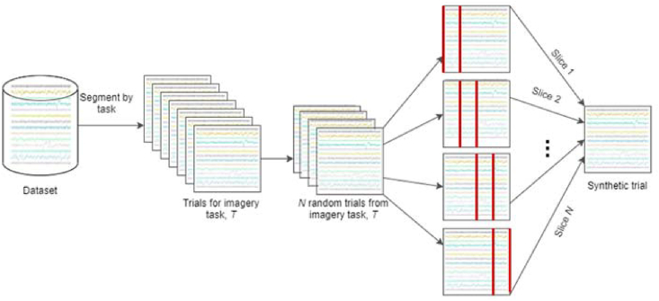
This involves selecting N trials randomly to generate a new trial by recombining roughly equal time slices from all selected trials. We set N to be 5 and combine roughly equal time slices from the 5 trials, for a baseline. N was varied and like AVG, we noticed no significant increase in performance. Figure 2 depicts the process of data generation via recombination of time slices. Recombining slices of trials generates unique trials, which take on patterns from across the originating trials.

Figure 2.

Schematic depicting trial generation by recombining roughly equal time slices of N randomly selected trials.

3.2.3. Recombination of frequency slices (RF)

For recombination in frequency, first, the time-frequency representations of all trials are generated using the short time Fourier transform (STFT). N trials are then randomly selected and roughly equal frequency slices of the trials are combined to generate a new trial. After recombination in frequency domain, the inverse STFT is applied to get the time series representation of all generated trials. N was set to 5 for a baseline and like the previous two approaches, we noticed no significant increase in performance with varied number of recombination trials. Figure 3 depicts the process of data generation via recombination of frequency slices.

Figure 3.

Schematic depicting trial generation by recombining roughly equal frequency slices of N randomly selected trials.

3.2.4. Noise addition (NS)

This approach involves adding random Gaussian noise, generated based on the statistical properties of the data. First, the mean of trials of the class for which trials are generated is calculated. Afterwards, Gaussian noise is generated with zero mean and standard deviation equal to the class mean. The generated noise is then added to randomly selected trials to generate artificial frames. Figure 4 depicts the process of data generation via Gaussian noise addition. The simplistic approach retains the original characteristic of the wave form, while generating trials with slightly different numerical values.

Figure 4.

Schematic depicting trial generation by adding noise to N randomly selected trials.

3.2.5. Cropping (CPS)

Crops were generated, on the data, with a sliding window of length, wlen = 0.5 and overlap = 50%, from start to the end of the trial. Each trial in the training set was broken down into crops of length wlen and crops originating from the same trial were assigned the same label. For testing, prediction scores were generated on crops originating from a test trial, after which the predictions were averaged and the trial was assigned the class with the highest mean score. The number of crops per trial generated is represented by the formula:

$$\frac{’\left(\left(\mathit{trial}\mathit{length}\ast \mathit{sampling}\mathit{rate}\right)-\mathit{crop}\mathit{size}\right)’}{\left(1-n\_\mathit{overlap}\right)\ast \mathit{crop}\_\mathit{size}}+1$$ (1)

where

crop size = wlen ∗ sampling rate = 0.5 ∗ 200 = 60

Number of crops = floor [((1 ∗ 200) - 100)/((1-0.5) ∗ 100)] + 1

= floor(2) + 1 = 2 + 1 = 3

For instance, to generate crops of wlen = 0.5, with n overlap = 50% on dataset II, having trial length = 1 s and 200Hz sampling rate, the number of crops generated is 3. This yields 3 times more data on dataset II. Figure 5 depicts the cropping process. Using crops not only generates more training instances but could allow for learning task-specific patterns in a time window.

Figure 5.

Schematic depicting the cropping process.

3.2.6. Variational autoencoder (VAE)

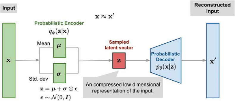
A conditional variational autoencoder was used to learn the distribution of the data and to generate artificial trials based on real ones. The VAE [50] consists of the encoder and the decoder, just as in the case of an autoencoder. In the typical encoder-decoder combination of an autoencoder, the encoder learns a representation of the data and encodes it, by giving a lower-dimensional representation. The decoder, on the other hand, takes the encoded representation and aims to reconstruct the signal back to its original form, thereby decoding the representation. With a VAE, the autoencoder does not simply learn a function that maps the input to a compressed form and back to its original form. Rather, it learns the parameters of the probability distribution describing the data. The representation learned is, therefore, constrained, based on the mean and standard deviation of the data. We conditioned the learning by merging the labels with the trials, during the learning process. The loss function of the VAE was a summed loss function, consisting of the Kullback-Leibler (KL) divergence [51] and mean square reconstruction loss. We applied KL cost annealing [52], training the VAE on the reconstruction loss only for the first 40 epochs and gradually increasing the weight of the KL loss component over the next 20 epochs. The VAE architecture comprises convolutional layers and is seen in Tables A1 and A2 of the appendix. The original training set of the VAE was oversampled as that yielded better losses and training stability. Training was done for 300 epochs with a batch size of 32 and the Adam optimizer was used in the VAE and across all neural networks in this study. Figure 6 below shows the VAE learning process. The VAE differs from other methods given its sophisticated approach of learning the distribution of the real data and before generating synthetic ones.

Figure 6.

Illustration of the learning process of a VAE [53].

3.3. Data evaluation

The quality of the generated data was evaluated using four criteria, namely:

• iAccuracy of prediction using the augmented set as against no augmentation.
• iiFr'echet inception distance (FID).
• iiiTSNE plots of both real and synthetic trials.
• ivTopographic head plots of both real and synthetic trials.

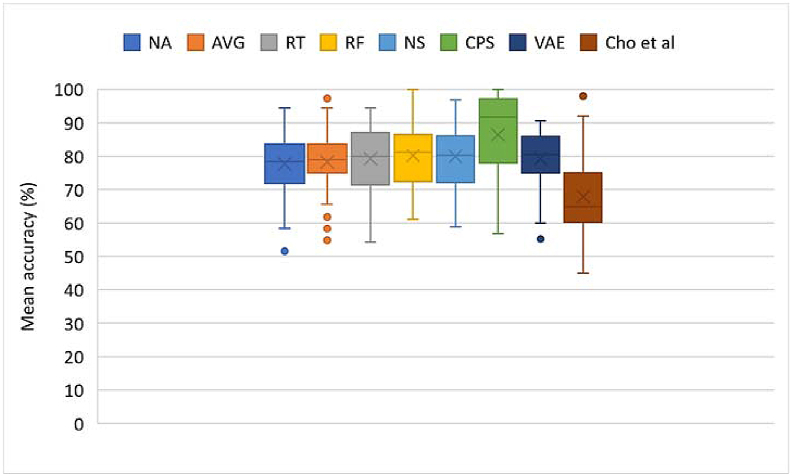
For accuracy evaluation, classification was done using a CNN - the Deep Net, with an architecture inspired by Schirrmeister et al.‘s work [32]. The structure of the network is seen in Table A3 of the appendix. In training the classifier, the already partitioned training set was used with and without augmentation across the mentioned techniques, with the classifier being trained for 50 epochs and with a batch size of 32. As earlier stated, the baseline approach for augmentation was to generate equal number of samples as the number of available trials for each subject and session. Using more augmentation samples yielded no significant improvement. Hence, the baseline was used for comparison across methods. Mean accuracies are shown in Figures 6 and 10 for datasets I and II, respectively.

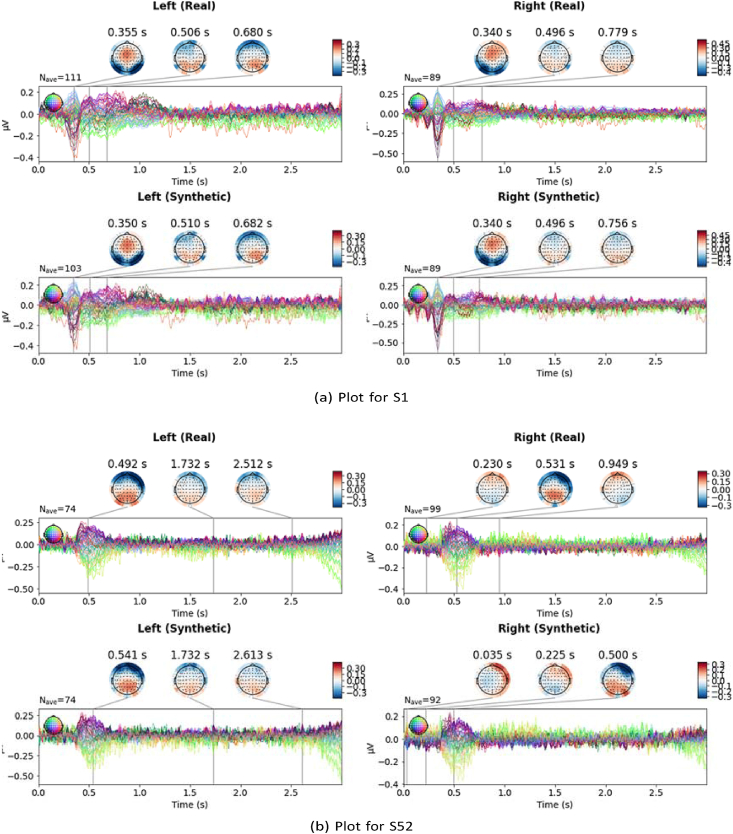
Figure 10.

Topographic plots of subjects of dataset I showing real and synthetic signal characteristics. Plots are shown for subjects (a) S01 and (b) S52, for both left and right classes, using AVG. The reader is referred to the electronic copy for better viewing.

The FID [54] calculates the distance between feature vectors calculated for real and generated samples. It measures how similar they are, in statistical terms, based on the features of the trials calculated using the Inception v3 model [55]. Lower scores show closeness or similarities in properties, being correlated with higher quality data, while larger scores show a greater dissimilarity. The FID on two datasets that are the same is 0. For each augmentation approach, we computed FID values compared with the original data and compare for similarities in distribution due to lower FID scores. FID values are shown in Figures 7 and 11 for datasets I and II, respectively.

Figure 7.

Summary plot of accuracies across all methods for dataset I. NA – No augmentation; AVG – Averaging; RT – Recombination in time; RF – Recombination in frequency; NS – Noise addition; CPS – Crops; VAE – VAE. Crosses and horizontal markers depict the mean and median, respectively.

Figure 11.

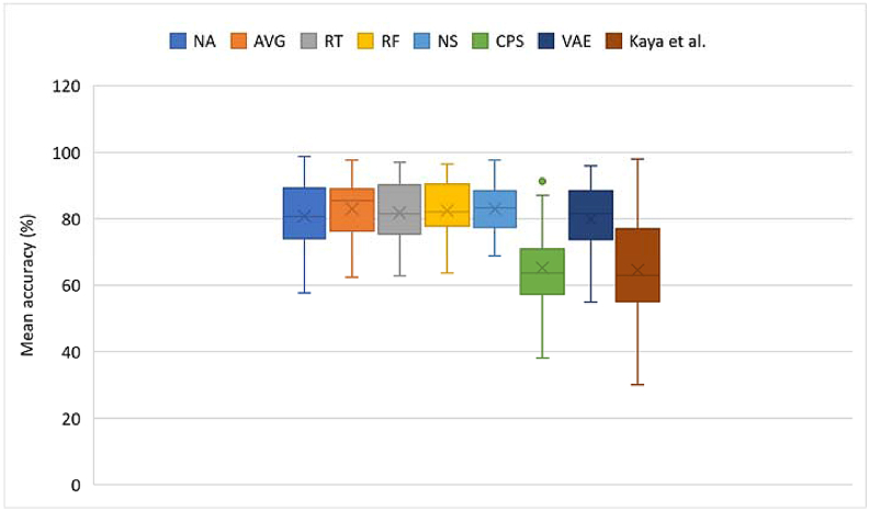
Summary plot of accuracies across all methods for dataset II. NA – No augmentation; AVG – Averaging; RT – Recombination in time; RF – Recombination in frequency; NS – Noise addition; CPS – Crops; VAE – VAE. Crosses and horizontal markers depict the mean and median, respectively.

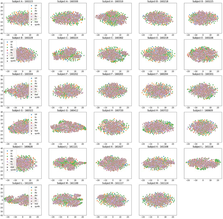
The t-SNE visualization [56] is a dimension-reduced plot of the data. The TSNE procedure compresses an n-dimensional sample into two-dimensions and the plot of the 2-d representations of samples shows how the samples are clustered together. Similarities between well generated and real datasets would be observed by similar clustering and shapes. For each augmentation approach, we generated t-SNE plots to show clustering of original versus synthetic data for all classes. Sample plots for AVG are presented in Figures 8 and 12 for datasets I and II, respectively.

Figure 8.

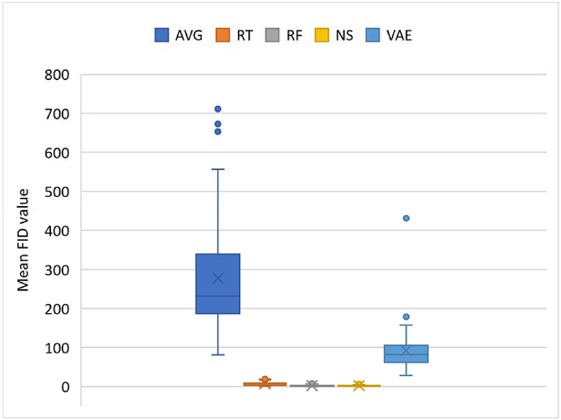
Summary plot of FID values across all methods. AVG – Averaging; RT – Recombination in time; RF – Recombination in frequency; NS – Noise addition; VAE – VAE. CPS is excluded since no new data is calculated and the resulting data form is not of the same dimension as the original trial. Crosses and horizontal markers depict the mean and median, respectively.

Figure 12.

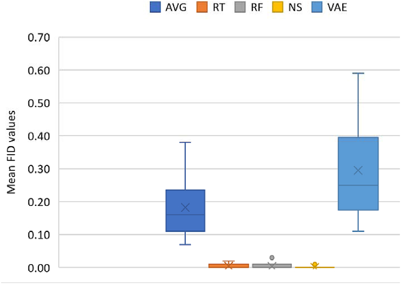
Summary plot of FID values across all methods. AVG – Averaging; RT – Recombination in time; RF – Recombination in frequency; NS – Noise addition; VAE – VAE. CPS is excluded since no new data is calculated and the resulting data form is not of the same dimension as the original trial. Crosses and horizontal markers depict the mean and median, respectively.

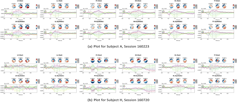
Topographic head plots of evoked responses of both real and synthetic trials were generated, showing brain activity over the course of the trial. It is expected that generated trials would show similar evoked response patterns. This was noticed across the head plots, giving a consistent pattern of events, as expected. Sample plots for datasets I and II are seen in Figures 9 and 13, respectively.

Figure 9.

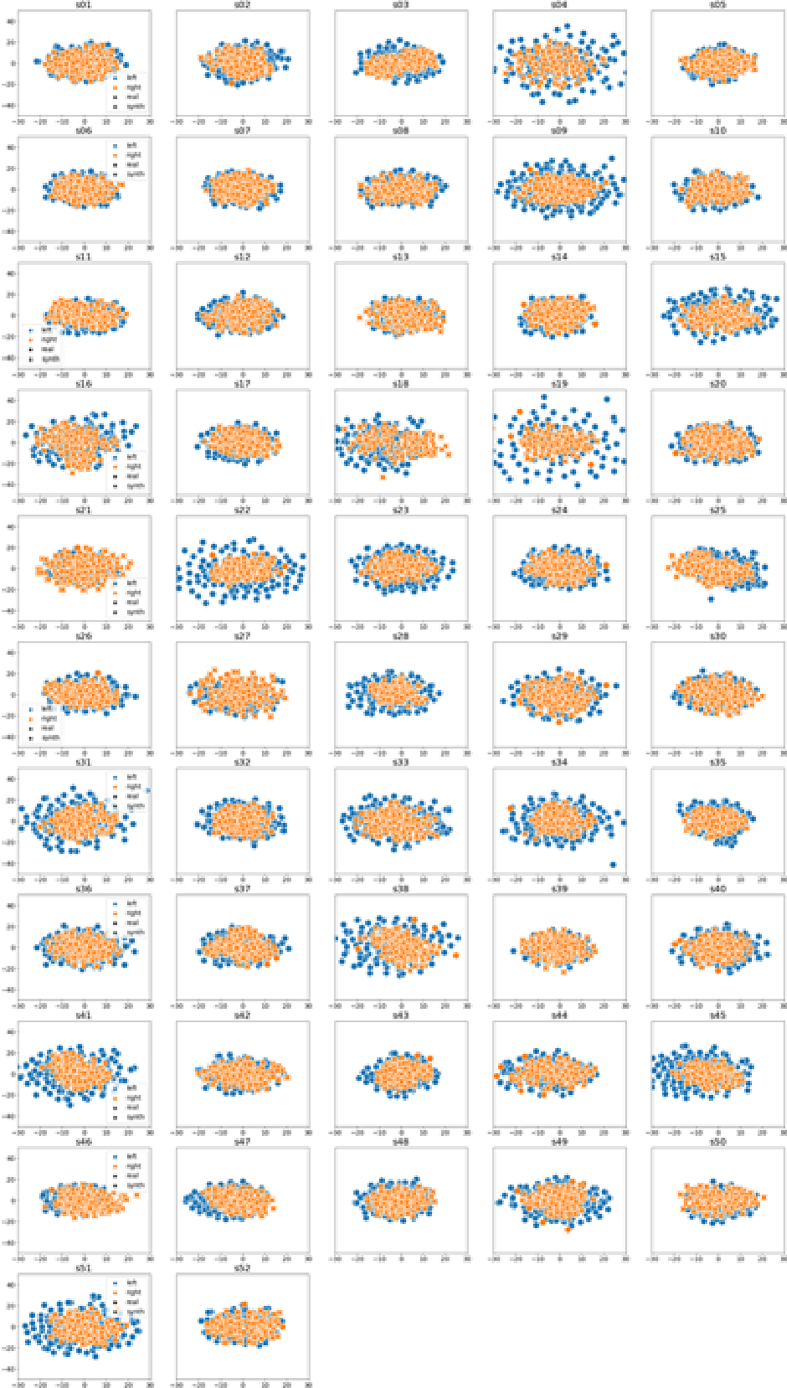
TSNE plots across all 52 subjects of dataset I using AVG augmentation. Real and synthetic (synth) data are plotted as circles and crosses, respectively. Left and right classes are denoted by blue and red colours, respectively. The reader is referred to the electronic copy for better viewing.

Figure 13.

TSNE plot across all subjects and sessions using AVG augmentation. Real and synthetic (synth) data are plotted as circles and crosses, respectively. The reader is referred to the electronic copy for better viewing.

4. Results and discussion

In this section, we present the results of our analyses on the two datasets. The accuracies show how well, a model distinguishes the classes, with and without augmentation; the FID shows the degree of divergence between the synthesized and real data; the TSNE plot shows how real and synthetic trials for all tasks are clustered; and the topographic head plot shows signal characteristics and power across the trial period. For comparisons across methods, p-values were computed using repeated measures one-way analysis of variance (ANOVA) and the Bonferroni-corrected alpha value was set at 7.14E-03.

4.1. Accuracies of classification for Dataset I

Summaries of resulting accuracies are shown in Figure 7 and p-values computed are shown in Table 1. Initial comparison was made for varied number of epochs for generation and varied number of augmentation samples. There was, however, no significant change in results with higher number of generation epochs or augmentation samples. So, equal number of augmentation trials as real trials were generated across subjects and/or sessions for both datasets.

• IAll augmentation methods yielded increases in decoding accuracy

• Compared with no augmentation, all augmentation techniques yielded higher (78.30–86.51 > 77.73) mean accuracies. Though, all p-values except for CPS do not show significance (all p-values > α = 7.14E-03), the increments do show that slight improvements are achievable using these techniques.

• IIMost significant increases were seen using CPS

• The augmentation techniques yielding the most increases on Dataset I were CPS and frequency recombination. RF yielded a higher mean accuracy (80.24 > 77.73) than NA, though not statistically significant (1.09E-01 > α = 7.14E-03). CPS, on the other hand, yielded a higher mean accuracy (86.51 > 77.73), with statistical significance (1.14E-04 < α = 7.14E-03). Model performances improved across 75% of subjects, with up to 12% increase in mean accuracy and most individual increases of 3–30 %, using CPS. In some cases, percentage increases were slightly above 50%. This shows how cropping improved model performances on the dataset. The crops of window length 0.5 (1500 ms) with 50% overlap yielded 3 times more data for each subject, providing smaller windows of data, with certain characteristics that may be peculiar to similar window lengths across trials of the same class. Based on this, the model can learn window-specific features across trials of the same class.

• IIIAll methods significantly outperformed results reported by authors of the dataset

• In comparison with results reported by the original authors [47], all methods, with and without augmentation, gave superior performance with statistical significance (all p-values < α = 7.14E-03). Our approaches significantly differ from the authors' due to the pre-processing, the use of CNNs for classification, rather than traditional machine learning algorithms, and augmentation. Results show better performances following our approaches, as compared to the original authors', meaning that our approaches are preferred.

Table 1.

p-values for comparisons across all methods - Dataset I α = 5E-02; Bonferroni-corrected α with 7 tests = 7.14E-03. Bold values show significance in mean differences.

	NA	AVG	RT	RF	NS	CPS	VAE
AVG	7.20E-01	-	-	-	-	-	-
RT	4.01E-01	5.33E-01	-	-	-	-	-
RF	1.09E-01	2.23E-01	6.13E-01	-	-	-	-
NS	1.81E-01	3.07E-01	7.07E-01	8.97E-01	-	-	-
CPS	1.14E-04	2.05E-04	5.32E-04	5.46E-03	3.47E-03	-	-
VAE	3.15E-01	5.24E-01	9.99E-01	5.24E-01	6.64E-01	2.30E-03	-
Cho et al.	1.40E-05	9.44E-07	2.26E-06	1.59E-09	5.36E-07	6.83E-10	6.96E-07

4.2. FID values for Dataset I

A summary of resulting FID values is shown in Figure 8. FID for all methods were calculated based on the real and synthetic data. So, values were only generated for augmentation techniques yielding trials with dimensions like the original data. CPS was excluded, since crops give smaller dimensions compared to the original data. Moreover, crops are not generated by modifying the values of the original data in any way. Lower FID values are usually preferred, as they show lower divergence, in terms of the distribution, from the real data. NS yielded the least FID. RF and RT also yielded low FID values. FIDs of the VAE and averaging are quite high compared to the others. The low FID of NS shows that the perturbations were not too severe to distort the signals. A recommendation would be to explore RF and NS, as these yielded similar values in terms of accuracy improvements and low FIDs.

4.3. TSNE plots for Dataset I

Figure 9 shows the TSNE plot of real and synthetic data across all subjects in the dataset, using AVG. TSNE plots are helpful in showing how samples are clustered, based on inherent characteristics of the data. Closely clustered points would infer that such points have similar characteristics and so, it is expected that data for the same class, either real or synthetic, would be clustered together, if the augmentation is done well and if the resulting data is not too divergent from the real. Data points are shown to be well clustered with overlaps between real and synthetic data for left and right class labels. The overlaps show similarities between the real and synthetic data. A similar plot for Dataset II is presented in Section 4.7.

4.4. Topographic head plots for Dataset I

The topographic head plots are plots of the evoked response for each class, for both real and synthetic data. The evoked responses are generated by averaging trials, for each class. The plots in Figure 10 show that the characteristics of the synthetic signals are not widely different from those of the real signals. Similar characteristics, in terms of the peaks, are seen across time points of the experiment. With S01, peaks in signals, for the left class, are observed at about 355 ms, 506 ms and 680 ms for the real trial. For the synthetic trial, as well, peaks are observed at 350ms, 510 ms and 682 ms. Similarly, for the right class, we see peaks around 340 ms, 496ms, 756 ms and 779 ms, for both real and synthetic data. These time points are close, showing that the augmentation did not significantly change the observed peaks in evoked responses, across classes for the subjects. With S52, there is a slight variation, though not too wide. A similar plot for dataset II is presented in Section 4.8.

4.5. Accuracies of classification for Dataset II

Summaries of resulting accuracies and computed p-values are shown in Figure 11 and Table 2, respectively. As with dataset I, initial comparisons were done for varied number of generation epochs and augmentation samples. However, no significant change in results was noticed and so, equal number of augmentation trials as real trials were generated across subjects and/or sessions in the dataset.

• IMost augmentation methods yielded increases in decoding accuracy

• Compared with no augmentation, all augmentation techniques, except CPS and the VAE yielded higher (81.74–83.01 > 80.73) mean accuracies. Though, all p-values do not show significant increases (p-values > α = 7.14E- 03), the increments do show that slight improvements are achievable using these techniques.

• IIAll methods, except CPS, significantly outperformed results reported by authors of the dataset

• In comparison with results reported by the original authors [48], all methods, except CPS, gave superior performance with statistical significance (p-values < α = 7.14E-03). As with dataset I, our approaches differ from the authors' due to the pre-processing, the use of CNNs and augmentation.

• IIIResults significantly worsened using CPS, inferred to be due to the trial length

• CPS and VAE yielded lesser mean accuracies than without augmentation (65.17, 79.92 < 80.73), with the decrease from the VAE being statistically insignificant (4.17E-01 ≥ α = 7.14E-03). However, the decrease resulting from the crops is significant (1.37E-10 < α = 7.14E-03), with 93% of subjects having decreases in individual performance, resulting in a 20% total decrease in mean accuracy. We varied the parameters, such as the window length and overlap, for generating the crops but our variation of the parameters, particularly in Dataset II, did not yield performances better than without augmentation. In the comparison of the CPS approach across both datasets, we conclude that CPS might be more suitable with longer trials than shorter ones. The trial length of Dataset I – 3 s - is 3 times more than that of Dataset II – 1 s. The cropped window length for Dataset I covers 1500ms, whereas that of Dataset II covers 600ms. It may be inferred that the 1500ms window length is sufficient to contain discriminatory patterns over the imagery period, as compared to 600ms. Typical reactionary times have been placed at between 200-500ms [56], which is one reason why a longer window length may be more appropriate, since it would, more consistently, capture key signal changes over the course of the task. The significant worsening of results in Dataset II shows the length of trials should be considered before using CPS, as trials of length greater than 1 s might be more suitable than shorter trials when applying CPS.

Table 2.

p-values for comparisons across all methods - Dataset II α = 5E-02; Bonferroni-corrected α with 7 tests = 7.14E-03. Bold values show significance in mean differences.

	NA	AVG	RT	RF	NS	CPS	VAE
AVG	4.74E-02	-	-	-	-	-	-
RT	2.60E-01	2.22E-01	-	-	-	-	-
RF	6.70E-02	4.81E-01	4.66E-01	-	-	-	-
NS	2.27E-02	9.99E-01	1.24E-01	4.73E-01	-	-	-
CPS	1.37E-10	8.57E-12	8.81E-11	1.79E-12	1.46E-13	-	-
VAE	4.17E-01	4.80E-03	1.05E-01	1.35E-03	4.26E-03	4.70E-09	-
Kaya et al.	1.18E-06	4.69E-06	2.60E-06	1.08E-06	9.01E-07	7.76E-01	1.86E-10

4.6. FID values for Dataset II

A summary of resulting FID values is shown in Figure 12. FID for all methods were calculated based on the real and synthetic data. As with the first dataset, FID values were not computed for CPS, since crops give smaller dimensions compared to the original data.

Since lower FID values are preferred, NS, RF and RT yielded the least FIDs, followed by AVG and VAE. Just as with the first dataset, the low FID of NS shows that perturbations were not too severe to distort the signals. Also, a recommendation would be to explore RF, NS and RT, as these yielded low FIDs and improvements in accuracies.

4.7. TSNE plots for Dataset II

TSNE plots for all 12 subjects A-M (excluding D) are shown in Figure 13. The 6 classes of motor imageries are left hand (LH), right hand (RH), left leg (LL), right leg (RL), tongue (TT), passive mode of inactivity (PV). The 6 classes are denoted with the following colours: blue (LH), orange (LL), green (PV), red (RH), purple (RL) and brown (TT). Real and synthetic data points are denoted with circles and crosses, respectively. The data points are shown to be well clustered with overlaps between real and synthetic data for left and right class labels. The overlaps show similarities between the real and synthetic data. TSNE plots of AVG show much finer clustering, compared with other techniques, where there the plots show greater dispersion in the data.

4.8. Topographic head plots for Dataset II

The topographic head plots of the evoked response for each class, for both real and synthetic data are presented in Figure 14, for dataset II. As seen with dataset I, the plots also show similar characteristics between synthetic and real trials. Similar characteristics, in terms of the peaks, are seen across time points of the experiment. With the plot for Subject A (Session 160223), peaks in signals are observed at about 235 ms, 360 ms, 425 ms and 435 ms, in the evoked response plot for the left-hand class, for real and synthetic trials. This same pattern is seen for all 6 classes. Also, for Subject H (Session 160720), similarities in peaks are seen for the tongue imagery, with peaks noticed at 225 ms, 330 ms, 425 ms and 430 ms, for the real and synthetic data. These similarities in peaks are also seen across other imageries. In some cases, slight differences, between observed peaks in real and synthetic data, are seen. However, these changes are not so significant, showing that signals were not undesirably distorted.

Figure 14.

Topographic plots of subjects of dataset II showing real and synthetic signal characteristics, for 6 classes, using AVG. Plots are shown for subjects (a) A – Session 160223 and (b) H – Session 160720. The reader is referred to the electronic copy for better viewing.

4.9. Timings for data generation across all methods

In scenarios where computation time might be a factor to be considered, techniques with less computation time would be desired. Table 3 shows the time taken for data generation, across all methods. Cropping took the least time and might be the preferred augmentation method, where the trial length is also suitable. Compared with others, VAE is seen to be the most computationally expensive, due to the need to train the networks.

Table 3.

Table of timings for data augmentation techniques. Time (in secs) to generate 1000 trials. CPS is for window length = 0.5 and 50% overlap. Times were generated using Kaggle GPU - NVIDIA TESLA P100. CPS took the least time, as shown boldened.

	AVG	RT	RF	NS	CPS	VAE
Dataset I	1.83	0.85	88.52	4.17	0.05	1022.35
Dataset II	0.08	0.10	19.00	0.15	0.02	168.16

4.10. Comparisons with other works

Some recent works exploring data augmentation in motor imagery decoding include works by Freer and Yang [57], K. Zhang et al. [58] Z. Zhang et al. [28] and Dai et al. [33]. In all of these works, only a few augmentation techniques were explored. Freer and Yang [57] applied 5 methods for comparisons. Also, much of their augmentation efforts were toward handling data imbalances, which we handled by oversampling, and not exploring in detail the effect of augmentation across different datasets. K. Zhang et al. [58] also explored 3 augmentation methods. There augmentation was based on spectograms alone and no experimentation was done with the raw data. So also, Z. Zhang et al. [28] and Dai et al. [33] only made use of the empirical mode decomposition (EMD) and time- frequency recombination, respectively. These recent works have limited their exploration to only a few augmentation techniques and have mostly used the BCI competition datasets [29]. These contrast greatly with our work where we have used more augmentation techniques across two datasets of varying trial lengths, showing statistically which methods tend to provide more significant results compared with others

5. Conclusion

In this comparative study, we presented our findings on the use of different data augmentation techniques for motor imagery decoding, using neural networks. We compared a no-augmentation approach with six different augmentation techniques, which can be applied in generating synthetic trials for enhancing decoding performance. The six techniques include: averaging of trials, recombination in time, recombination in frequency, noise addition, cropping and the use of a variational autoencoder (VAE). These techniques range from simple ones (AVG, RT, RF and NS) to more computationally intensive ones, such as the training of the VAE for the augmentation. Our results from applying these techniques, are presented across two public datasets, to investigate these techniques on different datasets of different trial lengths. Time taken for data generation across all techniques is also shown.

Our findings generally show that these techniques offer improvements in performance compared to an un-augmented approach. Across both datasets, noise addition and recombination in frequency seemed to improve decoding performance, with both techniques yielding mean accuracies ≥ 80% on both datasets, albeit not significantly. All techniques gave some form of improvement on both datasets, except for the VAE and cropping, which gave reduced performances on dataset II. The drastic difference in results obtained with cropping on both datasets, implies that the trial length needs to be considered, when applying cropping.

In future, we can consider other techniques, such as the use of a robust lightweight generative adversarial network (GAN), that can learn the data distribution with a smaller number of samples, as are available in motor imagery experiments. GANs have become increasingly popular for data generation and several modifications to the original GAN have been proposed, for different tasks [59, 60, 61, 62].

Noise addition must be done carefully to avoid overly perturbing the data and distorting it. Using the mean and standard deviation for generating Gaussian noise is not recommended, due to the non-stationarity of the signal. We chose to add noise with zero mean and standard deviation equal to the mean of trials for a task. This preserves the data and avoids introducing impurities, which will adversely affect learning. Another approach to noise addition could be performing the perturbations in the frequency space, as the signals are more stationary in that case. In future, we could also investigate noise addition in the frequency domain for comparison with noise addition in time.

A wider gap or variation in performance across the datasets is seen in CPS, as compared with other methods. However, with the other simpler methods, there is less variation, which we infer to be because the full length of trials is used for other methods. Also, parameters for the generation of crops should be selected to achieve optimal crops containing useful information for the learning. Another approach to cropping could involve filtering crops temporally. So, only certain portions of the trial are used. In choosing the most relevant region, a good choice might be 500–2500 ms for the 3-second-long trial or 100–900 ms for the 1-second-long trial. The purpose of crop filtering would be to discard, as much as possible, crops not significantly contributing to the decoding process. Since there exist latencies in subject reactionary times for the performance of the imagery task, filtering out crops of earlier times will reduce the amount of noise resulting from including non-discriminatory crop regions. In future, we could perform correlation analyses on the crops to determine, which ones contain the most significant amount of information. With this, an empirical optimal time range can be selected, though, this may vary across subjects.

In conclusion, we recommend using NS or RT, for quick augmentation and crops for trial lengths greater than 1 s. Where computational power is not a constraint, VAEs could also be explored. In future, we could also use a hybrid approach, by combining more than one augmentation techniques.

Declarations

Author contribution statement

Olawunmi George: Conceived and designed the experiments; Performed the experiments; Analyzed and interpreted the data; Contributed reagents, materials, analysis tools or data; Wrote the paper.

Roger Smith: Contributed reagents, materials, analysis tools or data; Wrote the paper.

Praveen Madiraju: Contributed reagents, materials, analysis tools or data; Wrote the paper.

Nasim Yahyasoltani: Contributed reagents, materials, analysis tools or data; Wrote the paper.

Sheikh Iqbal Ahamed: Contributed reagents, materials, analysis tools or data; Wrote the paper.

Funding statement

This work is partially supported by a number of Grants of Ubicomp Lab, Marquette University, USA [10.13039/100012793].

Data availability statement

Data associated with this study has been deposited at (https://www.nature.com/articles/sdata2018211) and (https://www.ncbi.nlm.nih.gov/pmc/articles/PMC5493744/).

Declaration of interests statement

The authors declare no conflict of interest.

Additional information

No additional information is available for this paper.

Appendix A. Structure of networks

Outputs and dimensions are shown for Dataset I only.

Table A.1.

VAE encoder architecture. trial dimension = (64 ∗ 1536); n nodes 1 = product (trial dimension) = 98304; kernel size 1 = (1, floor (2 ∗ trial dimension [1]/96)) = (1, 32); kernel size 2 = (trial dimension [0], 1) = (64, 1); strides = (1, max (floor (trial dimension [1]/96), 4)) = (1, 16).

Layer Type	Filters	Kernel size	Strides	Output	Connected to
Input 1	-	-	-	(None, 2)	-
Embedding 1	-	-	-	(None, 2, 10)	Input 1
Flatten 1	-	-	-	(None, 20)	Embedding 1
Dense 1	5	-	-	(None, 5)	Flatten 1
Dense 2	n nodes 1	-	-	(None, 98304)	Dense 1
Reshape 1	-	-	-	(None, 64, 1536, 1)	Dense 2
Input 2	-	-	-	(None, 64, 1536, 1)	-
Concatenate 1	-	-	-	(None, 64, 1536, 2)	Input 2 Reshape 1
Conv 1	16	kernel size 1	strides	(None, 64, 95, 16)	Concatenate 1
LeakyReLU 1	-	-	-	(None, 64, 95, 16)	Conv 1
Conv 2	32	kernel size 2	-	(None, 1, 95, 32)	LeakyReLU 1
LeakyReLU 2	-	-	-	(None, 1, 95, 32)	Conv 2
Flatten 2	-	-	-	(None, 3040)	LeakyReLU 2
Dense 3	16	-	-	(None, 16)	Flatten 2
Dense 4	10	-	-	(None, 10)	Dense 3
Dense 5	10	-	-	(None, 10)	Dense 3
Sampling 1	-	-	-	(None, 10)	Dense 4 Dense 5

Table A.2.

VAE decoder architecture. trial dimension = (64 ∗ 1536); kernel size 1 = (trial dimension [0], 1) = (64, 1); kernel size 2 = (1, floor (2 ∗ trial dimension [1]/96)) = (1, 32) strides = (1, max (floor (trial dimension [1]/96), 4)) = (1, 16) ∗ add padding to retain previous dimension.

Layer Type	Filters	Kernel size	Strides	Output	Connected to
Input 1	-	-	-	(None, 10)	-
Dense 1	3040	-	-	(None, 3040)	Input 1
LeakyReLU 1	-	-	-	(None, 3040)	Dense 1
Reshape 1	-	-	-	(None, 1, 95, 32)	LeakyReLU 1
ConvTranspose 1	64	kernel size 1	-	(None, 64, 95, 64)	Reshape 1
LeakyReLU 2	-	-	-	(None, 64, 95, 64)	ConvTranspose 1
ConvTranspose 2	32	kernel size 2	strides	(None, 64, 1536, 32)	LeakyReLU 2
LeakyReLU 3	-	-	-	(None, 64, 1536, 32)	ConvTranspose 2
ConvTranspose 3 ∗	1	7	-	(None, 64, 1536, 1)	LeakyReLU 3
LeakyReLU 4	-	-	-	(None, 64, 1536, 1)	ConvTranspose 3

Table A.3.

Structure of the Deep Net classifier trial dimension = (64 ∗ 1536); kernel size = (1, floor ((5 ∗ trial dimension [1])/(256 ∗ 1))) = (1,30); pool size = (1, max (floor ((trial dimension [1] ∗ 2)/(256 ∗ 4)), 2)) = (1, 3); strides= (1, max (floor ((trial dimension [1] ∗ 2)/(256 ∗ 4)), 2)) = (1, 3).

Layer Type	Filters	Kernel size	Pool size	Strides	Dropout rate	Output
Input	-	-	-	-	-	(None, 1, 64, 1536)
Conv	25	(1, 30)	-	-	-	(None, 25, 64, 1507)
Conv	25	(1, 30)	-	-	-	(None, 25, 1, 1507)
Batch Normalization	-	-	-	-	-	(None, 25, 1, 1507)
Activation (SELU)	-	-	-	-	-	(None, 25, 1, 1507)
Average pooling	-	-	(1, 3)	(1, 3)	-	(None, 25, 1, 502)
Dropout	-	-	-	-	0.4	(None, 25, 1, 502)
Conv	50	(1, 30)	-	-	-	(None, 50, 1, 473)
Batch Normalization	-	-	-	-	-	(None, 50, 1, 473)
Activation (SELU)	-	-	-	-	-	(None, 50, 1, 473)
Average pooling	-	-	(1, 3)	(1, 3)	-	(None, 50, 1, 157)
Dropout	-	-	-	-	0.4	(None, 50, 1, 157)
Conv	100	(1, 30)	-	-	-	(None, 100, 1, 128)
Batch Normalization	-	-	-	-	-	(None, 100, 1, 128)
Activation (SELU)	-	-	-	-	-	(None, 100, 1, 128)
Average pooling	-	-	(1, 3)	(1, 3)	-	(None, 100, 1, 42)
Dropout	-	-	-	-	0.4	(None, 100, 1, 42)
Conv	200	(1, 30)	-	-	-	(None, 200, 1, 13)
Batch Normalization	-	-	-	-	-	(None, 200, 1, 13)
Activation (SELU)	-	-	-	-	-	(None, 200, 1, 13)
Max pooling	-	-	(1, 3)	(1, 3)	-	(None, 200, 1, 4)
Dropout	-	-	-	-	0.4	(None, 200, 1, 4)
Flatten	-	-	-	-	-	(None, 800)
Dense	6	-	-	-	-	(None, 2)
Activation (Softmax)	-	-	-	-	-	(None, 2)

References

- 1.L. Huang, G. van Luijtelaar, Brain Computer Interface for Epilepsy Treatment, Brain-Computer Interface Systems-Recent Progress and Future Prospects.
- 2.Tzallas A.T., Giannakeas N., Zoulis K.N., Tsipouras M.G., Glavas E., Tzimourta K.D., Astrakas L.G., Konitsiotis S. 2017-June. 2017. (EEG Classification and Short-Term Epilepsy Prognosis Using Brain Computer Interface Software). [Google Scholar]
- 3.J. A. Stevens, M. E. P. Stoykov, Using motor imagery in the rehabilitation of hemiparesis, Arch. Phys. Med. Rehabil. 84. doi: . [DOI] [PubMed]
- 4.de Vries S., Mulder T. 2007. Motor Imagery and Stroke Rehabilitation: A Critical Discussion. [DOI] [PubMed] [Google Scholar]
- 5.Zimmermann-Schlatter A., Schuster C., Puhan M.A., Siekierka E., Steurer J. 2008. Efficacy of Motor Imagery in post-stroke Rehabilitation: A Systematic Review. [DOI] [PMC free article] [PubMed] [Google Scholar]
- 6.R. Dickstein, A. Dunsky, E. Marcovitz, Motor imagery for gait rehabilitation in post-stroke hemiparesis, Phys. Ther. 84. doi:. [PubMed]
- 7.Pfurtscheller G., Müller-Putz G.R., Pfurtscheller J., Rupp R. EEG-based asynchronous bci controls functional electrical stimulation in a tetraplegic patient. EURASIP J. Appl. Signal Process. 2005 [Google Scholar]
- 8.B. A. S. Hasan, J. Q. Gan, Hangman bci: an unsupervised adaptive selfpaced brain-computer interface for playing games, Comput. Biol. Med. 42. doi:. [DOI] [PubMed]
- 9.Soraghan C., Matthews F., Kelly D., Ward T., Markham C., Pearlmutter B.A., Neill R.O. 2006. A Dual-Channel Optical Brain-Computer Interface in a Gaming Environment. [Google Scholar]
- 10.D. Marshall, D. Coyle, S. Wilson, M. Callaghan, Games, gameplay, and bci: the state of the art, IEEE Transactions on Computational Intelligence and AI in Games 5. doi:.
- 11.T. Shi, H. Wang, C. Zhang, Brain computer interface system based on indoor semi-autonomous navigation and motor imagery for unmanned aerial vehicle control, Expert Syst. Appl. 42. doi:.
- 12.Zhuang J., Yin G. 2017. Motion Control of a Four-Wheel-Independent-Drive Electric Vehicle by Motor Imagery EEG Based Bci System. [Google Scholar]
- 13.C. Neuper, M. Wortz, G. Pfurtscheller, Erd/ers Patterns Reflecting Sensorimotor Activation and Deactivation, Event-Related Dynamics of Brain Oscillations 159. [DOI] [PubMed]
- 14.Wolpaw J.R., Birbaumer N., McFarland D.J., Pfurtscheller G., Vaughan T.M. 2002. Brain-computer Interfaces for Communication and Control. [DOI] [PubMed] [Google Scholar]
- 15.D. J. McFarland, J. R. Wolpaw, Brain-computer interfaces for communication and control, Commun. ACM 54. doi:. [DOI] [PMC free article] [PubMed]
- 16.G. Schalk, D. J. McFarland, T. Hinterberger, N. Birbaumer, J. R. Wolpaw, Bci2000: a general-purpose brain-computer interface (bci) system, IEEE (Inst. Electr. Electron. Eng.) Trans. Biomed. Eng. 51. doi:. [DOI] [PubMed]
- 17.J. Decety, Behavioural brain research the neurophysiological basis of motor imagery, Behav. Brain Res. 77. [DOI] [PubMed]
- 18.G. Pfurtscheller, C. Neuper, Motor imagery and direct brain-computer communication, Proc. IEEE 89. doi:.
- 19.Abdelfattah S.M., Abdelrahman G.M., Wang M. 2018-July. 2018. (Augmenting the Size of EEG Datasets Using Generative Adversarial Networks). [Google Scholar]
- 20.I. Ullah, M. Hussain, E. ul Haq Qazi, H. Aboalsamh, An automated system for epilepsy detection using eeg brain signals based on deep learning approach, Expert Syst. Appl. 107. doi:.
- 21.Amin S.U., Alsulaiman M., Muhammad G., Mekhtiche M.A., Hossain M.S. Deep learning for eeg motor imagery classification based on multi-layer cnns feature fusion. Future Generation Computer Systems- The International Journal of Escience. 2019;101:542–554. [Google Scholar]
- 22.Azab A.M., Mihaylova L., Ang K.K., Arvaneh M. Weighted transfer learning for improving motor imagery-based brain-computer interface. IEEE Trans. Neural Syst. Rehabil. Eng. 2019;27:1352–1359. doi: 10.1109/TNSRE.2019.2923315. [DOI] [PubMed] [Google Scholar]
- 23.R. Boostani, B. Graimann, M. H. Moradi, G. Pfurtscheller, A comparison approach toward finding the best feature and classifier in cue-based BCI, Med. Biol. Eng. Comput. 45. doi:. [DOI] [PubMed]
- 24.Choi D., Ryu Y., Lee Y., Lee M. Performance evaluation of a motorimagery-based eeg-brain computer interface using a combined cue with heterogeneous training data in bci-naive subjects. Biomed. Eng. Online. 2011;10:91. doi: 10.1186/1475-925X-10-91. [DOI] [PMC free article] [PubMed] [Google Scholar]
- 25.Ron-Angevin R., Velasco-Alvarez F., Sancha-Ros S., Silva-Sauer L.D. 2011. A Two-Class Self-Paced Bci to Control a Robot in Four Directions. [DOI] [PubMed] [Google Scholar]
- 26.Wang C., Xia B., Li J., Yang W., Xiao D., Velez A.C., Yang H. Vol. 1. 2011. (Motor Imagery Bci-Based Robot Arm System). [Google Scholar]
- 27.F. Velasco-A´lvarez, R. Ron-Angevin, L. da Silva-Sauer, S. Sancha-Ros, Audio-cued motor imagery-based brain-computer interface: navigation through virtual and real environments, Neurocomputing 121. doi:.
- 28.Zhang Z., Duan F., Sole-Casals J., Dinares-Ferran J., Cichocki A., Yang Z., Sun Z. A novel deep learning approach with data augmentation to classify motor imagery signals. IEEE Access. 2019;7:15945–15954. [Google Scholar]
- 29.Competition B. 2003. Bci competition i-iv.http://www.bbci.de/competition/ URL. [Google Scholar]
- 30.Li Y., Zhang X.-R., Zhang B., Lei M.-Y., Cui W.-G., Guo Y.-Z. A channel-projection mixed-scale convolutional neural network for motor imagery eeg decoding. IEEE Trans. Neural Syst. Rehabil. Eng. 2019;27:1170–1180. doi: 10.1109/TNSRE.2019.2915621. [DOI] [PubMed] [Google Scholar]
- 31.Blankertz B. 2008. Bci Competition Iv, 2008; pp. 2–4.http://www.bbci.de/competition/iv/ URL. [Google Scholar]
- 32.R. T. Schirrmeister, J. T. Springenberg, L. D. J. Fiederer, M. Glasstetter, K. Eggensperger, M. Tangermann, F. Hutter, W. Burgard, T. Ball, Deep learning with convolutional neural networks for eeg decoding and visualization, Hum. Brain Mapp. 38. doi:. [DOI] [PMC free article] [PubMed]
- 33.G. Dai, J. Zhou, J. Huang, N. Wang, Hs-cnn: a cnn with hybrid convolution scale for eeg motor imagery classification, J. Neural. Eng. 17. doi:. [DOI] [PubMed]
- 34.Z. Tayeb, J. Fedjaev, N. Ghaboosi, L. R. Christoph, Everding, X. Qu, Y. Wu, G. Cheng, J. Conradt, Validating deep neural networks for online decoding of motor imagery movements from eeg signals, Sensors 19. doi:. [DOI] [PMC free article] [PubMed]
- 35.I. Goodfellow, J. Pouget-Abadie, M. Mirza, B. Xu, D. Warde-Farley, S. Ozair, A. Courville, Y. Bengio, Generative adversarial nets (nips version), Adv. Neural Inf. Process. Syst. 27.
- 36.Odena A., Olah C., Shlens J. Vol. 6. 2017. (Conditional Image Synthesis with Auxiliary Classifier gans). [Google Scholar]
- 37.Wang T.C., Liu M.Y., Zhu J.Y., Tao A., Kautz J., Catanzaro B. 2018. High-resolution Image Synthesis and Semantic Manipulation with Conditional Gans. [Google Scholar]
- 38.Kazeminia S., Baur C., Kuijper A., van Ginneken B., Navab N., Albarqouni S., Mukhopadhyay A. 2020. Gans for Medical Image Analysis, Artificial Intelligence in Medicine. [DOI] [PubMed] [Google Scholar]
- 39.M. Wiese, R. Knobloch, R. Korn, P. Kretschmer, Quant gans: Deep Generation of Financial Time Series, Quant. Finance 20. doi:.
- 40.S. Takahashi, Y. Chen, K. Tanaka-Ishii, Modeling financial time-series with generative adversarial networks, Phys. Stat. Mech. Appl. 527. doi:.
- 41.Zhou X., Pan Z., Hu G., Tang S., Zhao C. Stock market prediction on highfrequency data using generative adversarial nets. Math. Probl Eng. 2018 [Google Scholar]
- 42.Luo Y., Lu B.-L. 2018. EEG Data Augmentation for Emotion Recognition Using a Conditional Wasserstein gan; pp. 2535–2538. [DOI] [PubMed] [Google Scholar]
- 43.Corley I.A., Huang Y. 2018-January. 2018. (Deep EEG Super-resolution: Upsampling EEG Spatial Resolution with Generative Adversarial Networks). [Google Scholar]
- 44.Wang F., Zhong S.H., Peng J., Jiang J., Liu Y. Vol. 10705. LNCS; 2018. (Data Augmentation for EEG-Based Emotion Recognition with Deep Convolutional Neural Networks). [Google Scholar]
- 45.Roy S., Dora S., McCreadie K., Prasad G. 2020. Mieeg-gan: Generating Artificial Motor Imagery Electroencephalography Signals. [Google Scholar]
- 46.T. J. Luo, Y. Fan, L. Chen, G. Guo, C. Zhou, EEG signal reconstruction using a generative adversarial network with wasserstein distance and temporal-spatial-frequency loss, Front. Neuroinf. 14. doi: . [DOI] [PMC free article] [PubMed]
- 47.Cho H., Ahn M., Ahn S., Kwon M., Jun S.C. 2017. EEG Datasets for Motor Imagery Brain-Computer Interface. [DOI] [PMC free article] [PubMed] [Google Scholar]
- 48.M. Kaya, M. K. Binli, E. Ozbay, H. Yanar, Y. Mishchenko, Data descriptor: a large electroencephalographic motor imagery dataset for electroencephalographic brain computer interfaces, Sci. Data 5. doi: . [DOI] [PMC free article] [PubMed]
- 49.M. Jas, D. A. Engemann, Y. Bekhti, F. Raimondo, A. Gramfort, Autoreject: automated artifact rejection for meg and eeg data, Neuroimage 159. doi:. [DOI] [PMC free article] [PubMed]
- 50.Kingma D.P., Welling M. 2014. Auto-encoding Variational Bayes. [Google Scholar]
- 51.T. V. Erven, P. Harr¨emos, R´enyi divergence and kullback-leibler divergence, IEEE Trans. Inf. Theor. 60. doi:.
- 52.Chen X., Kingma D.P., Salimans T., Duan Y., Dhariwal P., Schulman J., Sutskever I., Abbeel P. 2017. Variational Lossy Autoencoder. [Google Scholar]
- 53.Weng L. From Autoencoder to Beta-Vae, lilianweng.github.Io. https://lilianweng.github.io/posts/2018-08-12-vae/ URL.
- 54.Heusel M., Ramsauer H., Unterthiner T., Nessler B., Hochreiter S. Vol. 2017. 2017-December. (Gans Trained by a Two Time-Scale Update Rule Converge to a Local Nash Equilibrium). [Google Scholar]
- 55.Szegedy C., Vanhoucke V., Ioffe S., Shlens J., Wojna Z. 2016-December. 2016. (Rethinking the Inception Architecture for Computer Vision). [Google Scholar]
- 56.L. V. D. Maaten, G. Hinton, Visualizing data using t-sne, J. Mach. Learn. Res. 9.
- 57.Freer D., Yang G.-Z. Data augmentation for self-paced motor imagery classification with c-lstm. J. Neural. Eng. 2020;17(1) doi: 10.1088/1741-2552/ab57c0. [DOI] [PubMed] [Google Scholar]
- 58.Zhang K., Xu G., Han Z., Ma K., Zheng X., Chen L., Duan N., Zhang S. Data augmentation for motor imagery signal classification based on a hybrid neural network. Sensors. 2020;20(16):4485. doi: 10.3390/s20164485. [DOI] [PMC free article] [PubMed] [Google Scholar]
- 59.Mao X., Li Q., Xie H., Lau R.Y., Wang Z., Smolley S.P. Least squares generative adversarial networks. 2017;2017-October doi: 10.1109/TPAMI.2018.2872043. [DOI] [PubMed] [Google Scholar]
- 60.M. Arjovsky, S. Chintala, L. Bottou, Wasserstein gan, arXiv preprint arXiv:1701.07875.
- 61.P. Isola, J. Y. Zhu, T. Zhou, A. A. Efros, Pix2pix-gan, Proceedings - 30th IEEE Conference on Computer Vision and Pattern Recognition, CVPR 2017 2017-Janua.
- 62.Radford A., Metz L., Chintala S. 2016. Unsupervised Representation Learning with Deep Convolutional Generative Adversarial Networks. [Google Scholar]
Associated Data
This section collects any data citations, data availability statements, or supplementary materials included in this article.