

Abstract
Motivation
Local ancestry inference (LAI) is the high resolution prediction of ancestry labels along a DNA sequence. LAI is important in the study of human history and migrations, and it is beginning to play a role in precision medicine applications including ancestry-adjusted genome-wide association studies (GWASs) and polygenic risk scores (PRSs). Existing LAI models do not generalize well between species, chromosomes or even ancestry groups, requiring re-training for each different setting. Furthermore, such methods can lack interpretability, which is an important element in each of these applications.
Results
We present SALAI-Net, a portable statistical LAI method that can be applied on any set of species and ancestries (species-agnostic), requiring only haplotype data and no other biological parameters. Inspired by identity by descent methods, SALAI-Net estimates population labels for each segment of DNA by performing a reference matching approach, which leads to an interpretable and fast technique. We benchmark our models on whole-genome data of humans and we test these models’ ability to generalize to dog breeds when trained on human data. SALAI-Net outperforms previous methods in terms of balanced accuracy, while generalizing between different settings, species and datasets. Moreover, it is up to two orders of magnitude faster and uses considerably less RAM memory than competing methods.
Availability and implementation
We provide an open source implementation and links to publicly available data at github.com/AI-sandbox/SALAI-Net. Data is publicly available as follows: https://www.internationalgenome.org (1000 Genomes), https://www.simonsfoundation.org/simons-genome-diversity-project (Simons Genome Diversity Project), https://www.sanger.ac.uk/resources/downloads/human/hapmap3.html (HapMap), ftp://ngs.sanger.ac.uk/production/hgdp/hgdp_wgs.20190516 (Human Genome Diversity Project) and https://www.ncbi.nlm.nih.gov/bioproject/PRJNA448733 (Canid genomes).
Supplementary information
Supplementary data are available from Bioinformatics online.
1 Introduction
1.1 Genomic data and its applications
Sequencing technology advances are enabling the generation of genome-wide data at rapidly decreasing cost. These genome sequences, combined with modern statistical and computational techniques, are providing a new data-driven paradigm in many areas including population genetics, precision medicine and agriculture. For example, genome-wide data for human individuals are allowing prediction of disease risk through genome-wide association studies (GWASs) and polygenic risk scores (PRS) and allowing for the study of migration and historical events through genomic ancestry analysis. These analyses are not unique to human data, but are also being applied to animals and plants, leading to improvements in farming and agriculture, while providing methods to better understand genetic and phenotypic differences between breeds, cultivars and species. The increase in data availability and in genomic-based applications has created a need for computational tools that are fast, efficient and portable across species and applications.
Genome sequences are composed of four nucleotides, typically represented with the letters: A, T, C and G. While the majority of genomic positions are fixed across individuals of the same species, a small fraction is known to be variable. Most of these positions are single-nucleotide polymorphisms (SNPs) that have two variants or forms, which allows for a binary encoding with a common or majority variant (encoded as a zero) shared among the majority of individuals and a minority or alternative variant (encoded as a one) (Avallone et al., 2020; Ioannidis et al., 2020; Kumar et al., 2020; Maples et al., 2013; Thornton and Bermejo, 2014).
Throughout history human populations across distinct geographical regions have experienced periods of isolation and independent genetic drift along with periods of migration and admixture. This process has resulted in various genetic ancestry clusters (populations) that have slightly different allele frequencies and allele correlations (linkage disequilibrium). While this variation allows us to date and quantify historical migration events, it also makes the development of globally applicable statistical predictive models difficult. For example, a PRS model developed using samples from European populations will, in many cases, perform poorly when applied to African individuals (Martin et al., 2017). Such a lack of generalization across populations leads in turn to disparities in the efficacy of disease risk prediction and drug response adjustment.
Current human population groups are far less isolated from each other and recently admixed individuals are increasingly common. Such genetic admixture occurs when previously largely separated populations come into contact. Genomic sequences from such admixed individuals tend to have a mosaic-like structure with different segments of their genomes originating from different ancestral populations (Supplementary Fig. S1a). Admixture can continue over multiple generations, yielding individuals with DNA from different ancestries and of different lengths. Local ancestry inference (LAI) is a method to identify this mosaic of ancestry segments, allowing ancestry-specific models to be applied to the labeled genomes (Atkinson et al., 2021; Ioannidis et al., 2021; Marnetto et al., 2020).
Other animal and plant species possess genetic variation typically much greater than that observed within humans, making LAI in them possible and important. While variation within wild species typically reflects geography, with more distant groups more different genetically, domesticated animals and plants tend to have genetic substructures reflecting their breeding (artificial selection) by humans. Techniques to characterize the ancestry composition of animals and plants are increasingly used (Flowers et al., 2019; Joukhadar et al., 2017). Some examples include commercial applications of breed analysis in domestic animals such as dogs, cats or horses, or phenotypic prediction in crops. The number of population groups, chromosomes and available SNPs vary widely (from thousands to millions of SNPs) between species and sequencing technologies. Therefore, methods that can easily adapt to widely different settings and can handle potentially long sequences are required if ancestry analysis is to be easily adopted within the genetic analysis of both human and non-humans.
1.2 Introduction to LAI
LAI is the prediction of the ancestral origin for each piece of an individual’s genome. LAI has become increasingly important in the field of genomic data processing (Martin et al., 2017; Raghavan et al., 2015; Thornton and Bermejo, 2014) and its applications range from the study of human migrations and evolution (Avallone et al., 2020; Ioannidis et al., 2020; Padhukasahasram, 2014; Raghavan et al., 2015) to GWAS adjustment (Atkinson et al., 2021) and PRS prediction (Marnetto et al., 2020; Martin et al., 2017; Suarez-Pajes et al., 2021).
Most previous methods for LAI learn a set of parameters [e.g. parameters of graphical models such as Hidden Markov Models (HMMs)] (Price et al., 2009; Sundquist et al., 2008; Tang et al., 2006) or weights of neural networks (Montserrat et al., 2020) tailored to the specific genotypes available within a reference training panel, for a given species, chromosome and set of population groups. Such methods completely fail when faced with SNP loci not seen during training. That is, for example, when seeing genomic positions from different species or even from different chromosomes or genetic positions in the same species. Such lack of generalization is due to the fact that the statistics of the genomic sequences vary greatly across positions on the genome and across species. Therefore, such methods require re-training for each new setting. In this work, we adopt a new framework, which, unlike the usual LAI methods, allows us to perform inference on any species, chromosomes and set of populations, without the need for training a new model. This is accomplished by estimating the ancestry along the sequence by looking at similarities between the input sequence and a reference panel (Supplementary Fig. S1b), without learning any new species or chromosome-specific parameters. We refer to this approach as species-agnostic or setting-agnostic LAI.
In order to perform training or inference with local ancestry methods, a reference panel of sequences from single-ancestry individuals with known ancestry group labels (ground-truth) is required. Such reference information is obtained through self-reported ancestry, prior domain knowledge or unsupervised clustering (Gimbernat-Mayol et al., 2021), and in many cases, validated with additional statistical analyses. While traditional LAI methods can be trained with single-ancestry sequences, recent LAI models have demonstrated training with synthetically generated data (Montserrat et al., 2019; Perera et al., 2022). These synthetic references can be computationally admixed (Karavani et al., 2019), and by tracking which DNA segments are recombined with each other during admixture simulation, high-resolution ancestry labels from (simulated) admixed individuals can be obtained (Gravel, 2012), enabling the production of large synthetic datasets with high resolution ground truth labels. Such simulation of recombination is a common practice when evaluating LAI methods, as obtaining ground-truth admixed genome labels (via sequencing of trios) is costly and time-consuming.
The adopted reference panel matching approach, described in detail in the next section, removes entirely the need for re-training the system for new populations, new species or new chromosomes and for performing simulations of admixed genomes, leading to a faster and less computationally demanding system that is also more accessible, especially for users without the hardware resources and expertise needed to fully train a machine-learning model in an agile and optimal fashion. In fact, by providing pre-trained models, our method only requires that a set of single-ancestry reference panels be provided by the user, no subsequent model training is necessary.
1.3 Previous work
Over the last 15 years, there have been many different approaches to LAI. Some examples include techniques based on HMMs such as SABER (Tang et al., 2006), HAPAA (Sundquist et al., 2008) and HAPMIX (Price et al., 2009). Other examples include LAMP (Sankararaman et al., 2008), which outperforms HMM-based methods and is based on a window-level probability maximization. However, its publicly available implementation is limited in the number of ancestries that can be used. While such methods perform accurately on low-resolution genotype array data, they are not optimized for whole-genome sequencing technologies, which generally lead to extremely large training times that are not possible in practice. More recent methods, such as RFMix (Maples et al., 2013), based on random forests with conditional random fields, provide higher accuracy with more tractable training times on whole genome data. Recently Loter (Dias-Alves et al., 2018), which is based on dynamic optimization, has achieved better accuracy and robustness across different species than previous methods. Finally, LAI-Net (Montserrat et al., 2020), the first neural network-based local ancestry algorithm, has surpassed RFMix accuracy.
Neural networks have become the state of the art in multiple tasks involving sequence modelling across fields and data modalities (Kong et al., 2019; Oord et al., 2016; Ren et al., 2019; Vaswani et al., 2017). These networks model sequences using parametric linear transformations combined with non-linear mappings. The parameters of these models are optimized in an end-to-end fashion for a given loss function. An important building block of many neural networks are convolutions, which are adopted in this work, and are widely used in computer vision (Voulodimos et al., 2018), natural language processing (Oord et al., 2016; Vaswani et al., 2017) and genomic data processing (Mantes et al., 2022; Montserrat et al., 2020; Zaheer et al., 2020). LAI-Net (Montserrat et al., 2020) was the first neural network-based method to perform LAI and it reaches competitive results while providing robustness to missing or noisy data. Despite its accuracy, this model is not species-agnostic and requires re-training for every new setting encountered, which can be computationally demanding, since GPUs are required to properly train the neural network. Similar to RFMix, LAI-Net follows a two-stage approach: an initial classification stage and a smoothing or refinement stage. LAI-Net begins by segmenting the input sequence into non-overlapping windows of 500 SNPs. Next, a different two-layer multi-layer perceptron (MLP) of hidden size 30 is applied to each window to obtain an initial estimation of the ancestry predictions. Then, the smoother stage corrects the errors induced by the MLP classifiers by using information from neighbouring windows through a trained convolutional layer of kernel size 75 with kernel depth and number of kernels equal to the number of population groups. This two-stage design used in LAI-Net and RFMix inspires the architecture used in SALAI-Net, but novel classifiers and smoothing approaches are introduced in order to obtain the desired species-agnostic portability and to remove the need for training and simulation.
Loter (Dias-Alves et al., 2018) is the current state of the art in interpretable species-agnostic LAI. Loter uses a reference panel matching-based approach combined with a dynamic programming decoding (Viterbi-like) to infer the ancestry composition of admixed sequences. By assigning a cost that penalizes over-splitting of the ancestry segments, the optimal sequence of ancestry transitions is found. Moreover, Loter uses a data bagging scheme that makes multiple initial predictions with different hyperparameters and reference panel subsets and then produces the final prediction with a voting ensemble. Our method adopts a different reference panel matching strategy and replaces the dynamic programming by a simple convolution, leading to both faster and more accurate predictions.
2 Materials and methods
2.1 SALAI-Net
We refer to our presented model as SALAI-Net: Species Agnostic LAI Network (Fig. 1). Similarly to previous methods, SALAI-Net follows a two-stage approach: a reference matching layer followed by a smoother layer. The reference matching layer provides window-level initial estimates and the smoother layer improves the initial predictions by exploiting neighbouring window information and smoothing out errors. SALAI-Net is trained in a specific setting and after that it can be used for LAI across any other species, or for any other set of ancestries, without needing retraining or tuning.
Fig. 1.

Diagram of the two main layers of SALAI-Net, followed by an up-sampling layer that repeats each window prediction to match the original sequence length
2.1.1 Reference matching layer
The reference matching layer (Fig. 2) computes initial matching scores between the query sequence (the input admixed sequence) and the reference panel (templates). The proposed layer has few learnable parameters, which is critical to assuring generalization to other species and settings while maintaining accuracy. First, the admixed query sequence and reference panel sequences are split into Nwin non-overlapping windows of size W SNPs. Then, a cosine similarity score between the query sequence and each of the Nrefs reference sequences is computed at every window using a –1, 1 sequence encoding of the SNPs. This similarity can also be seen as a linearly scaled Hamming distance in the [–1, 1] range. The matching process results can be represented as a sequence of Nwin elements of Nrefs dimensions with each element representing the pairwise similarities between input query and reference sequences at each window. Then, the computed similarities are grouped by population categories at each window and a top-k pooling operation is applied, leading to the highest k similarities for each population group. Finally, a weighted sum with learned weights is performed to combine the top-k similarities into a unique score per ancestry. Note that when k = 1, the top-k pooling is equivalent to a maxpooling operation commonly used in neural networks applied independently at each population group. The output of the reference matching layer is a sequence of Nwin elements of size Nclasses. Each element of the output sequence represents the matching scores between the corresponding query sequence window and each of the classes or populations in the reference panel.
Fig. 2.

Scheme of the reference matching layer for a query sequence and eight reference panel sequences. Different colours refer to different ancestries. The input sequences are split into windows, then we apply the cosine similarity and ancestry-level top-k pooling and weighted sum. At the output of the reference matching layer, we have a per-class score for each window
The reference matching layer compresses the SNP sequence into a lower dimensional representation that captures better the ancestry composition. Note that such layer can be applied to sequences of any length with any number of population groups and any number or reference sequences per group (as long as there are at least k sequences per population). Such portability is what allows for training the parameters of the layer once (the weighted sum) and applying it to a different setting without the need of retraining and without a loss of classification accuracy. In Supplementary Section S2.2.5, we assess other reference matching layer architectures with more parameters, which show a tendency to overfit to the training setting. While Loter’s matching mechanism provides a matching indicator for every SNP and every reference sequence (based on Hamming distance), our layer provides a unique score per window and population group (based on cosine similarity), providing a much lower resolution representation that results in faster computation, lower memory requirements and less overfitting.
2.1.2 Smoother layer and up-sampling
The per-ancestry, window-level similarity score computed by the reference matching layer is fed into a smoothing layer that combines the information of neighbouring windows to provide an ancestry estimate. Our proposed smoother model is a learned 1D convolutional filter that is applied independently to each of the Nclasses classes across the sequence length, as shown in Figure 3. Padding is added to the sequences at the start and end to make sure the output length is the same as the input length after the convolution operation. Furthermore, the convolution operation is applied to the scores of each population group independently, allowing reuse of the same layer even if further population groups are included or some removed. In Supplementary Section S2.2.4, we depict how the model learns a low-pass filter, which is consistent with the concept of a smoother layer. After the convolutional layer, a softmax normalization is applied independently for each window to map the unbounded smoother outputs (logits or ancestry scores) into probabilities (between 0 and 1). Finally, the predicted probabilities are up-sampled by repeating each vale W times in order to provide a prediction value for each SNP of the original sequence (instead of a window-level prediction). Note that at inference time, the softmax can be replaced by a simple max operation to obtain the ancestry predictions.
Fig. 3.

Diagram of the smoother, which is a single convolutional kernel (in purple) that acts across the sequence length independently for each ancestry. It can also be viewed as a 2D convolution shifting across both dimensions
LAI-Net’s smoother consists of a convolutional layer with input and output channels equal to the number of ancestries. This allows for better exploiting specific population statistics and inter-populations correlations, but makes the model unable to generalize to unseen populations, since, in general, the number of populations and their statistics vary greatly between applications. This differs from SALAI-Net’s single-channel, single-kernel convolution, which treats each population independently and allows for adding or removing ancestries. Moreover, reducing the number of parameters and complexity of the model helps avoiding overfitting, especially in settings with small amounts of training data.
3 Results
3.1 Genomic datasets
We benchmark our method using three different datasets: whole-genome human sequences, human genotyping array samples and whole-genome sequences from dogs. These datasets contain sequences of single-ancestry references that are used to create sequences of admixed individuals using simulated recombination for training and evaluating. The admixture process is performed by recombining these genomes to produce admixed progeny where the number of recombinations per generation is approximately modelled as a Poisson random variable as in Karavani et al. (2019) The recombination rates across the genome are obtained from the appropriate genetic map (Maples et al., 2013). For each dataset, we split the available founders into reference panel and founders for admixture simulation (samples used to simulate admixed progeny). The admix founder samples are divided into train, validation and test founders. By doing so, subsequences of the training founders cannot leaked into simulated admixed testing samples. We share the same reference panel for training, validation and test (unless testing on a different species or populations). For each setting’s training, validation and test sets, we simulate 5080, 1270 and 1270 haploid sequences. A summary of the three datasets can be found in Supplementary Section S2.1.
3.1.1 Whole-genome human dataset
We use human whole-genome data from three publicly available datasets: the 1000 Genomes Project (1 kg) (Siva, 2008), the Simons Genome Diversity Project (Mallick et al., 2016) and the Human Genome Diversity Project (Bergström et al., 2020). We refer to the combination of the three datasets as the whole genome dataset. We have a total of 1360 chromosome 22 diploid sequences of single ancestry individuals grouped as African (AFR), European (EUR), East Asian (EAS), South Asian (SAS), West Asian (WAS), Oceanian (OCE) and Native American (NAT). We split the individuals into four non-overlapping sets. Three are used to simulate admixed samples as train, validation and test data. A fourth set is used as a reference panel and is shared between train, test and validation scenarios. The resulting reference panels consist of 38 AFR, 49 EAS, 16 EUR, 8 NAT, 2 OCE, 17 SAS and 7 WAS diploid individuals, where these ancestries are defined as in Hilmarsson et al. (2021).
3.1.2 Hapmap dataset
The Hapmap dataset (Consortium et al., 2010) is a publicly available dataset that contains 1301 DNA sequences of 11 different human subpopulations. We use the following six continental populations groups: EUR including Utah residents with Northern and Western European ancestry from the CEPH collection and Toscani in Italia; EAS including Han Chinese in Beijing, China and Japanese in Tokyo, Japan; East African (EAFR) including Maasai in Kinyawa, Kenya and West African (WAFR) including Yoruba in Ibadan, Nigeria populations.
Note that the samples from the Hapmap dataset have significantly fewer SNP positions than the sequences from the whole-genome dataset, which allows us to evaluate our method on low resolution genotyping array data. We present the results for this genotype-array dataset in Supplementary Section 2.3.
3.1.3 Canid dataset
We use whole-genome sequences from dogs and wolves (Plassais et al., 2019) to evaluate our model in a different species. Specifically, we use sequences from Wolves and Terrier and Retriever breeds. In this dataset, we perform a train/test/val reference panel split and the reference panel has 11 Retriever, 24 Terrier and 12 Wolf samples.
3.2 Experimental results
3.2.1 Implementation details
The reference matching layer has a window size of W = 40 for the Hapmap dataset and of W = 200 for whole-genome human and canid data with no overlap between windows. The kernel size is nk = 75 for the convolutional smoother in both settings. We use k = 130 in the top-k pooling operation in the reference matching layer for the Hapmap data and k = 1 for whole-genome data, where the number of sequences in the reference panel is smaller. The network is trained for 50 epochs with the cross-entropy loss between predicted and ground truth ancestries using the Adam (Kingma and Ba, 2014) optimization algorithm with a learning rate of 0.01 and betas = (0.9, 0.999) and a minibatch size of 32. At inference time, we use the best-performing model (with highest validation accuracy) from all the training epochs. The model and pipeline was implemented using Pytorch (Paszke et al., 2019).
3.2.2 Generalization to unseen ancestries
First, we explore the method’s capabilities to generalize to unseen population groupings. In order to do so, we train a model (learning the smoother layer and the learnable parameters of the matching layer) with four population groups—AFR, EAS, EUR and SAS (Group 1)—and then evaluate the learnt parameters with a different set of populations—OCE, NAT and WAS (Group 2). Specifically, we generate a simulated dataset containing sequences of admixed individuals with up to four population groups including a wide range of segment lengths (subsequences of the same ancestry) by generating from 2 to 128 generations of admixture events. During training, the network has 16 EUR, 17 SAS, 49 EAS and 38 AFR sequences as reference panel for the reference matching layer, which add up to 120 reference individuals. We train the model with 2540 admixed diploid individuals (5080 haploid sequences) and validate it with 635 admixed individuals (1270 haploid sequences).
For evaluation, we simulate an admixed testing dataset with 635 admixed diploid individuals from the OCE, NAT and WAS populations. The testing admixture time is also in the 2–128 generations range. During testing, the reference panel is replaced by 2 OCE, 8 NAT and 7 WAS individuals. We evaluate SALAI-Net accuracy and compare it with Loter and LAI-Net. Note that Loter does not have any training parameters, as it is an inference-only method; therefore, we directly provide the same reference panel as SALAI-Net (including OCE, NAT and WAS) and perform inference with the default hyperparameters. The official implementation of LAI-Net takes the OCE, NAT and WAS reference sequences and internally performs admixed progeny simulation and training. Table 1 shows the accuracy of both methods. SALAI-Net surpasses Loter even when its network parameters are learnt for entirely different population groups and it remains competitive with LAI-Net, which achieves a higher accuracy score. Note that LAI-Net can only work when the population groups used during training and inference completely match, as it does not have population-agnostic capabilities. Furthermore, note that, SALAI-Net obtains very similar accuracy regardless of the training set used, showing that either training set provides equally generalizable learnt parameters.
Table 1.
Benchmark on unseen populations
| Method | Train populations | Test populations | Accuracy |
|---|---|---|---|
| Loter | – | Group 2 | 75.74% |
| LAI-Net | Group 1 | Group 2 | N/A |
| LAI-Net | Group 2 | Group 2 | 85.20% |
| SALAI-Net | Group 1 | Group 2 | 81.62% |
| SALAI-Net | Group 2 | Group 2 | 81.17% |
Note: Group 1 refers to EUR, AFR, EAS and SAS populations and Group 2 refers to OCE, NAT and WAS populations.
Additionally, we provide a qualitative evaluation of real (non-simulated) admixed samples for which ground truth labels are not knowable. Figure 4 shows the results of LAI with SALAI-Net on a Puerto Rican individual from Puerto Rico and AFR, EUR and NAT segments are detected.
Fig. 4.
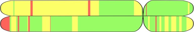
Result of running LAI on chromosome 22 of a Puerto Rican individual from Puerto Rico. Graphics using tagore (Rishishwar et al., 2015). Red, yellow and green represent AFR, EUR and NAT ancestries, respectively
3.2.3 Generalization to unseen species
To further explore the generalization capabilities of our method, we use the parameters learnt with sequences from human individuals (AFR, EUR, SAS and EAS) described in the previous section and evaluate on a dataset composed of DNA sequences from dogs and wolves. The testing dataset contains admixed samples simulated from single-ancestry sequences of Wolf, Terrier and Retriever. Specifically, a total of 29 Wolf, 61 Terrier and 28 Retriever are used to simulate 1270 testing admixed sequences from 2 to 128 generations. Similarly, 12 Wolf, 24 Terrier and 11 Retriever individuals (47 individuals in total) are used as a reference panel to perform inference with SALAI-Net and Loter. Furthermore, we benchmark with LAI-Net, trained with admixed sequences generated from the same 47 founders in the SALAI-Net’s reference panel. Both Loter and LAI-Net are evaluated using their default recommended hyperparameters. Table 2 shows that our model obtains higher accuracy than Loter and LAI-Net when tested on a different species (dogs) than the one it has been trained on (humans). Furthermore, we train a new model with canid genomes as training data and compare it with a model that has been trained with human data. When testing with canid data, the model trained with canids obtains an accuracy of 87.66%, while the model trained with humans an accuracy of 87.26%. This small gap on accuracy highlights the capabilities of the learnt parameters to transfer into completely different inference scenarios.
Table 2.
Accuracy on dog whole-genome data
| Method | Train species | Test species | Accuracy |
|---|---|---|---|
| Loter | – | Dogs | 78.39% |
| LAI-Net | Dogs | Dogs | 86.38% |
| LAI-Net | Humans | Dogs | N/A |
| SALAI-Net | Dogs | Dogs | 87.66% |
| SALAI-Net | Humans | Dogs | 87.27% |
Notes: Human whole genomes included EUR, AFR, SAS and EAS populations.
3.2.4 Computational benchmarking
We compare the memory usage and computational time of SALAI-Net, LAI-Net and Loter when running the models with and without the use of GPU hardware. Since LAI-Net is not ancestry-specific and requires training each time, the time benchmark includes the parameter optimization procedure to fit the model to the specific setting. In Table 3, we present the computation benchmark in the canid dataset. SALAI-Net’s RAM consumption is considerably lower than that of the other systems and it can run without GPU hardware in a reasonable time with almost no additional memory usage. Because some LAI models can be very computationally expensive and require hardware that might not be available, SALAI-Net is a good fit for low-resources settings, even for running on a personal laptop. From a practical perspective, inference can take around 9 h to perform on 300 whole-genome sequences using Loter, while with SALAI-Net more accurate results can be obtained in just minutes. Loter’s Viterbi-like decoding method can be computationally expensive and limits speed. The available Loter implementation allows for CPU multi-core parallelization and we run it on 16 cores. On the other hand, our proposed one-channel one-kernel convolutional smoother layer is extremely computationally light, making the reference matching layer the computational bottleneck in SALAI-Net (due to the computation of window-level cosine similarities). However, we implemented the distances in the reference matching with single matrix multiplication and 2D convolution with stride, taking advantage of Pytorch’s fast implementation and of our available GPU hardware. This large acceleration changes the way users can perform LAI in different species or populations, reducing the time bottleneck.
Table 3.
Comparison of time and memory usage in the dogs dataset
| Method | Hardware | Average sequence time (s) | Time ratio | RAM memory consumption (G) |
|---|---|---|---|---|
| Loter | CPU | 29.83 | × 372 | 15.3 |
| LAI-Net | GPU | 0.279 | × 3.5 | 7.8 |
| LAI-Net | CPU | 2.031 | × 25 | 9.2 |
| SALAI-Net | GPU | 0.080 | × 1 | 2.3 |
| SALAI-Net | CPU | 0.387 | × 4.8 | 2.4 |
Note: Speed ratio is with respect to SALAI-Net on GPU hardware. Results in bold indicate the best performing solution.
4 Discussion
4.1 Relationship with identity by descent
Many genetic applications require interpretable techniques, and, unlike previous machine-learning-based local ancestry approaches, our proposed approach is highly interpretable, as each prediction is obtained by a pattern matching of sequences. This is similar to the identity by descent (IBD) paradigm wherein two segments of a sequence are inferred to be identical by descent (deriving from the same ancestor) if they match closely (Albrechtsen et al., 2009; Browning and Browning, 2010; Gusev et al., 2009; Purcell et al., 2007). SALAI-Net can thus be seen as a smoothed, generalized version of IBD, where ancestry cluster membership is predicted for each window instead of IBD, and the closeness needed for matching and the weighting of different patterns of mismatches is learnt.
4.2 Relationship with kernel and non-parametric methods
The reference matching layer resembles kernel machines and similarity-based methods such as k-nearest neighbour (k-NN) and support vector machines (SVMs). For example, a k-NN classifier provides a classification label through a weighted average of the labels from the k-closest samples given a pre-specified distance metric and a fixed set of weights, whereas our proposed reference matching layer provides a unique score for each ancestry present in the reference panel by performing a weighted sum (with learnt weights) of the top-k cosine similarities. In a similar fashion, SVMs compute a membership score by computing a distance between the input sequence and a set of reference panel (support vectors) with a kernel function and performing a learnt weighted average, where a different weight is assigned to each of the pairwise difference. SVMs differ from our proposed matching layer by how the weighted average is performed: while SVMs require re-training the model once new training samples are present (in order to estimate the weighting coefficient for each sample) our top-k pooling and weighting approach allows reusing the weighting coefficients, since the same coefficients are applied to different samples depending on their ranking within cosine similarity. Therefore, the proposed layer could be understood as a SVM with a cosine similarity kernel, where the linear weights are dynamically assigned conditioned by the cosine similarities.
5 Conclusion
We propose a novel species-agnostic method for LAI based on reference panel matching that outperforms the previous state-of-the-art techniques across multiple different datasets and settings, while enabling an acceleration of up to two orders of magnitude and consuming significantly less memory. When trained with human data, the proposed method shows a very small generalization error gap when applied (without any retraining) to other settings, including other species, demonstrating robust portability across new ancestry groupings, chromosomes, admixture timings and reference panel sizes.
Funding
This paper was published as part of a special issue financially supported by ECCB2022. Some of the computing for this project was performed on the Sherlock cluster at Stanford University. We would like to thank Stanford University and the Stanford Research Computing Center for providing computational resources and support that contributed to these research results. A.G.I. and D.M.M. received support from NIH under award R01HG010140.
Conflict of Interest: AGI is a co-founder of Galatea Bio Inc.
Supplementary Material
Contributor Information
Benet Oriol Sabat, Department of Signal Theory and Communications, Universitat Politecnica de Catalunya, Barcelona 08034, Spain; Department of Biomedical Data Science, Stanford Medical School.
Daniel Mas Montserrat, Department of Biomedical Data Science, Stanford Medical School.
Xavier Giro-i-Nieto, Department of Signal Theory and Communications, Universitat Politecnica de Catalunya, Barcelona 08034, Spain.
Alexander G Ioannidis, Department of Biomedical Data Science, Stanford Medical School; Institute for Computational and Mathematical Engineering, Stanford University, Stanford, CA 94305, USA.
References
- Albrechtsen A. et al. (2009) Relatedness mapping and tracts of relatedness for genome-wide data in the presence of linkage disequilibrium. Genet. Epidemiol., 33, 266–274. [DOI] [PubMed] [Google Scholar]
- Atkinson E.G. et al. (2021) Tractor uses local ancestry to enable the inclusion of admixed individuals in GWAS and to boost power. Nat. Genet., 53, 195–204. [DOI] [PMC free article] [PubMed] [Google Scholar]
- Avallone A. et al. (2020) Local ancestry inference provides insight into tilapia breeding programmes. Sci. Rep., 10, 1–8. [DOI] [PMC free article] [PubMed] [Google Scholar]
- Bergström A. et al. (2020) Insights into human genetic variation and population history from 929 diverse genomes. Science, 367, eaay5012. [DOI] [PMC free article] [PubMed] [Google Scholar]
- Browning S.R., Browning B.L. (2010) High-resolution detection of identity by descent in unrelated individuals. Am. J. Hum. Genet., 86, 526–539. [DOI] [PMC free article] [PubMed] [Google Scholar]
- Consortium I.H. et al. (2010) Integrating common and rare genetic variation in diverse human populations. Nature, 467, 52. [DOI] [PMC free article] [PubMed] [Google Scholar]
- Dias-Alves T. et al. (2018) Loter: a software package to infer local ancestry for a wide range of species. Mol. Biol. Evol., 35, 2318–2326. [DOI] [PMC free article] [PubMed] [Google Scholar]
- Flowers J.M. et al. (2019) Cross-species hybridization and the origin of North African date palms. Proc. Natl. Acad. Sci. USA, 116, 1651–1658. [DOI] [PMC free article] [PubMed] [Google Scholar]
- Gimbernat-Mayol J. et al. (2021) Archetypal analysis for population genetics. bioRxiv. [DOI] [PMC free article] [PubMed]
- Gravel S. (2012) Population genetics models of local ancestry. Genetics, 191, 607–619. [DOI] [PMC free article] [PubMed] [Google Scholar]
- Gusev A. et al. (2009) Whole population, genome-wide mapping of hidden relatedness. Genome Res., 19, 318–326. [DOI] [PMC free article] [PubMed] [Google Scholar]
- Hilmarsson H. et al. (2021) High resolution ancestry deconvolution for next generation genomic data. bioRxiv.
- Ioannidis A.G. et al. (2020) Native American gene flow into Polynesia predating Easter island settlement. Nature, 583, 572–577. [DOI] [PMC free article] [PubMed] [Google Scholar]
- Ioannidis A.G. et al. (2021) Paths and timings of the peopling of Polynesia inferred from genomic networks. Nature, 597, 522–526. [DOI] [PMC free article] [PubMed] [Google Scholar]
- Joukhadar R. et al. (2017) Genetic diversity, population structure and ancestral origin of Australian wheat. Front. Plant Sci., 8, 2115. [DOI] [PMC free article] [PubMed] [Google Scholar]
- Karavani E. et al. (2019) Screening human embryos for polygenic traits has limited utility. Cell, 179, 1424–1435. [DOI] [PMC free article] [PubMed] [Google Scholar]
- Kingma D.P., Ba J. (2014) Adam: A method for stochastic optimization. arXiv preprint arXiv:1412.6980.
- Kong W. et al. (2019) Short-term residential load forecasting based on LSTM recurrent neural network. IEEE Trans. Smart Grid, 10, 841–851. [Google Scholar]
- Kumar A. et al. (2020) Xgmix: Local-ancestry inference with stacked xgboost. bioRxiv.
- Mallick S. et al. (2016) The Simons Genome Diversity Project: 300 genomes from 142 diverse populations. Nature, 538, 201–206. [DOI] [PMC free article] [PubMed] [Google Scholar]
- Mantes A.D. et al. (2022) Neural admixture: rapid population clustering with autoencoders. bioRxiv.
- Maples B.K. et al. (2013) Rfmix: a discriminative modeling approach for rapid and robust local-ancestry inference. Am. J. Hum. Genet., 93, 278–288. [DOI] [PMC free article] [PubMed] [Google Scholar]
- Marnetto D. et al. (2020) Ancestry deconvolution and partial polygenic score can improve susceptibility predictions in recently admixed individuals. Nat. Commun., 11, 1–9. [DOI] [PMC free article] [PubMed] [Google Scholar]
- Martin A.R. et al. (2017) Human demographic history impacts genetic risk prediction across diverse populations. Am. J. Hum. Genet., 100, 635–649. [DOI] [PMC free article] [PubMed] [Google Scholar]
- Montserrat D.M. et al. (2019) Class-conditional vae-gan for local-ancestry simulation. arXiv preprint arXiv:1911.13220.
- Montserrat D.M. et al. (2020) Lai-net: local-ancestry inference with neural networks. In: ICASSP 2020–2020 IEEE International Conference on Acoustics, Speech and Signal Processing (ICASSP). IEEE, pp. 1314–1318. [Google Scholar]
- Oord A. v d. et al. (2016) Wavenet: a generative model for raw audio. arXiv preprint arXiv:1609.03499.
- Padhukasahasram B. (2014) Inferring ancestry from population genomic data and its applications. Front. Genet., 5, 204. [DOI] [PMC free article] [PubMed] [Google Scholar]
- Paszke A. et al. (2019) Pytorch: An imperative style, high-performance deep learning library. In: Wallach,H. et al. (eds.) Advances in neural information processing systems. Vol. 32, Curran Associates, Inc., pp. 8024–8035.
- Perera M. et al. (2022) Generative moment matching networks for genotype simulation. bioRxiv. [DOI] [PubMed]
- Plassais J. et al. (2019) Whole genome sequencing of canids reveals genomic regions under selection and variants influencing morphology. Nat. Commun., 10, 1–14. [DOI] [PMC free article] [PubMed] [Google Scholar]
- Price A.L. et al. (2009) Sensitive detection of chromosomal segments of distinct ancestry in admixed populations. PLoS Genet., 5, e1000519. [DOI] [PMC free article] [PubMed] [Google Scholar]
- Purcell S. et al. (2007) Plink: a tool set for whole-genome association and population-based linkage analyses. Am. J. Hum. Genet., 81, 559–575. [DOI] [PMC free article] [PubMed] [Google Scholar]
- Raghavan M. et al. (2015) Genomic evidence for the pleistocene and recent population history of native Americans. Science, 349, aab3884. [DOI] [PMC free article] [PubMed] [Google Scholar]
- Ren Y. et al. (2019) Fastspeech: fast, robust and controllable text to speech. arXiv preprint arXiv:1905.09263.
- Rishishwar L. et al. (2015) Ancestry, admixture and fitness in Colombian genomes. Sci. Rep., 5, 12376–12316. [DOI] [PMC free article] [PubMed] [Google Scholar]
- Sankararaman S. et al. (2008) Estimating local ancestry in admixed populations. Am. J. Hum. Genet., 82, 290–303. [DOI] [PMC free article] [PubMed] [Google Scholar]
- Siva N. (2008) 1000 Genomes project. Nat. Biotechnol., 26, 256–257. [DOI] [PubMed] [Google Scholar]
- Suarez-Pajes E. et al. (2021) Genetic ancestry inference and its application for the genetic mapping of human diseases. Int. J. Mol. Sci., 22, 6962. [DOI] [PMC free article] [PubMed] [Google Scholar]
- Sundquist A. et al. (2008) Effect of genetic divergence in identifying ancestral origin using HAPAA. Genome Res., 18, 676–682. [DOI] [PMC free article] [PubMed] [Google Scholar]
- Tang H. et al. (2006) Reconstructing genetic ancestry blocks in admixed individuals. Am. J. Hum. Genet., 79, 1–12. [DOI] [PMC free article] [PubMed] [Google Scholar]
- Thornton T.A., Bermejo J.L. (2014) Local and global ancestry inference and applications to genetic association analysis for admixed populations. Genet. Epidemiol., 38, S5–S12. [DOI] [PMC free article] [PubMed] [Google Scholar]
- Vaswani A. et al. (2017) Attention is all you need. In: Guyon,I. et al. (eds.) Advances in Neural Information Processing Systems, Vol. 30, Curran Associates, Inc., pp. 5998–6008.
- Voulodimos A. et al. (2018) Deep learning for computer vision: a brief review. Comput. Intell. Neurosci., 2018, 7068349. [DOI] [PMC free article] [PubMed] [Google Scholar]
- Zaheer M. et al. (2020) Big bird: Transformers for longer sequences. In: Larochelle,H. et al. (eds.) Advances in Neural Information Processing Systems, Vol. 33, Curran Associates, Inc., pp. 17283–17297.
Associated Data
This section collects any data citations, data availability statements, or supplementary materials included in this article.