Singular value decomposition of protein sequences as a method to visualize sequence and residue space

Abstract

Singular value decomposition (SVD) of multiple sequence alignments (MSAs) is an important and rigorous method to identify subgroups of sequences within the MSA, and to extract consensus and covariance sequence features that define the alignment and distinguish the subgroups. This information can be correlated to structure, function, stability, and taxonomy. However, the mathematics of SVD is unfamiliar to many in the field of protein science. Here, we attempt to present an intuitive yet comprehensive description of SVD analysis of MSAs. We begin by describing the underlying mathematics of SVD in a way that is both rigorous and accessible. Next, we use SVD to analyze sequences generated with a simplified model in which the extent of sequence conservation and covariance between different positions is controlled, to show how conservation and covariance produce features in the decomposed coordinate system. We then use SVD to analyze alignments of two protein families, the homeodomain and the Ras superfamilies. Both families show clear evidence of sequence clustering when projected into singular value space. We use k‐means clustering to group MSA sequences into specific clusters, show how the residues that distinguish these clusters can be identified, and show how these clusters can be related to taxonomy and function. We end by providing a description a set of Python scripts that can be used for SVD analysis of MSAs, displaying results, and identifying and analyzing sequence clusters. These scripts are freely available on GitHub.

1. INTRODUCTION

The multiple sequence alignment (MSA) is an essential tool for representing the sequence features that define a protein family, highlighting both similarities and differences among family members. These features contain information on structure, function, stability, and taxonomy. There are several approaches to extract such information from sequence alignments, including construction of phylogenetic trees, determination of consensus sequences, and analysis of covariance among residues at different positions using techniques such as direct coupling analysis ¹ , ² , ³ and sector analysis. ⁴ , ⁵

Another technique to extract information on consensus, covariance, and taxonomy from MSAs is singular value decomposition (SVD). SVD and its close relative, principal component analysis (PCA), are mathematically rigorous dimensionality reduction techniques that are often presented in linear algebra courses (see Appendix S1 for a comparison of SVD and PCA). These techniques have become popular tools in the machine‐learning toolbox, and have been used in diverse areas such as climate research ⁶ and population genetics. ⁷ , ⁸ , ⁹ , ¹⁰

In a pioneering study a quarter century ago, Caseri et al. used SVD to analyze protein sequence alignments. ¹¹ In the intervening period, SVD has been used to guide studies of specificity and stability in protein sequences in a handful of studies, ⁵ , ¹² and has been used to group aligned proteins based on substitution matrix scoring. ¹³ However, the mathematical basis of dimensionality reduction techniques such as SVD and PCA remain unfamiliar to many protein scientists. As a result, the application of this powerful technique to protein sequence analysis has been underutilized.

Singular value decomposition of an MSA transforms the sequences into a new coordinate system. This coordinate system, which involves eigenvectors associated with the MSA matrix, provides a much simpler representation than the original sequence alignment. Although all of the information from the MSA is preserved by SVD, it is concentrated along a relatively small number of coordinate axes. Importantly, the coordinates of sequences in SVD space are uncorrelated from one another, unlike the original MSA. This new space can be used to depict sequences, providing a quantitative view of sequence space. Inspection of the sequences within this space often reveals clusters that may reflect sequence phylogeny and/or functional specialization. In addition, SVD can be used to identify the individual residues that define phylogeny and specialization.

In this review, we describe the mathematics of SVD as it applies to MSAs. Our goal is to be simple enough to be intuitive, but rigorous enough to be implemented by readers. After introducing the equations of SVD, we analyze toy models to show how sequence conservation and residue covariance project into singular coordinate space. Next, we apply full SVD analysis to alignments of homeodomain and Ras family GTPases, and show how clustering in SVD space can be used to identify sequence subfamilies within the MSA. We then present a method for identifying the residues that define different subfamilies. Next, we examine how sequence clusters in SVD space relate to taxonomy, and show how functional information can be mapped to sequence clusters. We end with a brief description of a suite of Python scripts for these analyses that is available on GitHub.

2. THE MATHEMATICS OF SINGULAR VALUE DECOMPOSITION AND EIGENDECOMPOSITION

SVD is a mathematical technique that is applied to matrices of numerical values. Although a MSA has the form of a matrix (with m rows and $\ell$ columns, where m is the number of sequences in the alignment and $\ell$ is the number of residues in each aligned sequence plus the number of gaps to the alignment; Figure 1a), its elements are letters corresponding to the 20 amino acids and a gap character. To apply SVD to an MSA, these 21 letters must be converted to numerical values that are distinct but carry equal weight, to avoid making some residues more important than others.

FIGURE 1.

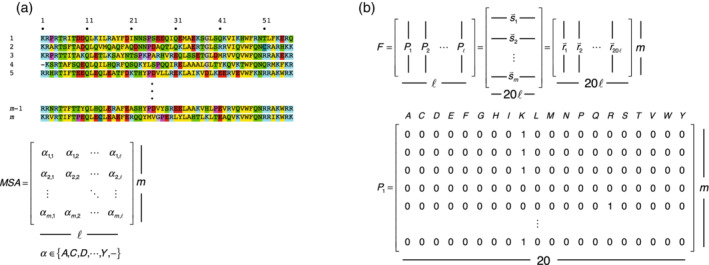
Matrix representation of a multiple sequence alignment. (a) A multiple sequence alignment (top) of $m$ sequences of length $\ell$= 56 residues. The alignment can be thought of as a matrix of $m$ rows and $\ell$ columns, where each matrix element is one of the 20 amino acids ($\alpha$) along with the gap residue. (b) A binary representation F of the MSA matrix, where each position is represented by an $m$ by $20$ block matrix $P$. Each column of the block matrix corresponds to one of the 20 amino acids at a given position. Each row in the block matrix corresponds to a position in a particular sequence in the MSA, and contains a one in the column corresponding to the amino acid at that position and zeros in all other columns. If a sequence $i$ contains a gap at a particular position, row $i$ of the corresponding block matrix contains 20 zeros. F can be viewed as (i) a collection of m binary sequence row vectors ${\stackrel{\rightharpoonup }{s}}_i$, each of length $20\ell$ or (ii) a collection of $20\ell$ binary residue column vectors ${\stackrel{\rightharpoonup }{r}}_i$, each of length $m.$

To assign residues numerical values of equal importance, each of the $\ell$ MSA positions is expanded to 20 separate variables corresponding to each of the 20 residues. Each variable takes a value of one if the residue occurs in a particular sequence, and zero otherwise (Figure 1). This binary or “one‐hot” encoding scheme increases the number of residue variables from $\ell$ to $20\ell$. In principle, gaps could be included as a 21st variable, although doing so introduces no new information, since the presence of a gap is implied when each of the 20 non‐gap residue variables has a value of 0. Figure 1b shows this binary representation using $m$ by $20$ block matrices for each position ($P_i$ at position $i$).

2.1. Singular value decomposition of the F‐matrix

SVD factors the F matrix into a product of three matrices according to the formula

$$F=U\mathrm{\sum }{V}^T,$$ (1)

$U$ is an $m$ by $m$ matrix of normalized^* column vectors ${\stackrel{\rightharpoonup }{u}}^{\left(i\right)}$, which we will refer to as “sequence eigenvectors”^† (Figure 2). $V^T$ is a $20\ell$ by $20\ell$ matrix of normalized row vectors ${\stackrel{\rightharpoonup }{v}}^{(i)}$ (the columns of matrix V), referred to as “residue eigenvectors.” vectors ${\stackrel{\rightharpoonup }{v}}^{(i)}$ (the columns of matrix $V$), referred to as “residue eigenvectors.” One important feature of the decomposition is that $U$ and $V^T$ are orthogonal matrices; thus, ${\stackrel{\rightharpoonup }{u}}^{(i)}$ and ${\stackrel{\rightharpoonup }{v}}^{(i)}$ are orthogonal. $\sum$ is an $m$ by $20\ell$ rectangular diagonal matrix with numbers ${\sigma }_i$, referred to as “singular values,” along the main diagonal, and zeros elsewhere (Figure 2). Note that there will be at most $\min \left(m, 20\ell \right)$ singular values.^‡

FIGURE 2.

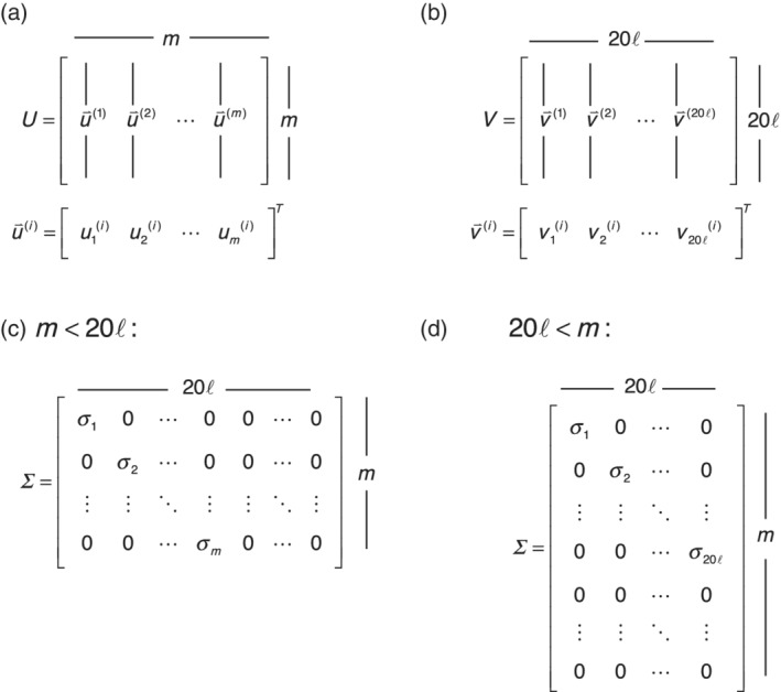
Features of the matrices in singular value decomposition. (a,b) Sequence and residue eigenvector matrices U and V , along with the i ^th singular vector for each matrix. (c, d) Singular value matrices. In (c), the number of rows (sequences) is small compared to the binary encoding of the sequence length (20 times residues plus gap positions in the MSA). In (d), the number of rows (sequences) is large compared to the binary sequence length.

It is customary to scale the vectors ${\stackrel{\rightharpoonup }{u}}^{(i)}$ and ${\stackrel{\rightharpoonup }{v}}^{(i)}$ so that they are of unit length, and to scale the ${\sigma }_i$ values so that Equation (1) is preserved. It is also customary to arrange the entries in $\sum$ in decreasing order along the diagonal, and to rearrange the columns of $U$ and rows of $V^T$ accordingly. The largest ${\sigma }_i$ value is referred to as the first singular value, the next largest as the second singular value, and so on. The associated singular vectors are similarly named.

2.2. Finding the singular value decomposition through eigendecomposition

Section 2.1 gives the form of SVD, but does not describe how this decomposition is found. One way to find $U$, $V$, and $\mathrm{\sum }$ is to multiply $F$ and its transpose to form the product $C=F{F}^T$ and $D=F^{T}F$ and then find the eigenvectors and eigenvalues of these two products. As is demonstrated in Appendix S1, these eigenvectors are equal to the columns of $U$ and $V$ (and thus the rows of $V^T$), and the eigenvalues are equal to the squares of the singular values in $\mathrm{\sum }$.

In addition to providing a route to calculating the SVD of matrix $F$, the $C$ and $D$ matrices provide complementary views of the sequences and residues of the MSA. The elements of the $C$ matrix count the number of identities between pairs of sequences, and the elements of the $D$ matrix count the number of pairs of residues of a particular type at two positions. The $C$ and $D$ matrices are also the starting point for PCA.

3. VISUALIZING SEQUENCES AND RESIDUES IN SINGULAR VALUE DECOMPOSITION SPACE

An advantage of concentrating the information in an MSA into a handful of SVD coordinates is that sequences and residues can be directly visualized in a low‐dimensional space. This contrasts with the starting MSA and F matrices, which are distributed over too many dimensions to be visualized. In this section, we will describe how to project MSA sequences into SVD space, how to project homologous sequences not in the MSA into SVD space, and how to project specific residues into SVD space.

3.1. Visualizing sequences from the multiple sequence alignment in singular value decomposition space

For a given sequence $i$ from the MSA, the numerical value associated with the k ^th singular coordinate is proportional to the corresponding element in the sequence eigenvector, that is, $u^{\left(k\right)}$. In other words, the ${\stackrel{\rightharpoonup }{u}}^{(k)}$ vectors give the coordinates of each MSA sequence in the k ^th singular dimension. Thus, plotting the elements of the first few sequence eigenvectors provides a quantitative view of sequence space.

The algebra that demonstrates this approach is given in Appendix S2. The key result from this derivation the following identity:

$${\stackrel{\rightharpoonup }{s}}_i·{\stackrel{\rightharpoonup }{v}}^{\left(k\right)}={\sigma }_k{u}_i^{\left(k\right)}$$ (2)

Since the sequence vectors $\stackrel{\rightharpoonup }{s_i}$ are binary vectors with ones marking each residue, the dot product on the left side of Equation (2) sums the elements of the residue eigenvector ${\stackrel{\rightharpoonup }{v}}^{(k)}$ corresponding to the residues in sequence $i$. Since ${\stackrel{\rightharpoonup }{v}}^{(k)}$ is normalized, this dot product can be viewed as the projection of the sequence vector $\stackrel{\rightharpoonup }{s_i}$ onto the residue eigenvector ${\stackrel{\rightharpoonup }{v}}^{(k)}$. Equation (2) says that rather than taking this dot product for each sequence, the projection can be directly read off as the i ^th element of the k ^th sequence eigenvector ${\stackrel{\rightharpoonup }{u_i}}^{(k)}$ scaled by the corresponding singular value ${\sigma }_k$. Thus, the sequences in the MSA can be plotted in the first d dimensions of SVD space simply by plotting the elements of ${\sigma }_1{\stackrel{\rightharpoonup }{u}}^{(1)}$ through ${\sigma }_d{\stackrel{\rightharpoonup }{u}}^{(d)}$.

3.2. Visualizing sequences not in the multiple sequence alignment in singular value decomposition space

Sequences not in the MSA can also be projected into SVD space, but they must first be aligned with the MSA. Once aligned, the new sequence can be converted to binary form and dotted with the residue eigenvectors of interest in the same way that MSA sequences are projected:

$$\stackrel{\rightharpoonup }{t}·{\stackrel{\rightharpoonup }{v}}^{(k)}={\sigma }_k{\tau }^{\left(k\right)}$$ (3)

where $\stackrel{\rightharpoonup }{t}$ is an aligned binary‐encoded sequence and ${\tau }^{\left(k\right)}$ is the value of sequence $\stackrel{\rightharpoonup }{t}$ along the k ^th coordinate. Such projections are useful for identifying which cluster a new extant sequence belongs to, or for examining designed sequences such as consensus or ancestral sequences.

3.3. Visualizing residues from the multiple sequence alignment into singular value decomposition space

Residue coordinates in SVD space are derived from the elements of residue eigenvectors ${\stackrel{\rightharpoonup }{v}}^{(k)}$. Justification parallels the derivation in the previous section that connected ${\stackrel{\rightharpoonup }{u_i}}^{(k)}$ to MSA sequences (Appendix S2). Briefly, transposing Equation (1) and right‐multiplying by U gives

$$F^{T}U=V{\mathrm{\sum }}^T$$ (4)

Expansion of the matrix products in Equation (4) (Figure S3B) leads to a set of $20\ell$ equations of the form

$$\stackrel{\rightharpoonup }{r_i}\bullet {\stackrel{\rightharpoonup }{u}}^{(k)}={\sigma }_k{v}_i^{\left(k\right)}$$ (5)

analogous to Equation (2). Due to the binary encoding of the $\stackrel{\rightharpoonup }{r_i}$ residue vectors, the dot product on the left side of Equation (5) sums the subset of elements from ${\stackrel{\rightharpoonup }{u}}^{(k)}$ for which the corresponding sequences contain the residue represented by $v_i^{\left(k\right)}$. Equation (5) says that this dot product can be read off as the i ^th element of the k ^th residue eigenvector, $v_i^{\left(k\right)}$. Plotting the $20\ell$ elements $v_i^{\left(k\right)}$ in the first $d$ dimensions of SVD space gives a residue‐based picture of sequence space that complements that obtained from plotting sequence coordinates ${\sigma }_k{u}_i^{\left(k\right)}$.^§

4. SIMPLIFIED EXAMPLES OF SEQUENCE BIAS AND SEQUENCE COVARIANCE

In this section, we apply SVD to simple sequence models that contain different amounts of sequence conservation and covariance to explore how conservation and covariance influence sequence and residue coordinates in SVD space. In these models, we include just three positions (analogous to a three‐residue protein). At each position, there are just two types of residues: A and B at position 1, C and D at position 2, and E and F at position 3.

4.1. How sequence features determine residue coordinates in singular value decomposition space

In the first set of models (models I.ef and I.bf, Figure 3), residues at different positions are independent of one another. That is, the probabilities of having a pair of residues at two positions is the product of the marginal probabilities of the two residues. In model I.ef (Figure 3, top), all six residues have equal frequencies, corresponding to residue probabilities of 0.5, pair probabilities of 0.25, and three‐residue sequence probabilities of 0.125. This leads to a relatively flat residue count matrix $D$, reflecting uniform pair counts for residues at different positions. However, there are high (but equal) counts along the main diagonal, and zeros adjacent to the diagonal which reflect anticorrelation between residues at the same position.

FIGURE 3.

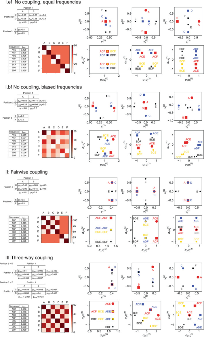
The effects of bias and coupling on SVD coordinates of residues and sequences. A simple three‐position sequence with two residues at each position (A, B at position 1, C, D at position 2, and E, F at position 3) is used to generate MSAs with varying degrees of sequence bias and coupling. In model I.ef (top), the six residues have equal overall frequencies (of 0.5). In model I.bf (upper middle), the six residues occur with different frequencies, as given by the marginal probabilities (e.g., p _A) in the table on the lower left. In both versions of model I, residue frequencies are independent of each other, such that residue pair probabilities are given by the product of the marginal probabilities. In model II (lower middle), there is pairwise covariance between positions 1 and 2, but position 3 is independent of the other two. In model III (bottom), there is three‐way covariance between positions 1, 2, and 3. For each model, joint and marginal probabilities and probabilities for the eight different sequences are given in the upper left, residue pair count matrices ($D=F^{T}F$) are shown in the lower left, residue $v_i^{\left(k\right)}$ values along singular coordinates 1–4 are shown in the upper right, and sequence ${\sigma }_k{u}_i^{\left(k\right)}$ values along singular coordinates 1–4 are shown in the lower right.

Given that model I.ef has the largest entropy,^¶ the SVD would be expected to be rather featureless. Indeed, residue positions $v_i^{\left(k\right)}$ along the first singular coordinate are all the same for each of the six residues (Figure 3, top right). However, there is considerable variation in coordinates 2, 3, and 4, where pairs of residues have opposite values. These variations result from anticorrelated residue pairs at the same position (e.g., residues E and F at position 3, which have opposite $v_i^{\left(2\right)}$, Figure 3, top right).

In contrast to the equal‐frequency model, the biased frequency model (I.bf) shows considerable variation of residue $v_i^{\left(1\right)}$ values along the first singular coordinate (Figure 3, upper middle). These values correlate with the frequency of each residue: A has the highest frequency and has the largest $v^{\left(1\right)}$ value, whereas B has the lowest frequency and the smallest $v^{\left(1\right)}$ value. Indeed, a plot of $v_i^{\left(1\right)}$ values for model I.bf shows a roughly linear correlation between $v_i^{\left(1\right)}$ and residue frequency (Figure 4a).

FIGURE 4.

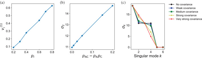
The effects of sequence bias and correlation on residue coordinates and singular values. (a) For model I.bf, where residues at the same position have different probabilities (Figure 3), the residue $v_i^{\left(1\right)}$ values along the first singular coordinate are correlated with the residue probability. (b) for model II, where there is a pairwise correlation between residues A and C at positions 1 and 2, the singular value ${\sigma }_2$ is correlated with covariance between residues A and C (likewise for residues B and D, not shown). (c) For model II, as the strength of the pairwise covariance increases, ${\sigma }_2$ increases at the expense of ${\sigma }_4$, indicating that when correlation increases, fewer components are needed in the SVD.

As with the equal frequency model, there is also variation in residue $v_i^{\left(k\right)}$ values along higher singular coordinates ($k\ge 2$; Figure 3, bottom right). Again, this variation results from pairs of residues at the same position having opposite $v_i^{\left(k\right)}$ values, reflecting anticorrelation. Another general feature of residue SVD plots (i.e., $v_i^{\left(k\right)}$ versus $v_i^{\left(j\ne k\right)}$) is that there is no correlation between values; this also holds for sequence plots (i.e., $u_i^{\left(k\right)}$ vs. $u_i^{\left(j\ne k\right)}$). A linear fit to the points in any of the three right‐most plots in Figure 3 would return a correlation coefficient of zero since the SVD produces orthogonal ${\stackrel{\rightharpoonup }{v}}^{(k)}$ (and ${\stackrel{\rightharpoonup }{u}}^{(k)}$) vectors, that is, ${\stackrel{\rightharpoonup }{v}}^{(k)}·{\stackrel{\rightharpoonup }{v}}^{(j)}=0$ (and ${\stackrel{\rightharpoonup }{u}}^{(k)}·{\stackrel{\rightharpoonup }{u}}^{(j)}=0$) for $k\ne j$.^**

To examine the effects of covariance between residues at different position, we modified model I.ef (with equal residue frequencies at each position) to include covariance between residues at positions 1 and 2 (model II, Figure 3). Specifically, the frequency of sequences with both A at position 1 and C at position 2 was increased, relative to what would be expected from marginal probabilities (and likewise with B and D). Because residues all have equal probabilties in this model, there is no dispersion of $v_i^{\left(1\right)}$ values (Figure 3), again reflecting the fact that the first singular coordinate is a measure of conservation. However, unlike the uncorrelated equal frequency model (I.ef), there is mutual displacement of positively correlated residues in the second singular coordinate: $v_i^{\left(2\right)}$ values for residues A and C are displaced in the positive direction, whereas values for residues B and D are displaced in the negative direction, opposite to A and C. Thus, the coupling between residues at different positions in model II is revealed in singular coordinate two. This is unlike model I, where variation in the second singular coordinate reflects anticorrelation of residues at the same position. The anticorrelation of residues at the same position is instead pushed to the third and fourth singular coordinates. Residues at position 3 (E and F) are oppositely shifted in the third singular coordinate, and residues at positions 1 (A and B) and 2 (C and D) are oppositely shifted in the fourth singular coordinate.

Perhaps counterintuitively, although displacement of $v_i^{\left(2\right)}$ values result from pairwise covariance, the extent of displacement does not depend on the strength of the covariance (not shown; this is also true for $v_i^{\left(j>2\right)}$ values). Instead, the increased coupling in model II increases the corresponding singular value ${\sigma }_2$ (Figure 4b). This increase in ${\sigma }_2$ (with increased coupling is compensated by a decrease in ${\sigma }_4$).

To further investigate how sequence covariance influences the position of residue $v_i^{\left(k\right)}$ values in SVD space, we built a third model where residues at all three positions are positively coupled (model III, Figure 3). This three‐way correlation may be considered to be mimic the higher‐order covariances generated in MSAs containing multiple phylogenetically distinct subfamilies. In model III, the ${v_i}^{\left(2\right)}$ values for all three positively coupled residues (e.g., A, C, and E) are displaced in the same direction, opposite the other three residues (e.g., B, D, and F). It is noteworthy that this three‐residue coupling is captured in a single SVD coordinate. Again, anticorrelation between residues at the same position is revealed in singular coordinates 3 and 4 (Figure 3, bottom right).

Summarizing the findings from the toy models, uncorrelated residue biases result in displacements in singular coordinate one. Positive covariance between residues at different positions results in the mutual displacements of positively covarying residues (e.g., A and C in model II) in the second singular coordinate, and opposite displacements from the negatively covarying residues (e.g., A and D in model II). Opposite displacements are also seen for anticorrelated residues at the same position.

4.2. How residue coordinates determine sequence coordinates in singular value decomposition space

As described above, the coordinates ${\sigma }_k{u}_i^{\left(k\right)}$ of each MSA sequence in SVD space can be obtained from the corresponding elements of the sequence eigenvectors ${\stackrel{\rightharpoonup }{u}}^{(k)}$. Here, we will use our toy model to illustrate how these sequence coordinates are obtained from residue coordinates $v_i^{\left(k\right)}$. This connection is made through Equation (2), which can be written as a summation:

$${\sigma }_k{u}_i^{\left(k\right)}=\stackrel{\rightharpoonup }{s_i}\cdot {\stackrel{\rightharpoonup }{v}}^{(k)}=\sum _{j\in \stackrel{\rightharpoonup }{s_i}}{v}_j^{\left(k\right)}$$ (6)

Because of the binary nature of $\stackrel{\rightharpoonup }{s_i}$, the dot product between $\stackrel{\rightharpoonup }{s_i}$ and $v_j^{\left(k\right)}$ selects only the $v_j^{\left(k\right)}$ values that correspond to the $\ell$ residues in sequence $i$. Thus, Equation (6) provides a simple recipe to get the coordinate of $i$ in the k ^th singular dimension: take the $v_i^{\left(k\right)}$ values corresponding to residues in the sequence and sum them. This is demonstrated for a six‐residue sequence model in SVD coordinates 1 and 2 (Figure 5) using a vector sum. For the three‐residue sequence ACE, the coordinates of each of the three residues A, C, and E can be represented as arrows starting at the origin and end at the corresponding residue coordinate pair ($v_i^{\left(1\right)}$, $v_i^{\left(2\right)}$) (dashed arrows). When these vectors are arranged head to tail (giving the vector sum, solid arrows), the result ends at the coordinate for sequence ACF.

FIGURE 5.

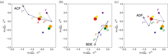
The coordinates each sequence in SVD space is the sum of the coordinates of its residues. Singular value decomposition of a three‐position, six‐residue model described above was used to generate sequence coordinates ${\sigma }_k{u}_i^{\left(k\right)}$ and residue coordinates $v_j^{\left(k\right)}$. In this model, there is sequence bias at each position (p _A = 0.8, p _B = 0.2, p _C = 0.7, p _D = 0.3, p _E = 0.6, p _F = 0.4) as well as pairwise correlation between positions 1 and 2 (p _AC = 0.65, p _AD = 0.15, p _BC = 0.05, p _BD = 0.15). Each of the six residues are plotted in the first and second singular dimensions ($v_i^{\left(1\right)}$, $v_i^{\left(2\right)}$; circles and dashed arrows) along with one sequence (${\sigma }_1{u}_i^{\left(1\right)}$, ${\sigma }_2{u}_i^{\left(2\right)}$; plus sign) per panel. SVD, singular value decomposition

This summation can be used to rationalize the distribution of sequences from the toy models above. For example, in the SVD plane depicting the first and second singular coordinates for model 1.bf (sequence bias without coupling), sequences are separated into two clusters along the second coordinate by the identity at position 3 (E vs. F), because this is the coordinate that separates $v_E^{\left(2\right)}$ and $v_F^{\left(2\right)}$. Within these two clusters, sequences are arranged along the first coordinate by the marginal probabilities of residues at positions 1 and 2: sequences with A are furthest to the right, whereas those with B are furthest to the left. For model II (pairwise coupling), sequences are clustered along the second coordinate depending on whether they have the correlated AC residue pair (which both have positive $v_i^{\left(2\right)}$ values) or the correlated BD residue pair (with negative $v_i^{\left(2\right)}$ values). Although there are also sequences between these clusters, they contain an anticorrelated pair at positions 1 and 2 (AD or BC), and thus occur infrequently in the MSA. Thus, when the entire MSA is plotted in SVD space, the density of sequences will be enriched at the AC and BD clusters and depleted at the AD and BC locus.

5. SINGULAR VALUE DECOMPOSITION OF HOMEODOMAIN AND RAS FAMILY SEQUENCES

In this and the remaining sections, we will present SVD of MSAs from two protein families. The first of these is the homeodomain (HD) family. Homeodomains are small (~57 residue) DNA‐binding domains found in eukaryotes. ¹⁴ , ¹⁵ , ¹⁶ We present results for HD in part because much work has been done to characterize the specificity and stability of HDs, ¹⁷ , ¹⁸ , ¹⁹ , ²⁰ , ²¹ and HDs have been the subject of consensus‐based protein design using MSA information. ²² , ²³ , ²⁴ The second family is the Ras superfamily, which includes the well‐characterized Ras, Rab, Rho, Ran, and Arf subfamilies ²⁵ in eukaryotes, along with less‐well characterized homologues in bacteria. ²⁶ Ras domains are small (~160 residue) GTPases involved in signaling pathways for cell growth and apoptosis. In addition to illustrating how SVD can be used to identify and group subfamilies of sequences, we include the Ras family to compare with the pioneering analysis of Casseri et al. ¹¹ which presented an SVD of Ras, albeit with many fewer sequences than are available today.

Since MSAs are the starting point for SVD analysis, the details of selecting and aligning sequences are important. Here, we follow a protocol previously used for consensus design. ²⁷ Briefly, we collect a large number of sequence homologues, either in a pre‐aligned form (from Pfam, e.g., ²⁸ ) or by searching sequence databases. Sequences with >90% identity are removed, and sequences that are shorter or longer than the median sequence length by 30% are removed. This length‐filtered set is re‐aligned, and positions where gap residues occur in more than 50% of the sequences are eliminated.

Using the procedures described above, we have generated MSAs for HD (PF00046) and Ras (PF00071). Initial HD and Ras alignments containing 85,650 and 45,751 sequences were downloaded from Pfam (version 34.0) and curated as described above to give 4,995 and 10,265 sequences in the final alignments, respectively. One‐hot encoding and SVD was performed on these two alignments using in‐house Python scripts (described below).

For each family, the first 20 singular values are shown in Figure 6. In both cases, the first singular value is significantly larger than the others ($\left({\sigma }_1|{\sigma }_2\right)\approx 3.3\text{and}3.1$ for HD and Ras, respectively), reflecting the high signal associated with single‐residue conservation. Subsequent singular values decrease more gradually (Figure 6). Although singular values remain relatively high past ${\sigma }_{20}$, much of this results from the trivial anticorrelation of different residues at the same position, as is demonstrated by randomly shuffling each column in either the MSA or F‐matrix (Figure 6, red and blue bars, respectively).

FIGURE 6.

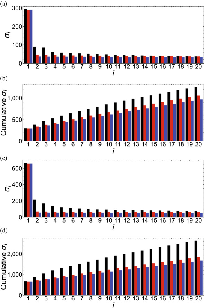
Singular values for homeodomain and Ras. (a,c) Singular values and (b,d) cumulative singular values for homeodomain (a,b) and Ras (c,d) are shown in black bars. Red bars are singular values for an MSA where residues in each column is randomly shuffled, eliminating sequence covariance. Blue bars are singular values for an 𝐹‐matrix where each column is randomly shuffled. In total, the singular values sum to 9,646 and 37,273 for HD and Ras, respectively. MSA, multiple sequence alignment

To visualize the sequence space of HD and Ras in the SVD coordinate system, we generated 2D plots of adjacent ${\sigma }_k{u}_i^{\left(k\right)}$, ${\sigma }_{k+1}{u}_i^{\left(k+1\right)}$ pairs from $k=1$ to $k=4$, and 3D plots of ${\sigma }_1{u}_i^{\left(1\right)}$, ${\sigma }_2{u}_i^{\left(2\right)}$, and ${\sigma }_3{u}_i^{\left(3\right)}$ triples (Figure 7). One striking feature of these sequence scatter plots is that all sequences are displaced in the same direction along the first singular coordinate, whereas for $k\ge 2$ the ${\sigma }_k{u}_i^{\left(k\right)}$ values are centered on zero. Displacement of ${\sigma }_1{u}_i^{\left(1\right)}$ values results from the relationship between conservation and the first singular coordinate; since shared sequence similarity is a requirement for inclusion in the MSA, all sequences are displaced in the same direction. The correlation between conservation and ${\sigma }_1{u}_i^{\left(1\right)}$ values can be seen by plotting ${\sigma }_1{u}_i^{\left(1\right)}$ versus the number of identities each MSA sequence has with the overall consensus sequence (Figure S4); both HD and Ras show a roughly linear correlation, with Pearson correlation coefficients of 0.942 and 0.973. The relationship between conservation and the first singular coordinate is further highlighted by projecting the consensus sequences calculated from each MSA into SVD space using Equation (3) (pink stars, Figure 7). These consensus sequences are farther from zero along the first singular coordinate than any of the MSA sequences because consensus sequences capture conservation to a greater extent than any of the MSA sequences.

FIGURE 7.

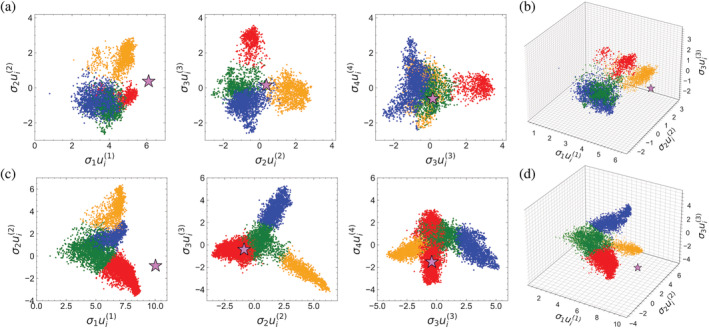
The sequence spaces of HD and Ras generated by SVD. Each point corresponds to a single HD (a,b) or Ras superfamily sequence (c,d) from the MSAs analyzed by SVD. Pink stars are consensus sequences derived from the entire MSA. k‐Means clustering was performed on ${\sigma }_1{u}_i^{\left(1\right)}$, ${\sigma }_2{u}_i^{\left(2\right)}$, and ${\sigma }_3{u}_i^{\left(3\right)}$ values to assign sequences to one of four clusters (colored red, blue, orange, and green). To visualize the 3D plots from different angles, see Videos S1 and S2. MSA, multiple sequence alignment; SVD, singular value decomposition

In addition to conservation, differences in the lengths of the curated sequences in the MSA gives rise to variation in ${\sigma }_1{u}_i^{\left(1\right)}$ values. Though all sequences are aligned to an MSA of length $\ell$, they have different lengths owing to different numbers of gap characters.^†† As illustrated in Figure 5, the ${\sigma }_1{u}_i^{\left(1\right)}$ value for sequence $i$ is equal to the sum of the elements in ${\stackrel{\rightharpoonup }{v}}^{(1)}$ that correspond to non‐gap residues in that sequence (Equation 6). Long sequences sum up more ${\stackrel{\rightharpoonup }{v}}^{(1)}$ terms than short sequences, elements of ${\stackrel{\rightharpoonup }{v}}^{(1)}$ all have the same sign, the sum (which is equal to ${\sigma }_1{u}_i^{\left(1\right)}$) is larger. This is illustrated in Figure S5, which shows a correlation between sequence lengths (excluding gap characters) and ${\sigma }_1{u}_i^{\left(1\right)}$ values. It is worth noting that the correlation between ${\sigma }_1{u}_i^{\left(1\right)}$ and length is not as strong as that with consensus identities (compare Figures S4 and S5).

A key feature of the ${\sigma }_k{u}_i^{\left(k\right)}$ plots for HD and Ras is that the sequences are not distributed uniformly in SVD space, but are partitioned into discrete clusters and projections. These features are most pronounced for the first few singular coordinates, although they persist beyond ${\sigma }_4{u}_i^{\left(4\right)}$ (Figures S6 and S7). These groupings suggest that the sequences of the HD and Ras MSAs can be divided into subfamilies. These subfamilies are likely to reflect groups of proteins with specialized functions, and may reflect sequence and/or organismal phylogeny.

6. CLUSTERING OF SEQUENCES

To identify and analyze groups of sequences revealed in ${\sigma }_k{u}_i^{\left(k\right)}$ plots, a clustering method can be applied to the sequence coordinates. Here, we use k‐means clustering, a method that partitions $m$ sequences into κ clusters by minimizing the squared Euclidean distance between each sequence and its cluster center. To perform k‐means clustering, the number of clusters (κ) must be specified. Sometimes an optimal κ value is obvious from the distribution of sequence ${\sigma }_k{u}_i^{\left(k\right)}$ values, but sometimes it is not. To help choose a good value for κ, one can compute the “within‐cluster sum of squares” (WCSS), and see how it decreases as the number of clusters κ is increased. In plots of WCSS versus κ, often referred to as elbow plots, the WCSS drops steeply at low values of κ and then flattens abruptly.^‡‡ The value of κ at this break‐point is the minimum number of clusters required to get compact, well‐separated groups.

For the HD and Ras sequences, clustering on the first three singular coordinates shows fairly clear WCSS breakpoints at $k=4$ (Figure S8); thus, we chose $k=4$ clusters for all subsequenct analysis. Some clusters, such as the orange and red HD clusters, show clear separation from other clusters (Figure 7). For other clusters, such as the green, red, and blue Ras clusters, there is no clear separation. In such cases, clustering slices an ellipsoid of sequences into roughly equal halves. Although this type of clustering provides a useful heuristic for separating sequences at the ends of the ellipsoid, sequences near the boundary between clusters should not be considered to belong to distinct subfamilies.

In addition to helping to visualize subfamilies within sequence space, clustering provides a useful handle for sequence analysis of protein subfamilies. For example, comparing the phylogenetic relationships among clusters can reveal orthologous and paralogous relationships among sequences. Likewise, functional information about specific sequences can be used to infer cluster‐wide functional attributes. In addition, as shown in the next section, the residues that define each cluster can be identified, mapping phylogeny and function to sequence and structure.

7. RESIDUE DISTRIBUTIONS IN SINGULAR VALUE DECOMPOSITION SPACE AND THE DETERMINANTS OF SEQUENCE CLUSTERS

The coordinates of sequences in SVD space are determined by the residues that make up each sequence. By examining the SVD coordinates of residues (the $20\ell$ $v_i^{\left(k\right)}$ elements of the residue eigenvectors^§§), it may be possible to identify the specific residues that define that cluster.

The ${\stackrel{\rightharpoonup }{v_i}}^{(k)}$ values for the HD and Ras residues along the first three singular coordinates are shown in Figure 8. Because the first axis in the singular coordinate system is a measure of sequence conservation, the ${\stackrel{\rightharpoonup }{v_i}}^{(1)}$ values for a given MSA all have the same sign, and as anticipated from Figure 4a, correlate with the degree of conservation (Figure S9). For all other axes ($k>1$), both positive and negative values are obtained. Since most of the $20\ell$ residues occur very infrequently, most of the $v_i^{\left(1\right)}$ are close to 0. Residues that occur frequently at a given position have large positive $v_i^{\left(1\right)}$ values, but are constrained to lie within a paralleliped with one vertex centered at the origin of the coordinate system (Figure 8b,d and Videos S3 and S4).

FIGURE 8.

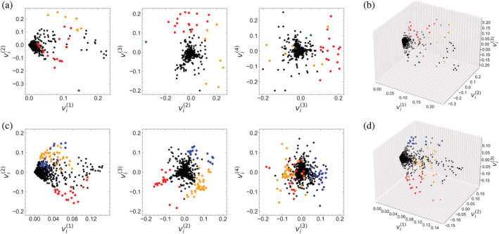
Residue distributions in SVD sequence space. Each point corresponds to one of the $20\ell$ residues of the HD (a,b) or Ras (c,d) MSAs. Values are the elements of the residue eigenvectors (Equation 5). Although scaling these values by their corresponding values would weigh the relative contribution of residues to the sequence alignment, plotting unscaled values gives the direct contribution of each residue in a sequence to the corresponding value (Figure 5). Colored points indicate residues that have frequencies within a k‐means cluster enriched by 0.4 or greater compared to out‐of‐cluster residue frequencies, and represent a sequence signature for that particular cluster. Colors are the same as in Figure 7. To visualize the 3D plots from different angles, see Videos S3 and S4. MSA, multiple sequence alignment; SVD, singular value decomposition

Unlike the sequences, there is no obvious clustering of residues in SVD space (compare Figures 7 and 8). However, the $v_i^{\left(k\right)}$ values determine the ${\sigma }_k{u}_i^{\left(k\right)}$ values (Equation (2)), thus, the distribution of the former should reflect that of the later. To determine which $v_i^{\left(k\right)}$ residue values are responsible for cluster positioning, the MSA can be partitioned by cluster identity and the fraction of each residue at each position can be determined for each cluster. Comparing residue frequencies between different clusters reveals residues that are enriched in each cluster. The $v_i^{\left(k\right)}$ values of these residues are likely to give sequence clusters their unique ${\sigma }_k{u}_i^{\left(k\right)}$ values.

Residues that have high frequencies in one of the four clusters of HD and Ras are colored in Figure 8, using cluster colors from Figure 7. These residues tend to populate the extreme vertices the, $v_i^{\left(2\right)}$, $v_i^{\left(3\right)}$ plane. As expected, residues that are enriched in a particular cluster are generally in the same direction as the ${\sigma }_2{u}_i^{\left(2\right)}$, ${\sigma }_3{u}_i^{\left(3\right)}$ values of sequences in the same cluster (Figure S10).

8. RELATIONSHIP OF SEQUENCE CLUSTERS TO SEQUENCE AND SPECIES PHYLOGENY

The clustering of ${\sigma }_k{u}_i^{\left(k\right)}$ values in SVD space (Figure 7) suggests that the MSA comprises multiple subfamilies. Subfamily structure within a group of sequences is typically identified by constructing a phylogenetic tree, where phylogeny is inferred directly from the protein sequences being analyzed. Such sequence‐based trees are expected to be related to SVD clusters, since both methods use the same information.

Sequence trees for HD and Ras are shown in Figure 9a,b, with cluster identities colored as in Figure 7. At the local level, sequences from the same SVD cluster tend to group together. For Ras, this grouping extends over the entire red cluster, which forms a single, large contiguous block (Figure 9b); likewise, the orange and blue Ras clusters form more‐or‐less contiguous blocks. In contrast, the green Ras cluster is broken up, separating the red, blue, and orange blocks. This distribution reflects the distribution of the four sequence ${\sigma }_k{u}_i^{\left(k\right)}$ clusters in the first three dimensions of SVD space, which is roughly tripodal in shape (Figure 7c,d). The red, orange, and blue clusters form the legs of the tripod and are distinct from one another (as in the sequence tree), each connecting directly to the green cluster at the vertex.

FIGURE 9.

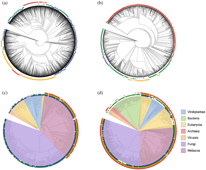
Phylogenetic trees and their relation to SVD clusters. (a,b) Sequence trees of sequences in the HD and Ras MSAs, respectively. (c,d) Species trees of sequences in the HD and Ras MSAs, respectively. Colored marks on the outside of each tree indicate cluster identities using the color scheme in Figure 7. For the species trees, color wedges on the inside indicate major taxa. Sequence trees were generated in MAFFT ²⁹ using default settings. Species trees were generated from PhyloT (https://phylot.biobyte.de/), using the UniProt IDs associated with each sequence in Pfam. Note that there are fewer sequences on the species trees (310 and 430 for HD and Ras, respectively) than on the sequence trees (4,995 and 10,265 for HD and Ras, respectively) because only sequences from organisms with unique UniProt IDs can be depicted. Trees were rendered using iTOL. ³⁰ MSA, multiple sequence alignment; SVD, singular value decomposition

In contrast, the HD sequence tree (Figure 9a) shows considerable mixing of SVD clusters, especially the blue and the green clusters. Sequences in the orange SVD cluster are tightly grouped, although they are interrupted by a block of sequences form the red group, which is itself broken up into two blocks at opposite ends of the tree. Although the blue and green clusters are not cleanly segregated in SVD space, consistent with their mixing on the sequence tree, the red and orange clusters are, yet they are interspersed on the sequence tree. Thus, it seems that some sequence features revealed by SVD differ from those used to construct the tree.

Another way to generate trees from a set of sequences is to use established taxonomies of the organisms from which the sequences derive. We generated such species trees (Figure 9c,d) with PhyloT (https://phylot.biobyte.de/). Although sequence‐ and species‐trees are related, the terminal nodes of species trees (which represent individual species), can contain multiple sequences (Figure 9c,d), whereas those of sequence‐based trees have only one sequence each (Figure 9a,b). One evolutionary mechanism that results in sequence multiplicity involves gene duplication and neofunctionalization under selective pressure, followed by genetic drift. This generates two distinct families of paralogous sequences, which would be separated from each other in a sequence tree (and likely in SVD space), but would be shared in the clades of a species tree.

Paralogous sequences are seen for both HD and Ras (Figure 9c,d). For HD, the blue cluster shows the broadest distribution, and is found in nearly all of the species that could be identified by PhyloT. These species include metazoans, fungi, viridiplantae, and other eukaryotes including amoebozoans and protozoans. The green cluster is also found in most fungi and metazoans, suggesting a paralogous relationship with blue cluster sequences, although it is sparsely represented in plants and other eukaryotes. In contrast, the orange and red clusters are limited exclusively to metazoans, suggesting that these HDs are associated with the HOX genes, which determine the body plan of segmented animals. ¹⁵ Taken together, this distribution suggests that sequences in the blue cluster represent an ancestral HD form, whereas those from the orange and red clusters are more recent adaptations.

For Ras, the green cluster is most broadly distributed, and is found in most species identified by phyloT including metazoans, fungi, viridiplantae, and in a large number of bacterial species. ²⁶ The red cluster is densely distributed across all eukaryotes but is not found in bacteria. The orange and blue clusters are found in metazoans and yeast, but are largely absent from plants and some other eukaryotes. This distribution suggests that sequences from the green cluster form an ancestral lineage, sequences from the red cluster represent a paralogous group that diverged early in the eukaryotic lineage, and sequences from the orange and blue clusters represent paralogous groups that diverged more recently.

Comparison of the distribution of deep ancestral and more recent paralogue clusters shows some shared features for HD and Ras. First, clusters of putative ancestors (blue for HD, green for Ras) are located near the origin of the ${\sigma }_2{u}_i^{\left(2\right)}$, ${\sigma }_3{u}_i^{\left(3\right)}$ plane, whereas other more taxonomically restricted clusters (red and orange for HD, red, orange, and blue for Ras) are at more extreme values of ${\sigma }_2{u}_i^{\left(2\right)}$ and/or ${\sigma }_3{u}_i^{\left(3\right)}$ (Figure 7). Second, for both HD and Ras, the recent paralogue clusters appear to have larger ${\sigma }_1{u}_i^{\left(1\right)}$ values than the ancestral clusters, suggesting a greater degree of sequence variation among ancestral sequences. This type of effect may also arise from a difference in the numbers of ancestral versus recent paralogue clusters and/or a difference in length as described above. The observation that paralogous groups are resolved in the first few dimensions of SVD space is consistent with a mathematical analysis of PCA of phylogenetically related protein sequence subgroups.

9. MAPPING FUNCTIONAL ATTRIBUTES INTO SINGULAR VALUE DECOMPOSITION SPACE

If the sequence clusters in SVD space represent paralogues, sequences in each cluster might be expected to have different functional properties. This can be examined by identifying specific biochemical activities for sequences that are either within the MSA or homologous to MSA sequences, and projecting these sequences into SVD space. If sequences with a particular activity all project to a particular cluster, the whole of that cluster can be considered to represent sequences with that activity. This type of mapping would enable functional annotation of sequences within the cluster that have not been characterized, and would reveal residues that contribute specific functions using the approach described above.

For HD sequences, the DNA specificities of the 84 HDs in Drosophila melanogaster have been determined and have been divided into 11 specificity groups. ²¹ We took the sequences from each of these groups, aligned them with our HD MSA, and projected them into SVD space using Equation (3). The two largest families, which contain the engrailed and antennapedia genes, project into multiple clusters: engrailed projects to the green, yellow, and red (but not blue) clusters, whereas antennapedia projects to the green and yellow (but not red or blue) clusters (not shown). In contrast, sequences from the remaining groups project primarily into a single cluster (Figure 10a,b). Interestingly, only the Six, TGIF, and Iroquois families (which together have been categorized as “atypical” ²¹ ) project to the putative ancestral blue cluster, suggesting these genes may represent ancestral families.

FIGURE 10.

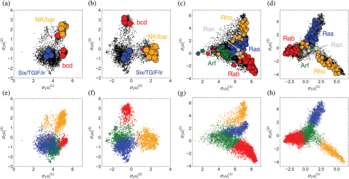
Mapping functional features into SVD space. Projection of sequences with known HD DNA binding specificities (a,b) and Ras‐family specializations (c,d) into SVD space. Projected sequences are colored according to clusters from Figure 7, which are reproduced (e–h) for comparison, and colored black in the projections to contrast the projected sequences. For both protein families, projected sequences segregate to a particular cluster, indicating that these clusters represent specific functional groups. SVD, singular value decomposition

An even stronger functional segregation pattern is seen for Ras. Using a classification scheme that assigns sequences to various subcellular processes, ²⁵ we find that sequences classified to the Rho, Rab, and Ras subfamilies map to the three projections in the, ${\sigma }_2{u}_i^{\left(2\right)}$, ${\sigma }_3{u}_i^{\left(3\right)}$ plot (yellow, red, and blue clusters, respectively, Figure 10). Sequences in the Arf subfamily map to the putative ancestral green cluster at the vertex, whereas Ran sequences map to the intersection between Arf and Rab. Combined with the taxonomic analysis above, this suggests that Rab‐associated vesicular transport ²⁵ was an early adaptation in the eukaryotic lineage. In contrast, the actin regulation associated with the Rho proteins and the transmembrane signaling and gene regulation pathways controlled by the Ras proteins was a more recent adaptation.

10. SCRIPTS FOR SINGULAR VALUE DECOMPOSITION ANALYSIS

Python scripts for SVD analysis of MSAs are available at GitHub (https://github.com/barricklab-at-jhu/SVD-of-MSAs, Appendix S3). These scripts are combined in a single Jupyter notebook that, given an MSA, performs all steps in preprocessing, SVD, and downstream analysis, generating most of the plots presented here (Figure S11).

AUTHOR CONTRIBUTIONS

Autum Koenigs: Conceptualization (equal); data curation (equal); formal analysis (equal); investigation (equal); methodology (equal); resources (equal); software (supporting); validation (equal); visualization (supporting); writing – review and editing (equal). Gina El Nesr: Conceptualization (equal); data curation (equal); formal analysis (equal); investigation (equal); methodology (equal); software (equal); validation (equal); writing – review and editing (equal). Doug Barrick: Conceptualization (equal); formal analysis (equal); funding acquisition (lead); investigation (equal); methodology (equal); project administration (equal); software (equal); supervision (equal); validation (equal); visualization (equal); writing – original draft (lead); writing – review and editing (equal).

CONFLICTS OF INTEREST

The authors state no conflicts of interest.

Supporting information

Appendix S1 Supporting Information

Appendix S2 Supporting information

Baxter‐Koenigs AR, El Nesr G, Barrick D. Singular value decomposition of protein sequences as a method to visualize sequence and residue space. Protein Science. 2022;31(10):e4422. 10.1002/pro.4422

DATA AVAILABILITY STATEMENT

The multiple sequence alignments and python programs used to perform SVD and analyze data are freely available on Github at https://github.com/barricklab-at-jhu/SVD-of-MSAs

REFERENCES

- 1. Ekeberg M, Lövkvist C, Lan Y, Weigt M, Aurell E. Improved contact prediction in proteins: Using pseudolikelihoods to infer Potts models. Phys Rev E Stat Nonlin Soft Matter Phys. 2013;87(1):012707. 10.1103/PhysRevE.87.012707. [DOI] [PubMed] [Google Scholar]
- 2. Morcos F, Pagnani A, Lunt B, et al. Direct‐coupling analysis of residue coevolution captures native contacts across many protein families. Proc Natl Acad Sci U S A. 2011;108(49):E1293–E1301. 10.1073/pnas.1111471108. [DOI] [PMC free article] [PubMed] [Google Scholar]
- 3. Russ WP, Figliuzzi M, Stocker C, et al. An evolution‐based model for designing Chorismate mutase enzymes. Science. 2020;369(6502):440–445. 10.1126/science.aba3304. [DOI] [PubMed] [Google Scholar]
- 4. Halabi N, Rivoire O, Leibler S, Ranganathan R. Protein sectors: Evolutionary units of three‐dimensional structure. Cell. 2009;138(4):774–786. 10.1016/j.cell.2009.07.038. [DOI] [PMC free article] [PubMed] [Google Scholar]
- 5. Rivoire O, Reynolds KA, Ranganathan R. Evolution‐based functional decomposition of proteins. PLoS Comput Biol. 2016;12(6):e1004817. 10.1371/journal.pcbi.1004817. [DOI] [PMC free article] [PubMed] [Google Scholar]
- 6. Hannachi A, Jolliffe IT, Stephenson DB, Trendafilov N. In search of simple structures in climate: Simplifying EOFs. Int J Climatol. 2006;26(1):7–28. 10.1002/joc.1243. [DOI] [Google Scholar]
- 7. Jombart T, Devillard S, Balloux F. Discriminant analysis of principal components: A new method for the analysis of genetically structured populations. BMC Genet. 2010;11(1):94. 10.1186/1471-2156-11-94. [DOI] [PMC free article] [PubMed] [Google Scholar]
- 8. Menozzi P, Piazza A, Cavalli‐Sforza L. Synthetic maps of human gene frequencies in Europeans. Science. 1978;201(4358):786–792. 10.1126/science.356262. [DOI] [PubMed] [Google Scholar]
- 9. Novembre J, Stephens M. Interpreting principal component analyses of spatial population genetic variation. Nat Genet. 2008;40(5):646–649. 10.1038/ng.139. [DOI] [PMC free article] [PubMed] [Google Scholar]
- 10. Reich D, Price AL, Patterson N. Principal component analysis of genetic data. Nat Genet. 2008;40(5):491–492. 10.1038/ng0508-491. [DOI] [PubMed] [Google Scholar]
- 11. Casari G, Sander C, Valencia A. A method to predict functional residues in proteins. Nat Struct Biol. 1995;2(2):171–178. 10.1038/nsb0295-171. [DOI] [PubMed] [Google Scholar]
- 12. Gogos A, Jantz D, Sentürker S, Richardson D, Dizdaroglu M, Clarke ND. Assignment of enzyme substrate specificity by principal component analysis of aligned protein sequences: An experimental test using DNA glycosylase homologs. Proteins. 2000;40(1):98–105. . [DOI] [PubMed] [Google Scholar]
- 13. Waterhouse AM, Procter JB, Martin DMA, Clamp M, Barton GJ. Jalview version 2—A multiple sequence alignment editor and analysis workbench. Bioinformatics. 2009;25(9):1189–1191. 10.1093/bioinformatics/btp033. [DOI] [PMC free article] [PubMed] [Google Scholar]
- 14. Bürglin TR, Affolter M. Homeodomain proteins: An update. Chromosoma. 2016;125:497–521. 10.1007/s00412-015-0543-8. [DOI] [PMC free article] [PubMed] [Google Scholar]
- 15. Carroll S. Homeotic genes and the evolution of arthropods and chordates. Nature. 1995;376:479–485. 10.1038/376479A0. [DOI] [PubMed] [Google Scholar]
- 16. Gehring WJ, Affolter M, Bürglin T. Homeodomain proteins. Annu Rev Biochem. 1994;63:487–526. 10.1146/annurev.bi.63.070194.002415. [DOI] [PubMed] [Google Scholar]
- 17. Banachewicz W, Religa TL, Schaeffer RD, Daggett V, Fersht AR. Malleability of folding intermediates in the homeodomain superfamily. Proc Natl Acad Sci U S A. 2011;108(14):5596–5601. 10.1073/pnas.1101752108. [DOI] [PMC free article] [PubMed] [Google Scholar]
- 18. Carra JH, Privalov PL. Energetics of folding and DNA binding of the MAT alpha 2 homeodomain. Biochemistry. 1997;36(3):526–535. 10.1021/bi962206b. [DOI] [PubMed] [Google Scholar]
- 19. Dragan AI, Li Z, Makeyeva EN, et al. Forces driving the binding of homeodomains to DNA. Biochemistry. 2006;45(1):141–151. 10.1021/bi051705m. [DOI] [PubMed] [Google Scholar]
- 20. Mayor U, Johnson CM, Daggett V, Fersht AR. Protein folding and unfolding in microseconds to nanoseconds by experiment and simulation. Proc Natl Acad Sci U S A. 2000;97(25):13518–13522. 10.1073/pnas.250473497. [DOI] [PMC free article] [PubMed] [Google Scholar]
- 21. Noyes MB, Christensen RG, Wakabayashi A, Stormo GD, Brodsky MH, Wolfe SA. Analysis of homeodomain specificities allows the family‐wide prediction of preferred recognition sites. Cell. 2008;133(7):1277–1289. 10.1016/j.cell.2008.05.023. [DOI] [PMC free article] [PubMed] [Google Scholar]
- 22. Sternke M, Tripp KW, Barrick D. Consensus sequence design as a general strategy to create hyperstable, biologically active proteins. Proc Natl Acad Sci U S A. 2019;116:11275–11284. 10.1073/pnas.1816707116. [DOI] [PMC free article] [PubMed] [Google Scholar]
- 23. Sternke M, Tripp KW, Barrick D. Surface residues and nonadditive interactions stabilize a consensus homeodomain protein. Biophys J. 2021;120:5267–5278. [DOI] [PMC free article] [PubMed] [Google Scholar]
- 24. Tripp KW, Sternke M, Majumdar A, Barrick D. Creating a homeodomain with high stability and DNA binding affinity by sequence averaging. J Am Chem Soc. 2017;139:5051–5060. 10.1021/jacs.6b11323. [DOI] [PMC free article] [PubMed] [Google Scholar]
- 25. Rojas AM, Fuentes G, Rausell A, Valencia A. The Ras protein superfamily: Evolutionary tree and role of conserved amino acids. J Cell Biol. 2012;196(2):189–201. 10.1083/jcb.201103008. [DOI] [PMC free article] [PubMed] [Google Scholar]
- 26. Wuichet K, Søgaard‐Andersen L. Evolution and diversity of the Ras superfamily of small GTPases in prokaryotes. Genome Biol Evol. 2015;7(1):57–70. 10.1093/gbe/evu264. [DOI] [PMC free article] [PubMed] [Google Scholar]
- 27. Sternke M, Tripp KW, Barrick D. Chapter seven: The use of consensus sequence information to engineer stability and activity in proteins. In: Tawfik DS, editor. Enzyme engineering and evolution: General methods. Methods in enzymology. Volume 643. Cambridge: Academic Press, 2020; p. 149–179. 10.1016/bs.mie.2020.06.001. [DOI] [PMC free article] [PubMed] [Google Scholar]
- 28. Mistry J, Chuguransky S, Williams L, et al. Pfam: The protein families database in 2021. Nucleic Acids Res. 2021;49(D1):D412–D419. 10.1093/nar/gkaa913. [DOI] [PMC free article] [PubMed] [Google Scholar]
- 29. Katoh K, Misawa K, Kuma K‐i, Miyata T. MAFFT: A novel method for rapid multiple sequence alignment based on fast Fourier transform. Nucleic Acids Res. 2002;30(14):3059–3066. 10.1093/nar/gkf436. [DOI] [PMC free article] [PubMed] [Google Scholar]
- 30. Letunic I, Bork P. Interactive tree of life (ITOL) v5: An online tool for phylogenetic tree display and annotation. Nucleic Acids Res. 2021;49(W1):W293–W296. 10.1093/nar/gkab301. [DOI] [PMC free article] [PubMed] [Google Scholar]
- 31. Qin C, Colwell LJ. Power law tails in phylogenetic systems. Proc Natl Acad Sci U S A. 2018;115(4):690–695. 10.1073/pnas.1711913115. [DOI] [PMC free article] [PubMed] [Google Scholar]
Associated Data
This section collects any data citations, data availability statements, or supplementary materials included in this article.
Supplementary Materials