EHHR: an efficient evolutionary hyper-heuristic based recommender framework for short-text classifier selection

Abstract

With various machine learning heuristics, it becomes difficult to choose an appropriate heuristic to classify short-text emerging from various social media sources in the form of tweets and reviews. The No Free Lunch theorem asserts that no heuristic applies to all problems indiscriminately. Regardless of their success, the available classifier recommendation algorithms only deal with numeric data. To cater to these limitations, an umbrella classifier recommender must determine the best heuristic for short-text data. This paper presents an efficient reminisce-enabled classifier recommender framework to recommend a heuristic for new short-text data classification. The proposed framework, “Efficient Evolutionary Hyper-heuristic based Recommender Framework for Short-text Classifier Selection (EHHR),” reuses the previous solutions to predict the performance of various heuristics for an unseen problem. The Hybrid Adaptive Genetic Algorithm (HAGA) in EHHR facilitates dataset-level feature optimization and performance prediction. HAGA reveals that the influential features for recommending the best short-text heuristic are the average entropy, mean length of the word string, adjective variation, verb variation II, and average hard examples. The experimental results show that HAGA is 80% more accurate when compared to the standard Genetic Algorithm (GA). Additionally, EHHR clusters datasets and rank heuristics cluster-wise. EHHR clusters 9 out of 10 problems correctly.

Introduction

Recent efforts in machine learning (ML) focus on automation of the heuristic selection process by incorporating domain independence [1]. The search techniques for selecting heuristics are generalized by making the search process independent of the considered domain. However, the heuristic approaches and other search strategies in solving real-world computational search issues are challenging in freshly-discovered and new instances of the same problem. Such problems arise from various parameters, algorithm choices, and the absence of selection criteria [2]. Hyper-heuristics approaches are generic and domain-independent to search and solve a problem set rather than a single problem. These approaches target a heuristic search space instead of a solution search space. These approaches have been extensively researched in timetabling, bin packing, data mining, and feature selection [3]. However, their application for classifier selection in the domain of short-text data has not been paid much attention. Short-text is an important source of data from online platforms like microblogs, e-commerce systems, and social networks, in the form of comments, tweets, and reviews [4, 5]. It is called short-text as fewer characters are used to provide what people think, such as a tweet can have a maximum of 280 characters. Various industries analyze the social media-generated comments and user feedback by using ML approaches to identify problems, elicit requirements [6], provide interest-based recommendations [7], improve their products and services for the end users [8, 9].

Varying backgrounds, language usage, and writing styles of social media users instigate the lexical, syntactic, and semantic (language morphology) perplexity of short-text, thus contributing to the diversity of such data [10]. In addition, since most words appear only once and there are not enough contexts to clarify the meaning of ambiguous words, short-text experiences severe data sparsity problems compared to long text [11, 12]. The key problem with short-text classification is the brevity of the short-text and the sparsity of the feature space [13]. Various statistical, Machine Learning (ML), and Deep Learning (DL)-based heuristics have been developed to classify task-specific short-text data [14–21]. In accordance with the “No Free Lunch theory [22, 23],” there is no single heuristic that works best for all short-text classification problems. Brute force search of the best classifier for such big short-text data is expensive yet impractical in terms of time and computational resource utilization [24]. Additionally, selecting an acceptable heuristic for addressing a short-text classification problem is not simple since the problem’s features are typically not well understood in advance [25]. In this context, how to automatically recommend the best heuristic is a major concern for classifying a short-text problem at hand, especially for non-experts [26, 27]. Although, existing research focused on classifier recommendations. However, they only deal with numeric or categorical data [1, 28, 29]. Some of the meta-learning-based techniques [30, 31] utilize the human expert opinion for recommending the best classifier on numeric data. Motivated by these concerns, it is inevitable to determine the best heuristic for classifying a short-text dataset and conserving the computational resources, especially for high volume, sparse, and diverse short-text datasets.

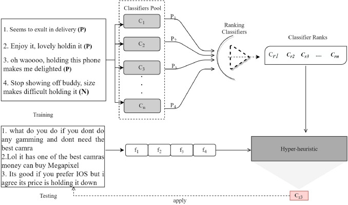
This paper aims to develop a hyper-heuristic framework (see  Fig.1) to recommend the best short-text classifier. Figure 1 depicts the working of the classifier recommender. Classifiers’ from the classifiers pools are executed on the training datasets to achieve their relative performances and rank and reminisce them. The hyper-heuristic uses dataset-level features of the test dataset to predict performance and recommend the best classifier based on the reminisced classifier ranking. The framework is intended to make an intelligent choice of a machine learning classifier less time-consuming by reusing the performances of heuristics on previously solved problems. Equipped with Feature Extraction Module (FEM), Heuristic Evaluation Module (HEM), Evolutionary Module (EM), and Memory Module (MM), the proposed Evolutionary Hyper-heuristic based Recommender Framework (EHHR) saves and reminisces the performance of different classifiers for various datasets. The EHHR employs an evolutionary algorithm called Hybrid Adaptive Genetic Algorithm (HAGA), which serves as a hyper-heuristic. HAGA contributes to determining the most influential dataset-level features and performance prediction. Based on the predicted performance, the ranks of classifiers are determined through a clustering algorithm.

Fig. 1.

Handling of classifier selection problem through Hyper-heuristic. $C_{\mathit{ri}}$ is classifier’s rank, $f_i$ are dataset-level features. $P_i$ is the performance of classifier $C_i$. $C_{r3}$ is the best-predicted classifier for testing the dataset

Contributions of the study

The contribution of this study is three-fold. It recommends the best-suited classifier for short-text data from a heuristic space (i.e., a pool of classifiers). It also determines the best dataset-level features playing an important role in choosing the best classifier. It minimizes the need for a stochastic search of classifiers for a dataset and automates the choice of the best classifier. The following are the major contributions of this paper.

• A novel Hyper-Heuristic Classifier Recommender (EHHR) to automatically recommend the best heuristic for the short-text classification is proposed.

• A Hybrid Adaptive Genetic Algorithm (HAGA) for determining the most influential dataset-level features in EHHR, is proposed.

• A new framework is presented to investigate the performance of heuristics for the large volume, varying sized, balanced, and imbalanced data.

• A reminisce-enabled model has been devised to minimize the need for the stochastic search for the most suitable classifier for an unseen dataset.

The rest of the paper is organized as follows. Section 2 presents the related work to highlight the gaps in the previous studies. The modules and operations of the proposed technique have been discussed in detail in Sect. 3. In the Sect. 4, we provide the details of the experimental setup. Section 5 contains detailed results and analysis. Section 6 concludes the study.

Related work

Heuristic techniques have been widely applied to perform data classification tasks [32, 33]. A heuristic for one dataset may not be equally effective for another dataset [34]. Moreover, they are expensive due to their problem-specific nature [2] and lose their generality due to customization and parameter tuning. Different studies focused on recommending an appropriate heuristic (i.e., an appropriate classifier), which is answered in the context of the numeric form of data, as discussed ahead.

Pise and Kulkarni [35] used simple, information-theoretic, and statistical meta-features for algorithm selection. To recommend the best algorithm, the suggested technique used the K-Nearest Neighbor (KNN) algorithm and the classifier’s accuracy as the recommendation measure. The experiment indicates that calculated accuracies match actual accuracies for over 90% of the benchmark datasets used. However, the approach suffers from computation overload due to the inefficient selection of meta-features, which results in calculating all meta-features. The classifier selection for real-time intrusion detection [36] necessitates a tedious re-evaluation process resulting from changing classifiers.

The study [28] uses real-coding evolutionary algorithm to present Automatic Machine Learning (Auto-ML) based solution for automatic classifier recommendation. Statistical and structural information-based method of feature vector generation using KNN [37] only works with binary data sets and cannot discriminate between the target and other characteristics. Furthermore, calculating itemset frequency for high-dimensional data takes more time and space. Wang’s classifier recommendation [38] technique is based on extracting attribute correlations from the data set’s structure but results in high computational costs for itemset generation. Link prediction through DAR (Data and Algorithm Relationship) Network [39] suffers from the choice of optimal value for k (which remained fixed for all datasets). CB-MLR [31] and AMD [30] need human experts’ involvement in defining application-specific goals and for empirical evaluation of classifiers’ performance based on quality meta-metrics, respectively.

The EML (i.e., Ensemble of ML-KNN ) is a two-layer-recommendation technique that uses diverse meta-features and KNN to measure similarity between predicted and archived problems. However, setting an appropriate K value requires expert knowledge [26]. Li et al. [29] proposed a meta-learning-based technique for solving engineering problems in manufacturing systems. The framework proposed dataset, classifier algorithm, and recommendation modules to suggest several algorithms for a dataset. However, the technique heavily relied on an accurate selection of hit rate and accuracy to avoid misleading recommendations of an algorithm. Corrales et al. [40] proposed an algorithm recommender for regression and classification problems using case-based reasoning. The limitation of the system lies in that the efficiency declines when there is an increase in search time for similar solved cases.

To make an appropriate classifier recommendation, an important aspect is to achieve it through domain independence of the problem, which is mainly realized using hyper-heuristic approaches. Evolutionary techniques have demonstrated their significance as hyper-heuristic techniques for problem areas such as bin-packing [41], image segmentation [42], timetabling [43]. Hyper-heuristic (HH) has been used in a variety of fields, especially with classification problems [44]. The major issue with these approaches is that they only apply to specific problems and do not store and reuse the previously solved problems to guide the search of heuristics for the unseen instances. To overcome this issue, the Deja Vu framework maintains an Acquired Knowledge Module(AKM) to store problem definitions, fitness functions, and best-performing heuristics for each problem [1]. The framework solves the new problem based on similarity to an existing problem. Though the framework has been tested with various classification problems, it does not apply to text categorization problems due to text data’s unstructured nature. Hence, the requirement of a hyper-heuristic to tackle the classifier recommendation of short-text for balanced, imbalanced, and voluminous datasets arises.

The above-mentioned techniques work with numeric and categorical data (i.e., see Table 13in Appendix A). The meta-learning techniques lack the optimization of features, resulting in computational and memory overhead. Furthermore, some of them introduce a high reliance on human expertise. To the best of our knowledge, no classifier recommendation has been presented to date to cater to the needs of short-text data.

Table 13.

Comparison of EHHR with state-of-the-art

Technique	Data			Domain	Methodology	Reminisce
	Type	Size	Category
EHHR	T	H, M	B,I	Short-text	HH	Y
[35]	N, C	S	I	Multiple	Mtl	Y
[64]	N, C	S	I	Multiple	Mtl	Y
[36]	N	M	I	Network IDS	Empirical	N
[28]	N, C	S	I	Imageaudio	Mtl	N
[1]	N C	S, M	I	Multiple	HH	Y
[37]	N, C	S, M	I	Multiple	Mtl	Y
[38]	N, C	S	I		Mtl	Y
[39]	N, C	S, M	I	Multiple	Mtl	Y
[31]	N, C	S	I	Multiple	Mtl	Y
[65]	N	S	I	Multiple	HH	N
[66]	N, C	S, M	I	Multiple	Mtl	Y
[67]	N, C	S	I	Multiple	Mtl	N
[30]	N,C	S	I	Multiple	Mtl	N
[68]	N	M	I	IoT	Mtl	Y
[26]	N	M	I	Multiple	Mtl	Y
[29]	N,C	S,M	I	Multiple	Mtl	Y

Proposed technique

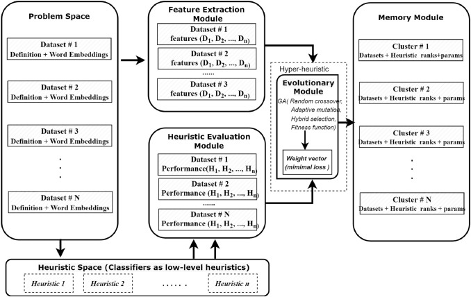
The proposed Evolutionary Hyper-Heuristic Classifier Recommender (EHHR) framework intends to determine the ranking of the various heuristics based on their performance in classifying short-text data. This framework comprises four segments: Feature Extraction Module (FEM), Heuristic Evaluation Module, Evolutionary Module, and Memory Module. These segments contain dataset features, a list of heuristics with their parameter settings, and heuristics’ performance for each dataset. Figure 2 shows the functioning and interaction of the modules of the EHHR framework. Data originating from various data sources is preprocessed and then input to the FEM, which calculates the 18 features for each dataset. The heuristic evaluation module of the EHHR framework computes the performance of multiple heuristics for each dataset. The heuristic space comprises a set of classifiers which are in the Classifier Pool in Fig. 1. The evolutionary module of EHHR optimizes and predicts the most influential dataset features and the average classifier performance. The heuristic performances help to group datasets into clusters and predict their ranking. The memory module stores the clusters’ information and heuristics’ ranking along with their best parameter values. This information is reminisced to recommend the best classifier for a new problem.

Fig. 2.

The proposed framework of EHHR for short-text data

Feature extraction module (FEM)

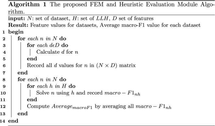
FEM facilitates the computation of the linguistic complexity of a dataset. It computes different dataset-level features for the problem domain N to compute the linguistic complexity. These features belong to lexical, syntactic, or word length categories (reference Table 1). Lexical measures help the framework evaluate the lexicon’s worth in text and use lexical sophistication and lexical variation measures. Syntactic measures are computed through syntactic complexity indices, and the readability scores quantify the complexity of short-text in terms of reading ease. It produces a feature set matrix (NxD dimensions) as shown in algorithm 1, where D is dataset-level features, and N represents a dataset in the problem space. Explanation of the features, taken from the literature [10, 45–50] is provided in Appendix B with respect to types and token.

Table 1.

Features for datasets linguistic complexity analysis in FEM

Category	Reference	Feature
Syntactic complexity indices	[10]	Mean length of Sentence (MLS)
Lexical sophistication	[48]	LS1
		LS2
Lexical variation	[48]	Lexical word variation
		Verb variation-II (VV-2)
		Noun variation (NV)
		Adjective Variation (AdjV)
		Type–token ratio (TTR)
		Uber index
Lexical Diversity	[46]	Measure of Textual Lexical Diversity (MTLD)
Lexical richness	[49]	Hapax Richness
Lexical readability	[45]	Flesch-kincaid readability score
		Flesch’s reading ease score
Spelling mistakes	[50]	Percentage of spelling mistakes
Word length	[47]	Mean Length of Word Strings

Proposed features

Along with the features presented in table 1, we also developed the following features for our framework.

1. Percentage of Hard examples: Hard examples refer to the instances in the dataset incorrectly labeled by the classifier [51]. We have taken all the misclassified examples as the hard examples. For example, if the model misclassifies 20 examples for a dataset of 100 examples, then the 20 examples are considered hard examples. The percentage of hard examples($H_p$) is used as a descriptor in EHHR. The ratio of the total number of misclassified examples ($E_m$) by a classifier to the total number of instances in the training sample ($E_t$) provides $H_p$ (i.e., see Eq. 1).

   $$\begin{array}{c}\hfill H_p=\frac{E_m}{E_t}\ast 100\end{array}$$ 1
2. Average Entropy of frequently occurring words: The average entropy of the most frequent words is computed for each dataset. The average entropy measures the informational value contributed by the frequently occurring words in the dataset according to the Eq. 2. $w_j$ is a word type in W, n is the total number of words in the corpus, also known as vocabulary size, while $prob(w_j)$ is the probability of $w_j$ in the corpus. $prob(w_j)$ is the ratio of the frequency of $w_j$ to the sum of all type frequencies within n. f is the number of frequent words.

   $$\begin{array}{c}\hfill E_{\mathit{avg}}=\frac{1}{f}[-\sum _{j=1}^n(logprob(w_j)\ast lo{g}_{2}prob(w_j))]\end{array}$$ 2
3. Average TF-IDF: Average TF-IDF is the mean of TF-IDF values of the most frequent words. The average values help to quantify the central tendency of the most relevant words in the short-text. If $Y_i$ represents the TF-IDF value of a word $x_i$ $ϵ$ X, and f is the number of top frequent words. Then the average TF-IDF is calculated as presented in Eq. 3:

   $$\begin{array}{c}\hfill AverageTF-IDF=\frac{1}{f}[\sum _{i=1}^f(Y_i)]\end{array}$$ 3

Heuristic evaluation module

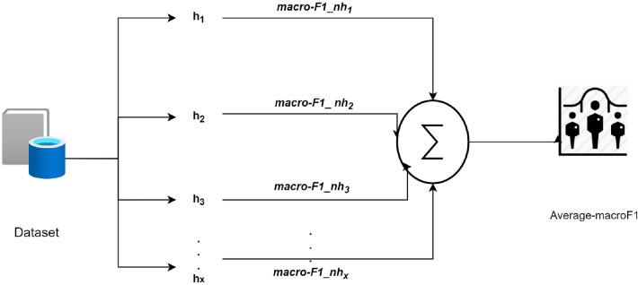
The heuristic evaluation module unmasks the actual performance of heuristics (i.e., see Fig. 3) for problems being considered. The heuristic space of the proposed framework comprises a pool of state-of-the-art classification algorithms. Each heuristic h from the heuristic search space H is trained on (the embeddings for) each dataset n from the set of datasets N, and its actual performance is calculated as shown in algorithm 1 (lines 8–13). The proposed algorithm uses macro f1-score as the performance measure. Generally, the recommendation frameworks use accuracy as a performance measure. However, the proposed framework used macro f1-score, which is a good predictor for varying sized and highly skewed (i.e., imbalanced) datasets. Algorithm 1 computes the heuristic evaluation vector (Nx1 dimensions).

Fig. 3.

The heuristic evaluation process in EHHR resulting in computation of actual performance in terms of average macro-F1 for each dataset n $ϵ$ N

The average macro f1-score of all heuristics in H for each dataset is computed and recorded. The heuristic evaluation is only applied during the training phase of the framework and is computationally expensive. However, these computations serve as the basis for the reminiscence (i.e., recalling the classifier’s past performances) and re-usability of the low-level heuristic’s previously-stored performances to solve new problems. Furthermore, the module saves the best parameter values for all heuristics. For a dataset n $ϵ$ N, the f1-score ($macroF{1}_{n{h}_i}$) is computed for each $h_i$. The Eq. 4 presents the calculation of the average macro f1-score for all heuristics for each dataset.

$$\begin{array}{c}\hfill Averag{e}_{macroF1}=\frac{1}{z}[\sum _{i=1}^z(macroF{1}_{n{h}_i})]\end{array}$$ 4

In Eq. 4, $h_i$ refers to heuristic and n is the dataset. Variable i is used to iterate through 1 to z, where z is the total number of heuristics in the heuristic space.

Evolutionary module

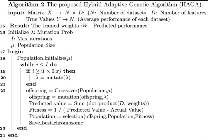
In the evolutionary module, the proposed Hybrid Adaptive Evolutionary Algorithm (HAGA) is trained to predict the average performance for the given data. HAGA is an improvement to the general GA applied in a hyper-heuristic setting. For a population of $\mu$ chromosomes, the selection process of HAGA is the hybridization of tournament selection with elitism. To cater to the problem of a less diverse population and premature convergence arising due to elitism, some chromosomes are randomly selected for the new population. Furthermore, the adaptive mutation and random crossover in HAGA encourage the exploration of global optimum and population diversity. In the training phase, HAGA takes the extracted features (explained in Section Feature Extraction Module (FEM)) as input data and the actual average performances of the classifiers for each data as true values. The average macro f1-score (computed in the heuristic evaluation module) is the true label for training the HAGA.

The chromosomes of the HAGA contain the weights for the input features. The weights are multiplied by the features and summed up. The output value presents the predicted average performance. The fitness function of HAGA is a minimization function that evolves the weights in order to minimize the loss. The difference between the predicted and actual performance is taken as the loss. The actual performance is the average performance of each dataset w.r.t. macro f1-score. Equation 5 computes the average loss for all datasets.

$$\begin{array}{c}\hfill \text{Average Loss}=\frac{1}{n}\left(\sum _{i=1}^n,(predicte{d}_i-actua{l}_i)\right)\end{array}$$ 5

The detailed pseudo-code for the HAGA is given in Algorithm 2. The convergence (very low update in loss) of the HAGA is considered the termination criteria. The key differences between the basic GA and the proposed HAGA are given below:

1. Mutation value is adaptive. Mutation rate changes after every x% of iterations instead of fixed mutation value.

2. Hybrid selection strategy has been applied for selecting chromosomes for the next generation.

3. The crossover point is not fixed; we select random points for each crossover to ensure diversity in the population.

The output of the HAGA is the weight vector that best minimizes the loss. In the testing phase, for any given dataset, the features vector ($N\times 1$) is multiplied by the weight vector. It returns the predicted average performance of that dataset. For any given dataset, the average performance will be predicted using HAGA rather than the training of the machine learning classifiers.

Memory module

The memory module of EHHR stores the results produced by all modules and clustering algorithms to reminisce them for new datasets. The EHHR uses a fuzzy C-means clustering algorithm to cluster datasets. The primary objective of the clustering process is to decrease the dissimilarity between the data allocated within the same cluster [52]. Clustering is a technique that can group classifiers with similar performances within the same cluster to minimize the complexity of predicting one or more classifiers to a user. Fuzzy c-means (FCM) is a type of clustering technique in which it is possible to cluster values that lie in two or more clusters with similar degrees of membership without any difficulty [53]. Hence, this module groups the datasets into clusters based on their performances.

The memory module stores the obtained clusters of datasets based on performance, with best-performing heuristics and their parameter settings obtained during the training phase. Each cluster provides the ranking of low-level heuristics.

Handling an unseen problem

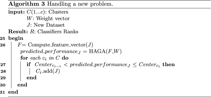
EHHR helps determine the best classifier for a new problem without stochastically running all heuristics. First, the features presented in Section Feature Extraction Module (FEM) are extracted for the new dataset. These features are used to predict the performance with the help of HAGA. The cluster is assigned to the dataset based on the predicted performance. The best algorithm for the chosen cluster is applied to the new problem. The memory module is updated with the extracted feature values and the chosen heuristic of the new dataset (i.e., see Algo. 3). The reason for performing clustering is that it will provide the ranks of algorithms based on the performance of the classifiers for different datasets. When a new problem is encountered, EHHR predicts the performance using HAGA instead of running all classifiers. HAGA reuses the average performances of classifiers on previously solved problems to predict the performance of an unseen dataset. Later, a cluster is assigned to this unseen dataset based on predicted average performance for the recommendation of an ML classifier. The time spent collectively executing HAGA and clustering for an unknown dataset is significantly less than executing and evaluating individual classifiers on that dataset. It chooses a classifier that is less time-consuming for a short-text dataset.

For cluster assignment to the unseen/test data, the euclidean distance is calculated between the centroid of the clusters and the predicted performance of the unseen dataset. The euclidean distance $d(u_i,c_i)$ (i.e., see Eq. 6) is the square root of the sum of the squares of the differences between the predicted performance ($u_i$) of unseen dataset and cluster centroid ($c_i$) in each dimension [54]. The dataset is assigned the cluster for which the distance is minimum.

$$\begin{array}{c}\hfill d(u_i,c_i)=\sqrt{{(u_i-c_i)}^2}\end{array}$$ 6

Example of EHHR

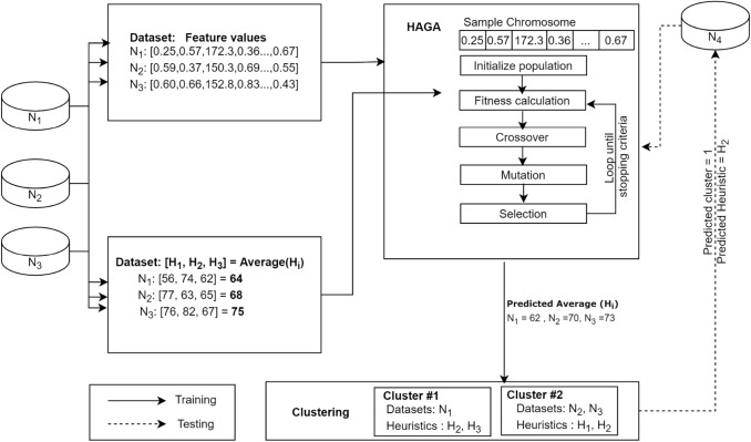
Figure 4 provides an example of EHHR application on three sample datasets $N_1$, $N_2$ and $N_3$. $H_i$ shows the heuristics and the classifier algorithms in the heuristic space. The FEM module computes feature values for the datasets. The heuristic evaluation module computes the performances of the classifiers for each dataset. For example, the average performance of $H_1$, $H_2$, $H_3$ is 64 for $N_1$ dataset. The computed performances and features are used by the HAGA to predict the average performance for all datasets using feature values. The next step involves the clustering of the datasets based on performance. In the test case, HAGA predicts the performance of heuristics using features for a test dataset. Clusters are assigned to the test dataset (for example, $N_4$) based on HAGA prediction.

Fig. 4.

An example of training and testing in EHHR

Materials and methods

This section provides the experimentation details for the proposed EHHR framework.

Experimental setup

This section presents the experimental setup and parameter settings for the framework. Section 4.1.1 explains the dataset used and its experimental settings. Section 4.1.2 provides embedding and their setup.

Benchmark datasets and preprocessing

All the experiments were carried out on ten balanced and imbalanced short-text datasets. Jigsaw comment and Landslide datasets have been collected from UCI [55] and the GRAIT-DM project [56], respectively. All the remaining datasets have been collected from Kaggle [57]. These datasets contain short-text reviews, tweets, or SMS. Table 2 provides the datasets’ details, including the size and percentage of positive and negative examples. Sentiment140 and IMDB datasets contain an equal distribution of positive and negative examples. Landslide, Jigsaw comments, DrugsCom, Amazon baby reviews, Google playstore reviews, and Women clothing datasets depict high skewness in data distribution.

Table 2.

The short-text datasets and their respective percentages of positive-negative instances

S #	Dataset	# of instances	Positive %	Negative
1	Sentiment140 (S)	1.6 million	50	50
2	Jigsaw toxic comments (J)	312,735	7	65
3	Landslide (L)	282,152	83	17
4	DrugsCom (D)	215,063	75	25
5	Amazon baby reviews (A)	183,531	76	14
6	IMDB movie reviews (I)	50,000	50	50
7	Google playstore reviews (G)	64,295	74	26
8	Coronavirus_archive (C)	46,162	41	59
9	Reddit data (R)	37,249	43	35
10	Women clothing ecommerce (W)	23,486	82	18

The datasets were modified and cleaned as a first step in the framework. Multiclass datasets were mapped to binary classes. The examples with neutral sentiment labels were removed for the multiclass datasets, such as Google playstore data. The reviews and rating columns for the datasets, such as DrugCom, were retrieved. We manually observed the samples to consider them either low for lower satisfaction levels or high for higher satisfaction. We took a random sample of 200 examples for binary classification and analyzed the comments. The rating values in the dataset were in the range of 1–10. By observing the user comments, it was found that 1–4 rating comments were not good, so we considered them low ratings (i.e., 0-label). Since the remarks with a rating of 5–10 seemed favorable, we assigned them a high rating (1-label). The general text cleaning tasks included the removal of punctuation marks, HTML tags, and stopwords. In addition, each dataset was preprocessed using case conversion and lemmatization procedures.

Word embedding

EHHR was evaluated with two different models ($EHH{R}_{\mathit{BERT}}$ and $EHH{R}_{\mathit{TfIdf}}$) based on word embeddings (BERT and TF-IDF). For $EHH{R}_{\mathit{BERT}}$, the word embedding of each dataset was extracted through the pre-trained model of BERT${}_{\mathit{BASE}}$ (Bidirectional Encoder Representations from Transformers) model  [58]. BERT${}_{\mathit{BASE}}$ architecture contains 12 encoder layers, 768 hidden layers, and 12 attention heads. The BERT provides embeddings of each word with 768 dimensions. The bidirectional nature of BERT allowed the framework to learn the lexicon of words in the short-text corpus. Hence, BERT provided a deeper understanding of word perspective than sequential models. The machine learning classifiers were added atop the CLS tokenś transformer output.$EHH{R}_{\mathit{TfIdf}}$ was implemented by extracting word embedding Term Frequency-Inverse Document Frequency (TF-IDF) technique. It is a numerical statistic designed to represent the significance of a word in a collection or corpus of documents  [59]. BERT takes roughly 5 min for a chunk of 5000 examples. The smallest data contain (Reddit) 17k examples; BERT extracted the embeddings of that data in 17 min. The largest data (Sentiment) contains 16m examples. BERT takes 1600 min to extract the embedding of that data. The execution time of ML classifiers depends on the parameter setting and is data-dependent. The running time of HAGA is 40 min. Clustering takes 0.0064 s.

Features extraction

The purpose of the FEM is to find out the features presented in Sect. 3.1 for each dataset. Each dataset was passed to the FEM to extract the features. Lexically sophisticated features of each short-text dataset were retrieved with the help of lexical tokens. For calculating lexical variation descriptor, BNC (British National Corpus) wordlist [60] served as a basis to determine the verb, noun, and adjective types in tweets, comments, and reviews in the datasets. The BNC list contains 29 different families of words retrieved from British and American English to assist vocabulary analysis of the text.

The readability tests were calculated with two variables: average sentence length and average word length. The IMDB dataset showed the highest reading ease score, while DrugCom scored the lowest. For calculating the percentage of hard examples in each dataset, a neural network was set up with 100 hidden layer elements, 0.0001 value for regularization parameter, and a constant learning rate. The top 50 frequently occurring words in each short-text dataset were retrieved to compute the average entropy of frequent items. The sample size for calculating the average TFIDF values was also specified as 50 most frequent words for each dataset.

Heuristics and parameter setting

The heuristic space of EHHR used Support Vector Machine (SVM), K Nearest Neighbour (KNN), Random Forest (RF), Gaussian Naive Bayes (GNB), Decision Tree (DT), and Neural Network (NN) were chosen as Machine Learning (ML) heuristic models. To implement and execute these models, we used Scikit-learn, numpy, and panda python libraries. All datasets were evaluated for the same parameter settings of ML models. Each dataset was split into 70 ratios, 30 for training and testing tasks. The parameters are trained using the grid search strategy. The details of heuristic-wise parameters are given in Table 3. KNN classifier is executed for k range between 3 and 31 (i.e., with a step-size 2). We have used a fully-connected feed-forward NN that takes BERT or TFIDF embedding as an input. NN is searched with tanh, relu, and logistic activations, along with lbfgs, sgd, and adam sovlers for weight optimization. NN shows the best performance for the combination of Rectified Linear Unit (relu) and Stochastic Gradient Descent (sgd) with 0.001 L2 penalty and 0.001 learning rate for both versions of EHHR. RF and DT are tested with a depth range of 4 to 64.

Table 3.

Heuristic’s parameters and their values

Heuristic	Parameter	Value
KNN	K	3–13 with step-size =2
DT, RF	Depth	4–64
NN	Hidden layer sizes	(128,64))
	solver	lbfgs, sgd, adam
	activation	tanh, relu,logistic
SVM	Kernel	Linear

Results and discussion

This section presents the results obtained from the experiments and their discussion.

Heuristic space

As explained in Sect. 4.1.4, the heuristic space of EHHR used SVM, KNN, RF, GNB, DT, and NN. Table 4 shows the best parameter values achieved for each model. For KNN, K=3 turned out to be the best parameter setting for the majority of the datasets in the case of $EHH{R}_{\mathit{BERT}}$ and $EHH{R}_{\mathit{TfIdf}}$ (i.e., see Table 4). NN shows the best performance for the combination of Rectified Linear Unit (relu) and Stochastic Gradient Descent (sgd) with 0.001 L2 penalty and 0.001 learning rate for both versions of EHHR. RF depicts its best performance for tree depths equal to 16 and 32 for $EHH{R}_{\mathit{BERT}}$ and $EHH{R}_{\mathit{TfIdf}}$, respectively. The best tree depths for DT are 32 and 64 with entropy selection measures for $EHH{R}_{\mathit{BERT}}$ and $EHH{R}_{\mathit{TfIdf}}$ respectively.

Table 4.

Best parameter values achieved for each heuristic in the heuristic space

Heuristic	Parameter	Best value
		$EHH{R}_{\mathit{BERT}}$	$EHH{R}_{\mathit{TfIdf}}$
KNN	K	3	3
DT	Depth	32	64
	Criteria	Entropy	Entropy
RF	Depth	16	32
	Criteria	Entropy	Entropy
	n-estimators	200	200
NN	Hidden layer sizes	(128,64)	(128,64)
	solver	sgd	sgd
	activation	relu	relu
	Learning rate	0.001	0.001
SVM	Kernel	Linear	Linear
	C	1	1

Comparison of EHHR model using TFIDF and BERT embeddings

Table 5 provides heuristic’s macro f1-score (i.e., first row) and micro f1-score (i.e., second row) achieved for each dataset for the best values of parameters with $EHH{R}_{\mathit{BERT}}$. The average performance of all heuristics for each dataset is the highest for the Landslide dataset (i.e., equal to 92% for macro f1-score). The Women clothing dataset achieves a 64% average performance, which shows that it is difficult to predict compared to other datasets. The difference between the heuristic’s average micro and average macro f1-scores remains below 4% for Reddit, IMDB, Corona tweets, and Sentiment140 datasets. It is because the training sample fairly represents the positive and negative classes. The difference between the heuristic’s average micro and macro f1-score is significant for the remaining datasets. The differences arise as the micro and macro f1-scores are calculated differently. The micro f1-score assigns equal weight to each sample, and the macro f1-score assigns equal weight to each class. Table 5 also demonstrates the average performance of heuristics in terms of macro and micro f1-scores for all datasets. Neural Network outperforms other used heuristics in terms of macro and micro f1-score. The macro f1-score-based performance of NN is in a range of 4–23% better as compared to other heuristics. The performance of SVM is similar to RF. The micro f1 score for RF is better than DT, SVM, KNN, and GNB within a range of 2–16%. GNB performance in macro f1-score is less than all other heuristics for all datasets except the Sentiment140 dataset.

Table 5.

Best performance values achieved for each heuristic in terms of Macro f1 (first row) and Micro f1-score (second row) for $EHH{R}_{\mathit{BERT}}$

Dataset	DT	RF	SVM	NN	KNN	GNB	Average
Reddit	67	77	82	84	73	63	74
	68	77	82	84	74	64	75
Women Clothing	59	58	76	73	54	37	60
	75	84	83	86	79	37	74
IMDB	61	69	75	79	61	52	66
	61	69	75	79	61	62	68
Google Playstore	75	78	75	79	67	52	71
	81	80	78	84	76	76	79
Corona tweets	61	67	66	69	62	56	64
	62	70	67	70	65	63	66
Jigsaw comments	67	75	72	80	66	44	67
	67	93	78	94	90	90	85
Amazon baby dataset	60	63	74	78	56	53	64
	78	86	82	84	83	68	80
Drugs	80	85	70	76	60	49	70
	84	90	78	84	72	53	77
Landslide	95	97	94	95	87	85	92
	95	97	94	97	95	76	92
Sentiment140	57	66	69	72	67	64	66
	57	66	69	72	67	58	65
Macro f1-score	68	74	75	79	65	56
Micro f1-score	73	81	79	83	76	65

Table 6 provides the performances of heuristics for datasets with the best values of parameters using $EHH{R}_{TF-IDF}$. The average performance of all the heuristics on the Landslide dataset is high. The Sentiment140 dataset is proven to be complex data for most heuristics. The heuristic’s performance on the Women Clothing dataset is similar to the Sentiment140 dataset. In the case of TFIDF-based embedding, both datasets are difficult to predict. The difference between the heuristic’s average micro and average macro f1-scores remains below 3% for Reddit, IMDB, Corona tweets, Google Playstore, Landslide, and Sentiment140 datasets. For the remaining datasets, this difference is above 6%. The performance of the KNN heuristic is acceptable only on Drugs and Jigsaw datasets. In contrast, the performance of GNB is poor on Drugs and Jigsaw-comments datasets. Macro f1-score of NN is better than other heuristics in a range of 2–18%. On the other hand, the micro-f1-based performance of SVM is highest, i.e., in a range of 1–13%.

Table 6.

Best performance values achieved for each heuristic in terms of Macro f1 (first row) and Micro f1-score (second row) for $EHH{R}_{\mathit{TfIdf}}$

Dataset	DT	RF	SVM	NN	KNN	GNB	Average
Reddit	85	85	87	84	53	81	79
	85	85	87	84	57	81	80
Women Clothing	65	70	76	76	63	69	70
	78	86	88	86	81	76	83
IMDB	67	80	83	82	65	80	76
	67	80	83	82	65	80	76
Google Playstore	80	85	85	89	63	75	80
	83	88	89	92	65	78	83
Corona tweets	75	77	75	75	60	71	72
	77	79	78	76	66	72	75
Jigsaw comments	65	70	74	77	71	62	70
	83	87	92	93	91	76	87
Amazon baby dataset	70	76	80	78	60	70	72
	81	86	91	79	83	78	83
Drugs	80	85	73	88	75	68	78
	84	90	82	91	83	72	84
Landslide	97	96	94	99	67	89	90
	97	96	95	99	67	90	91
Sentiment140	67	68	72	71	67	70	69
	68	69	72	71	67	70	70
Macro f1-score	75	79	80	82	64	74
Micro f1-score	80	85	86	85	73	77

Tables 5 and 6 show that NN model performs better than other models for both TFIDF and BERT-based embedding. From the point of view of datasets, on average, the performances of the heuristics on the Landslide dataset are better compared to other datasets. In the case of TFIDF, the performance of SVM and RF models is comparable to that of NN. It is because SVM performs effectively in high-dimensional space (i.e., embedding is high-dimensional). Moreover, the tree ensembling strategy of RF minimizes the overfitting and provides improved performance [61, 62]. The difference in performances of heuristics on different datasets strongly supports the theory of “No Free Lunch” [23]. The theorem asserts that no heuristic consistently performs well across all datasets. Furthermore, there are different skewness levels for each dataset. Thus, heuristics become biased when training with the imbalanced dataset [63]. The average performance of the five heuristics across all datasets is superior for TFIDF than for BERT. The only exception is the KNN algorithm which shows better results with BERT embedding. However, only the KNN algorithm exhibits better performance with BERT-based embedding.

Performance of the evolutionary module

The HAGA’s (i.e., see Sect. 3.3) application on datasets helped predict the average performance of a classifier. The HAGA chromosome is an 18-dimensional vector, where each gene represents a feature (i.e., from 18 features) of each dataset (see Table 7). All the features are normalized within a range of 0 and 1 and serve as genes of a chromosome. The number of maximum iterations is kept very large to ensure that convergence should be achieved before reaching the maximum iterations. In the worst case (no convergence), the maximum number of iterations will be served as the termination criteria. The loss value for each dataset is calculated by subtracting the actual average macro f1-score from the predicted average macro f1-score (i.e., see Eq. 5). The Final Loss value achieved is 1.9, with a standard deviation of 0.3. Hence, the HAGA can predict the average macro f1-score with an error margin of 1.5 to 2.3. Therefore, without training, we can predict the performance with marginal error. Furthermore, this reduces the time for the choice of the classifier for a problem and helps overcome the brute force searching of heuristics for a new problem.

Table 7.

A training sample for the evolutionary module. Average macro-F1 is the average F1 scores of all heuristics for each dataset

N	TTR	MLWS	UI	MTLD	HR	LS1	LS2	.	AE	TFIDF	macro-F1
N${}_1$	0.36	5.11	26.4	174.9	0.21	0.32	0.48	.	0.07	0.05	68
N${}_2$	0.23	4.07	24	81.1	0.14	0.4	0.58	.	0.1	0.07	73
N${}_3$	0.56	7.82	42	378.8	0.42	0.68	0.67	.	0.04	0.04	79
.	.	.	.	.	.	.	.	.	.	.	.
N${}_n$	0.44	5.01	21.8	104.39	0.24	0.30	0.4	.	0.08	0.03	56

Influential features predicted by HAGA

The HAGA in the EHHR framework also predicts the importance of the features of the dataset. The table 8 shows the importance score for the top five features. The importance score validates the dataset descriptors presented in section FEM. The highest importance score achieved by the average entropy proves it is the most important descriptor of data for solving DT and RF algorithms. The variety in verbs and adjectives has also been among the top five descriptors. The number of hard examples can facilitate determining the complexity of various datasets and the effect of data complexity on the classifier’s performance.

Table 8.

Top five important descriptors with their importance scores

S #	Feature	Importance score
1	Average Entropy	0.24
2	Mean Length of Word String	0.20
3	Adjective Variation	0.19
4	Verb Variation  II	0.15
5	Hard Examples	0.05

Convergence of the HAGA

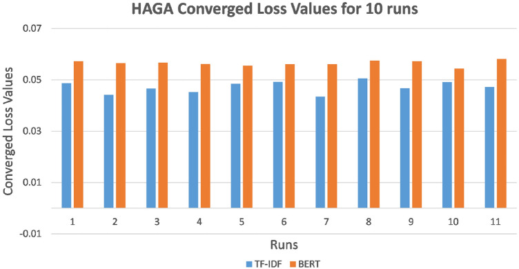
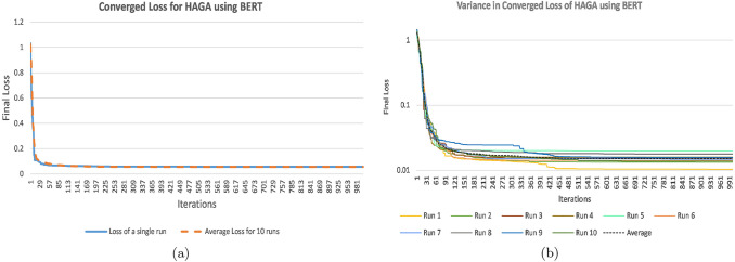
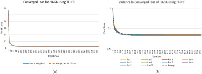
To validate the performance of the HAGA, the experiments were run ten times. Figure 5 shows the finally converged values for loss achieved for each run. The difference in converged loss value in ten runs remained within a range of 0.055 to 0.059 in case of BERT-based embedding, resulting in minute difference of 0.004. For TFIDF, the difference range was 0.045 -0.050. The difference in final loss computed during each run of HAGA in $EHH{R}_{\mathit{BERT}}$ is less than the final loss to HAGA in $EHH{R}_{\mathit{TFIDF}}$. Figures 6a and 7a show the comparison of convergence of HAGA between a single run and the average of multiple runs. The x-axis shows the number of iterations, and the y-axis depicts the loss values reached in each iteration. The closeness of the two series in both graphs validates the persistent performance of the proposed technique. Furthermore, Figs. 6b and 7b depict the variance on a logarithmic scale among ten different runs of HAGA using BERT-based and TFIDF-based EHHR, respectively. We show that the variance between multiple runs is small, which shows the consistency of the proposed technique.

Fig. 5.

Converged loss values for ten runs of HAGA

Fig. 6.

Convergence of the HAGA in $EHH{R}_{\mathit{BERT}}$ a Final Loss for single run compared to the final loss of average of ten runs, b Variation in final loss for ten different runs and the final loss of average of ten runs

Fig. 7.

Convergence of the HAGA in $EHH{R}_{\mathit{TFIDF}}$ a Final Loss for single run compared to the final loss of average of ten runs, b Variation in final loss for ten different runs and the final loss of average of ten runs

Correlation among influential features

The heatmap presented in the Fig. 8 shows the correlation among the five most influential features. The smaller correlation value between $H_p$ and $E_{\mathit{avg}}$ shows the weak linear relationship between the percentage of hard examples and the average entropy of the frequent words in short-text data. The correlation between the VV-II and AdjV is 0.52, which confirms that both are positively correlated and influential in determining the class of a sample in short-text data. MLWS shows a negative correlation with VV-II and AdjV. The heatmap analysis depicts that 38% of the variation in AdjV is negatively correlated to MLWS, and approximately 8% of the decrease in VV-II is associated with an increase in MLWS. Furthermore, our analysis showed that the two influential features (MLWS and Average Entropy), with the highest importance values, have a strong inverse relationship.

Fig. 8.

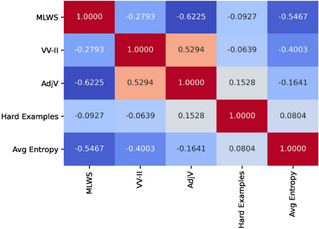
Correlation among the top five influential dataset-level features optimized by HAGA

Comparison of HAGA with standard genetic algorithm

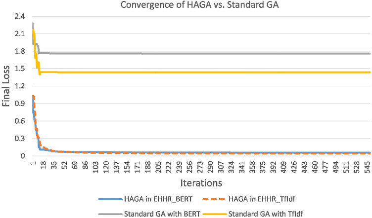
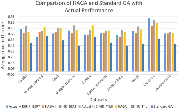
In order to validate the performance of HAGA, it is compared with a standard genetic algorithm. The standard GA is implemented with a single-point crossover, fixed mutation rate of 0.02, and tournament selection strategy. Figure 9 illustrates the final loss values achieved for HAGA for $EHH{R}_{\mathit{BERT}}$ and $EHH{R}_{\mathit{TfIdf}}$ and standard GA over 500 iterations. The standard GA is evaluated for BERT and TFIDF embeddings results. The curves of standard GA in both cases show notably large differences in final loss values. In both models, HAGA’s convergence curves remain below the standard GA’s convergence curve, thus resulting in predicting performance close to the actual performances. Importantly, the overlapping of the curves for HAGA with $EHH{R}_{\mathit{BERT}}$ and $EHH{R}_{\mathit{TfIdf}}$ demonstrates the proposed framework’s consistent performance. Furthermore, due to the adaptive mutation rate, HAGA explores and exploits a diversified population compared to standard GA. Table 9 shows the difference between the performance predicted by a standard GA and the proposed HAGA for both models of EHHR. The predicted performances of HAGA for both models show that HAGA outperforms standard GA in 8 out of 10 datasets (i.e., see Fig. 10).

Fig. 9.

Comparison of HAGA with Standard GA for Converged Loss iterations

Table 9.

Comparison of the actual average macro f1-score with the predicted average macro f1-score of HAGA and standard GA (normalized in the scale of 0-1)

Dataset	Average macro f1-score
	$EHH{R}_{\mathit{BERT}}$		$EHH{R}_{\mathit{TfIdf}}$		Standard GA
	Actual	HAGA	Actual	HAGA
Reddit	0.74	0.67	0.79	0.68	0.49
Women Clothing	0.60	0.69	0.70	0.77	0.61
IMDB	0.66	0.68	0.76	0.75	0.54
Google Playstore	0.71	0.67	0.80	0.72	0.44
Corona	0.64	0.64	0.72	0.80	0.60
Jigsaw toxic comments	0.67	0.67	0.70	0.71	0.50
Amazon baby dataset	0.64	0.60	0.72	0.68	0.45
Drugs	0.70	0.67	0.78	0.73	0.48
Landslide	0.92	0.79	0.90	0.84	0.57
Sentiment140	0.66	0.66	0.69	0.67	0.48

Fig. 10.

Comparison of actual average macro f1-score for each dataset to the predicted average macro f1-score of HAGA and Standard GA

Data clustering

After applying the fuzzy C-means clustering, two clusters have been identified. In the case of $EHH{R}_{\mathit{BERT}}$, the clusters are generated with an average macro f1-score greater than 68% (i.e., for cluster 1) and less than or equal to 68% (i.e., cluster 2). Table 10a and b show the heuristic’ ranking for each cluster for $EHH{R}_{\mathit{BERT}}$. Table 11a and b display the heuristic’ ranking for each cluster for $EHH{R}_{\mathit{TfIdf}}$. In the case of $EHH{R}_{\mathit{TfIdf}}$, the clusters are obtained with cluster centers at 78.79% and 70.62%. The ranks are computed based on the macro f1-score performance. “Actual” is the cluster assigned to the dataset based on actual performance, while “Predicted” refers to the cluster assigned to the dataset based on the predicted performance obtained by the proposed model. The clusters obtained from the predicted performance are similar to those obtained from actual performances in both versions of EHHR, except for the IMDB dataset as shown in Table 12. These results verify that EHHR performance remains equally good when different embedding are used.

Table 10.

Cluster-wise heuristic ranks for $EHH{R}_{\mathit{BERT}}$

(a) Cluster 1		(b) Cluster 2
Rank	Algorithm	Rank	Algorithm
1	NN	1	NN
1	RF	2	SVM
2	SVM	3	RF
2	DT	4	DT
4	KNN	4	KNN
5	GNB	5	GNB

Table 11.

Cluster-wise heuristic ranks for $EHH{R}_{\mathit{TfIdf}}$

(a) Cluster 1		(b) Cluster 2
Rank	Algorithm	Rank	Algorithm
1	NN	1	NN
2	RF	1	SVM
3	DT	2	RF
4	SVM	3	DT
5	GNB	3	GNB
6	KNN	4	KNN

Table 12.

Dataset clusters based on actual and predicted performance

Dataset	$EHH{R}_{\mathit{BERT}}$		$EHH{R}_{\mathit{TfIdf}}$
	Actual	Predicted	Actual	Predicted
Reddit	1	1	1	1
Women Clothing	2	2	2	2
IMDB	1	2	2	1
Google Playstore	1	1	1	1
Corona	2	2	2	2
Jigsaw toxic comments	2	2	2	2
Amazon baby dataset	2	2	2	2
Drugs	1	1	1	1
Landslide	1	1	1	1
Sentiment140	2	2	2	2

The research findings indicate that EHHR performs similarly for different word embedding and can effectively anticipate the best-performing short-text classification heuristic. An important advantage of the EHHR is that it uses a high-level strategy with little or no technical knowledge of low-level heuristics. In contrast to expert opinion-dependent techniques [30, 31], EHHR predicts the best heuristic for short-text classification automatically, thus minimizing the need for human involvement. Unlike the techniques proposed in [26, 29], EHHR does not heavily rely on an accurate selection of features and parameters for evaluation. As EHHR uses the previously solved problems to guide the search for the best heuristic for short-text, enabling the heuristic prediction to be less time-consuming. However, the heuristic evaluation module needs to execute all heuristics for classifying short-text data only once.

Conclusion and future work

Choosing a classification heuristic is important when applying a classifier to a new dataset or new instances of an existing dataset. Additionally, the heuristics’ performance varies per problem. The existing research provides the solution to the abovementioned problem for numeric data. However, a classifier recommendation mechanism that exists for short-text data is lacking. The paper overcomes this limitation for short-text datasets with the help of hyper-heuristic. It presents a framework with feature extraction, heuristic evaluation, evolutionary and memory modules to calculate and obtain heuristic performances. Furthermore, the memory module stores and reuses the previously solved short-text classification problems. The proposed Evolutionary Hyper-heuristic-based Recommender framework EHHR is evaluated using six different machine learning heuristics and macro f1-score as the performance measure. The Neural network is the best heuristic, achieving 79% and 82% performances with BERT and TFIDF embedding, respectively. The Hybrid Adaptive Genetic Algorithm (HAGA) enables EHHR to identify the most significant dataset-level traits and achieves an 80% accuracy rate in performance prediction. HAGA reveals that average entropy, mean length of the word string, adjective variation, verb variation II, and average hard examples are the top five influential features for predicting average performance. The datasets are clustered based on the average performance. The EHHR with TFIDF and BERT-based embedding predict consistently correct clusters for 9 out of 10 datasets based on the predicted performance by HAGA.

In the future, we want to add and evaluate more short-text datasets from different domains such as biology and software engineering to our framework. It will aid in broadening the scope of EHHR’s applicability to other domains.

Biographies

Bushra Almas

is a Ph.D. student at National University of Computer and Emerging Sciences (NUCES), Pakistan. She is presently working as Assistant Professor at Quaid-i-Azam University, Islamabad. Her research interests include Data Mining, Machine Learning, and Big Data Analytics.

Hasan Mujtaba

is Professor at National University of Computer and Emerging Sciences, Islamabad since 2010. He did his Post Doctorate from University of Nottingham (2013) and was associated ASAP Research Group. His research interests are in the areas of Artificial Intelligence, Computational Intelligence, Machine Learning, Data Mining & Knowledge Discovery, Evolutionary Gaming, and Machine Vision & Robotics. He is actively involved in research in these areas and has several publications to his name.

Kifayat Ullah Khan

is working as an Associate Professor in Department of Computer Science. His research interests include Data Warehousing, Data Mining, Social Networks Analysis, Graph Summarization, Artificial Intelligence, Internet of Things, and Big Data. He has several publications in the form of patents, journals, and conferences of prestige, including some research works currently in progress/review. He is an active researcher and working on various research assignments/projects in collaboration with researchers from different national and international institutes.

Appendix A Comparison of EHHR with state-of-the-art

The dataset types can either be Numeric(N) or Categorical(C) or Text (T). “Category” is either Balanced (B) or Imbalanced (I). The “Methodology” used to perform each techniques is categorized as Meta-learning (Mtl) or Hyper-Heuristic (HH) as shown in Table 13.

Appendix B Explanation of features in FEM

The symbols used in formulae are: the number of word types(W), sophisticated words ($W_p$), lexical words ($W_{\mathit{lx}}$, sophisticated lexical words ($W_{\mathit{plx}}$, verbs ($W_{\mathit{vb}}$), sophisticated verbs ($W_{\mathit{svb}}$, nouns ($W_{\mathit{noun}}$ , adjectives ($W_{\mathit{adj}}$ for word types; and, the number of word tokens (X), lexical words ($X_{\mathit{lx}}$), sophisticated lexical words ($X_{\mathit{slx}}$), verbs ($X_{\mathit{verb}}$) considering the word tokens. Sophisticated refers to the advanced, content-bearing terms that are not commonly used in writing [69].

B.1 Syntactic complexity indices

EHHR considers Mean length of Sentence (MLS) in order to measure the syntactic complexity of dataset. Mean Length of Sentence (MLS): As the focus of this study is short-text datasets, the production length at sentence-level is considered as one of the feature to be utilized in the framework. It is computed (i.e., see Eq. B1) as the ratio of count of words (i.e. tokens) to the sentence count in the corpus to (S).

$$\begin{array}{c}\hfill MLS=\frac{X}{S}\end{array}$$ B1

B.2 Lexical sophistication

The percentage of unconventional words in the data refers to the Lexical sophistication. Lexical sophistication 1 and 2 are computed for datasets in EHHR.

1. LS1: LS1 is calculated as the ratio between the measure of $W_{\mathit{slx}}$ (sophisticated lexical words) to $W_{\mathit{lx}}$ (i.e., total lexical words, Eq. B2 ).

   $$\begin{array}{c}\hfill LS1=\frac{W_p}{W}\end{array}$$ B2
2. LS2: The proportion of the count of sophisticated word types($X_s$) to count of word types (X) as presented in Eq B3.

   $$\begin{array}{c}\hfill LS2=\frac{X_{\mathit{slx}}}{X_{\mathit{lx}}}\end{array}$$ B3

B.3 Lexical variation

For computing the extent of vocabulary usage is calculated with the help of lexical variation of words, verbs, nouns and adjective in the dataset.

1. Lexical word variation (LWV): Lexical Word Variation (Eq. B4) is obtained by calculating the percentage of lexical word type count to total lexical words count.

   $$\begin{array}{c}\hfill LWV=\frac{W_{\mathit{lx}}}{X_{\mathit{lx}}}\end{array}$$ B4
2. Verb variation-II (VV-2): It is calculated as the ratio between the count of verb types count to the total verbs count in a short-text (Eq. B5).

   $$\begin{array}{c}\hfill VV-2=\frac{W_{\mathit{vb}}}{X_{\mathit{lx}}}\end{array}$$ B5
3. Noun variation (NV): The ratio of nouns usage in writer’s comments to the lexical words in corpus(Eq. B6).

   $$\begin{array}{c}\hfill NV=\frac{W_{\mathit{noun}}}{X_{\mathit{lx}}}\end{array}$$ B6
4. Adjective Variation (AdjV): It is the ratio of adjectives used in writer’s comments to the lexical words in corpus (Eq. B7). It is important to note that the use of adjectives make a short-text positive or negative.

   $$\begin{array}{c}\hfill AdjV=\frac{W_{\mathit{adj}}}{X_{\mathit{lx}}}\end{array}$$ B7
5. Type-token ratio (TTR): Type–token ratio (TTR) is obtained by dividing the number of word types by the number of words present in the text (Eq. B8). Types are the unique lexical elements used in a corpus.

   $$\begin{array}{c}\hfill TTR=\frac{W}{X}\end{array}$$ B8
6. Uber index: It is a transformation of TTR (Eq. B9).

   $$\begin{array}{c}\hfill \text{Uber Index}=\frac{Lo{g}^{2}X}{Log(X/W)}\end{array}$$ B9

B.4 Lexical diversity

Lexical diversity (LD) measures the vocabulary range adopted in the corpus. Measure of Textual Lexical Diversity (MTLD): MTLD helps to valuate the lexical diversity of the short-text irrelevant to corpus length. It is “the mean length of sequential word strings in a text that maintain a given TTR value” [70].

B.5 Lexical richness

It is the assessment of text richness with the help of lexical diversity measures. Another measure of lexical richness you may use is Hapax richness, defined as the number of words that occur only once divided by the number of total words. To calculate this, simply use a logical operation on the document-feature matrix to return a logical value for each term that occurs once and then sum up the rows to get a count. Last but not least, calculate it as a proportion of the overall number of words (ntokens) for better interpretation within your overall corpora.

Hapax Richness: It determine the proportion once occurring words($R_1$) in the corpus.

$$\begin{array}{c}\hfill \text{Hapax Richness}=\frac{R_1}{X}\end{array}$$ B10

B.6 Lexical readability

The readability of a corpus is quantified keeping in view the length of sentence and words. Two formulae are used in the proposed framework considering mean of number of words in a sentence(i.e. sentence length $L_s$) and average syllables per word (word length $L_w$). The $L_s$ is computed by dividing the number of words by the number of sentences in a corpus. $L_w$ is generated as a result of dividing the number of syllables to the number of words. The coefficients of the reading ease scale involve the systematic selection of word samples from data [71].

1. Flesch-kincaid readability score: The measure is computed using word and sentence length (i.e., see Eq. B11).

   $$\begin{array}{c}\hfill 206.835-1.015(L_s)-84.6(L_W)\end{array}$$ B11
2. Flesch’s reading ease score: This measure (Eq. B12) quantifies a text within the range of 1 (lowest readability of text) and 100 (highest readability).

   $$\begin{array}{c}\hfill 0.39(L_s)+11.8(L_W)-15.59\end{array}$$ B12

B.7 Data quality

Spelling mistakes: Proportion of the misspelled words (M) in the corpus (Eq. B13) is determined to assess the quality of the short-text in the framework.

$$\begin{array}{c}\hfill Spellingmistakes=\frac{M}{X}\end{array}$$ B13

B.8 Word length

Mean Length of Word Strings: It (Eq. B14) is the average syllables per word (word length $L_w$).

$$\begin{array}{c}\hfill L_w=\frac{Totalsyllables}{X}\end{array}$$ B14

Author contributions

All authors contributed to the study conception. Methodology design, data collection, analysis and visualization were performed by BA. The first draft of the manuscript was written by BA and HM and KUK commented on previous versions of the manuscript. All authors read and approved the final manuscript.

Funding

The authors declare that no funds or grants were received during this research.

Data availability

The datasets analysed during the current study are available from the corresponding author on reasonable request.

Code availability

Available

Declarations

Conflict of interest

The authors declare no conflict of interest.

Consent to participate:

Not applicable

References

- 1.Majeed H, Naz S. Deja vu: a hyper heuristic framework with record and recall (2r) modules. Clust. Comput. 2019;22(3):7165–7179. doi: 10.1007/s10586-017-1095-x. [DOI] [Google Scholar]
- 2.Burke EK, Gendreau M, Hyde M, Kendall G, Ochoa G, Özcan E, Qu R. Hyper-heuristics: a survey of the state of the art. J. Oper. Res. Soc. 2013;64(12):1695–1724. doi: 10.1057/jors.2013.71. [DOI] [Google Scholar]
- 3.Montazeri M. Hhfs: Hyper-heuristic feature selection. Intell. Data Anal. 2016;20(4):953–974. doi: 10.3233/IDA-160840. [DOI] [Google Scholar]
- 4.Song G, Ye Y, Du X, Huang X, Bie S. Short text classification: a survey. J. Multimed. 2014;9(5):635. doi: 10.4304/jmm.9.5.635-643. [DOI] [Google Scholar]
- 5.Grida M, Soliman H, Hassan M. Short text mining: state of the art and research opportunities. J. Comput. Sci. 2019;15(10):1450–1460. doi: 10.3844/jcssp.2019.1450.1460. [DOI] [Google Scholar]
- 6.Lafi M, Hawashin B, AlZu’bi S. Eliciting requirements from stakeholders' responses using natural language processing. Comput. Model. Eng. Sci. 2021;127(1):99–116. [Google Scholar]
- 7.Hawashin, B., Mansour, A., Fotouhi, F., AlZu'bi, S., Kanan, T.: A novel recommender system using interest extracting agents and user feedback. In: 2021 International Conference on Information Technology (ICIT), pp. 674--678 (2021). IEEE
- 8.Lin, W., Xu, H., Li, J., Wu, Z., Hu, Z., Chang, V., Wang, J.Z.: Deep-profiling: a deep neural network model for scholarly web user profiling. Cluster Comput. 1-14 (2021)
- 9.Sengupta E, Nagpal R, Mehrotra D, Srivastava G. Problock: a novel approach for fake news detection. Clust. Comput. 2021;24(4):3779–3795. doi: 10.1007/s10586-021-03361-w. [DOI] [PMC free article] [PubMed] [Google Scholar]
- 10.Lu X. Automatic analysis of syntactic complexity in second language writing. Int. J. corpus Linguist. 2010;15(4):474–496. doi: 10.1075/ijcl.15.4.02lu. [DOI] [Google Scholar]
- 11.Nimala K, Jebakumar R. A robust user sentiment biterm topic mixture model based on user aggregation strategy to avoid data sparsity for short text. J. Med. Syst. 2019;43(4):1–13. doi: 10.1007/s10916-019-1225-5. [DOI] [PubMed] [Google Scholar]
- 12.Yao, D., Bi, J., Huang, J., Zhu, J.: A word distributed representation based framework for large-scale short text classification. In: 2015 International Joint Conference on Neural Networks (IJCNN), pp. 1–7 (2015). IEEE
- 13.Alsmadi, I., Gan, K.H.: Review of short-text classification. Int. J. Web Inf. Syst. (2019)
- 14.Zhang H, Zhong G. Improving short text classification by learning vector representations of both words and hidden topics. Knowl.-Based Syst. 2016;102:76–86. doi: 10.1016/j.knosys.2016.03.027. [DOI] [Google Scholar]
- 15.Ali, M., Khalid, S., Rana, M.I., Azhar, F.: A probabilistic framework for short text classification. In: 2018 IEEE 8th Annual Computing and Communication Workshop and Conference (CCWC), pp. 742–747 (2018). 10.1109/CCWC.2018.8301712
- 16.Zeng, J., Li, J., Song, Y., Gao, C., Lyu, M.R., King, I.: Topic memory networks for short text classification. arXiv preprint arXiv:1809.03664 (2018)
- 17.Chen, J., Hu, Y., Liu, J., Xiao, Y., Jiang, H.: Deep short text classification with knowledge powered attention. In: Proceedings of the AAAI Conference on Artificial Intelligence, vol. 33, pp. 6252–6259 (2019)
- 18.Xu J, Cai Y, Wu X, Lei X, Huang Q, Leung H-F, Li Q. Incorporating context-relevant concepts into convolutional neural networks for short text classification. Neurocomputing. 2020;386:42–53. doi: 10.1016/j.neucom.2019.08.080. [DOI] [Google Scholar]
- 19.Alsmadi IM, Gan KH. Short text classification using feature enrichment from credible texts. Int. J. Web Eng. Technol. 2020;15(1):59–80. doi: 10.1504/IJWET.2020.107689. [DOI] [Google Scholar]
- 20.Chen W, Xu Z, Zheng X, Yu Q, Luo Y. Research on sentiment classification of online travel review text. Appl. Sci. 2020 doi: 10.3390/app10155275. [DOI] [Google Scholar]
- 21.Niu Y, Zhang H, Li J. A nested chinese restaurant topic model for short texts with document embeddings. Appl. Sci. 2021 doi: 10.3390/app11188708. [DOI] [Google Scholar]
- 22.Adam, S.P., Alexandropoulos, S.-A.N., Pardalos, P.M., Vrahatis, M.N.: No free lunch theorem: a review. In: Approximation and Optimization, pp. 57–82 (2019)
- 23.Wolpert, D.H., Macready, W.G., et al.: No free lunch theorems for search. Technical report, Technical Report SFI-TR-95-02-010, Santa Fe Institute (1995)
- 24.Zuo Y, Wang Y, Laili Y, Liao TW, Tao F. An evolutionary algorithm recommendation method with a case study in flow shop scheduling. Int. J. Adv. Manuf. Technol. 2020;109(3):781–796. doi: 10.1007/s00170-020-05471-y. [DOI] [Google Scholar]
- 25.Fan Q, Jin Y, Wang W, Yan X. A performance-driven multi-algorithm selection strategy for energy consumption optimization of sea-rail intermodal transportation. Swarm Evol. Comput. 2019;44:1–17. doi: 10.1016/j.swevo.2018.11.007. [DOI] [Google Scholar]
- 26.Zhu X, Ying C, Wang J, Li J, Lai X, Wang G. Ensemble of ml-knn for classification algorithm recommendation. Knowl.-Based Syst. 2021;221:106933. doi: 10.1016/j.knosys.2021.106933. [DOI] [Google Scholar]
- 27.Ahmed, F., Ferdows, R., Islam, M.R., Kamal, A.R.M.: Autocl: A visual interactive system for automatic deep learning classifier recommendation based on models performance. arXiv preprint arXiv:2202.11928 (2022)
- 28.de Sá, A.G., Pappa, G.L., Freitas, A.A.: Towards a method for automatically selecting and configuring multi-label classification algorithms. In: Proceedings of the Genetic and Evolutionary Computation Conference Companion, pp. 1125–1132 (2017)
- 29.Li L, Wang Y, Xu Y, Lin K-Y. Meta-learning based industrial intelligence of feature nearest algorithm selection framework for classification problems. J. Manuf. Syst. 2022;62:767–776. doi: 10.1016/j.jmsy.2021.03.007. [DOI] [Google Scholar]
- 30.Ali R, Lee S, Chung TC. Accurate multi-criteria decision making methodology for recommending machine learning algorithm. Expert Syst. Appl. 2017;71:257–278. doi: 10.1016/j.eswa.2016.11.034. [DOI] [Google Scholar]
- 31.Ali, R., Khatak, A.M., Chow, F., Lee, S.: A case-based meta-learning and reasoning framework for classifiers selection. In: Proceedings of the 12th International Conference on Ubiquitous Information Management and Communication, pp. 1–6 (2018)
- 32.Kanan, T., AbedAlghafer, A., Kanaan, G.G., AlShalabi, R., Elbes, M., AlZubi, S.: Arabic text categorization: A comparison survey. In: 2021 International Conference on Information Technology (ICIT), pp. 739–742 (2021). IEEE
- 33.Kanan T, Hawashin B, Alzubi S, Almaita E, Alkhatib A, Maria KA, Elbes M. Improving arabic text classification using p-stemmer. Recent Adv. Comput. Sci. Commun. 2022;15(3):404–411. doi: 10.2174/2666255813999200904114023. [DOI] [Google Scholar]
- 34.Sterkenburg, T.F., Grünwald, P.D.: The no-free-lunch theorems of supervised learning. Synthese 1–37 (2021)
- 35.Pise, N., Kulkarni, P.: Algorithm selection for classification problems. In: 2016 SAI Computing Conference (SAI), pp. 203–211. IEEE (2016)
- 36.Nguyen, H.A., Choi, D.: Application of data mining to network intrusion detection: classifier selection model. In: Asia-Pacific Network Operations and Management Symposium, pp. 399–408. Springer (2008)
- 37.Song Q, Wang G, Wang C. Automatic recommendation of classification algorithms based on data set characteristics. Pattern Recogn. 2012;45(7):2672–2689. doi: 10.1016/j.patcog.2011.12.025. [DOI] [Google Scholar]
- 38.Wang G, Song Q, Zhu X. An improved data characterization method and its application in classification algorithm recommendation. Appl. Intell. 2015;43(4):892–912. doi: 10.1007/s10489-015-0689-3. [DOI] [Google Scholar]
- 39.Zhu X, Yang X, Ying C, Wang G. A new classification algorithm recommendation method based on link prediction. Knowl.-Based Syst. 2018;159:171–185. doi: 10.1016/j.knosys.2018.07.015. [DOI] [Google Scholar]
- 40.Corrales DC, Ledezma A, Corrales JC. A case-based reasoning system for recommendation of data cleaning algorithms in classification and regression tasks. Appl. Soft Comput. 2020;90:106180. doi: 10.1016/j.asoc.2020.106180. [DOI] [Google Scholar]
- 41.López-Camacho E, Terashima-Marin H, Ross P, Ochoa G. A unified hyper-heuristic framework for solving bin packing problems. Expert Syst. Appl. 2014;41(15):6876–6889. doi: 10.1016/j.eswa.2014.04.043. [DOI] [Google Scholar]
- 42.AbdElaziz M, Ewees AA, Oliva D. Hyper-heuristic method for multilevel thresholding image segmentation. Expert Syst. Appl. 2020;146:113201. doi: 10.1016/j.eswa.2020.113201. [DOI] [Google Scholar]
- 43.Raghavjee R, Pillay N. A genetic algorithm selection perturbative hyper-heuristic for solving the school timetabling problem. ORiON. 2015;31(1):39–60. doi: 10.5784/31-1-158. [DOI] [Google Scholar]
- 44.Sabar NR, Ayob M, Kendall G, Qu R. Automatic design of a hyper-heuristic framework with gene expression programming for combinatorial optimization problems. IEEE Trans. Evol. Comput. 2015;19(3):309–325. doi: 10.1109/TEVC.2014.2319051. [DOI] [PubMed] [Google Scholar]
- 45.Campaign, P.E.: How to write in plain english. Plain English Campaign (2004)
- 46.McCarthy, P.M.: An assessment of the range and usefulness of lexical diversity measures and the potential of the measure of textual, lexical diversity (mtld). PhD thesis, The University of Memphis (2005)
- 47.Grzybek, P.: History and methodology of word length studies. In: Contributions to the Science of Text and Language, pp. 15–90. Springer (2007)
- 48.Lu X. The relationship of lexical richness to the quality of esl learners' oral narratives. Mod. Lang. J. 2012;96(2):190–208. doi: 10.1111/j.1540-4781.2011.01232_1.x. [DOI] [Google Scholar]
- 49.Tanaka-Ishii K, Aihara S. Computational constancy measures of texts-yule's k and rényi's entropy. Comput. Linguist. 2015;41(3):481–502. doi: 10.1162/COLI_a_00228. [DOI] [Google Scholar]
- 50.Singh, S., Singh, S.: Systematic review of spell-checkers for highly inflectional languages. Artif. Intell. Rev. 1–42 (2019)
- 51.Dalal, N., Triggs, B.: Histograms of oriented gradients for human detection. In: 2005 IEEE Computer Society Conference on Computer Vision and Pattern Recognition (CVPR'05), vol. 1, pp. 886–893 (2005). IEEE
- 52.Gupta, A., Shivhare, H., Sharma, S.: Recommender system using fuzzy c-means clustering and genetic algorithm based weighted similarity measure. In: 2015 International Conference on Computer, Communication and Control (IC4), pp. 1–8 (2015). IEEE
- 53.Kapoor, A., Singhal, A.: A comparative study of k-means, k-means++ and fuzzy c-means clustering algorithms. In: 2017 3rd International Conference on Computational Intelligence \& Communication Technology (CICT), pp. 1–6 (2017). IEEE
- 54.Singh A, Yadav A, Rana A. K-means with three different distance metrics. Int. J. Comput. Appl. 2013;67(10):13. [Google Scholar]
- 55.https://archive.ics.uci.edu/ml/index.php
- 56.Musaev, A., Wang, D., Xie, J., Pu, C.: Rex: Rapid ensemble classification system for landslide detection using social media. In: 2017 IEEE 37th International Conference on Distributed Computing Systems (ICDCS), pp. 1240–1249 (2017). IEEE
- 57.Your machine learning and Data Science Community. https://www.kaggle.com/
- 58.Devlin, J., Chang, M.-W., Lee, K., Toutanova, K.: Bert: Pre-training of deep bidirectional transformers for language understanding. arXiv preprint arXiv:1810.04805 (2018)
- 59.Rajaraman, A., Ullman, J.D.: Mining of Massive Datasets. Cambridge University Press (2011)
- 60.Nasseri, M., Lu, X.: Lexical Complexity Analyzer for Academic Writing (LCA-AW, v 2.1 (2019). https://github.com/Maryam-Nasseri/LCA-AW-Lexical-Complexity-Analyzer-for-Academic-Writing
- 61.Pedregosa F, Varoquaux G, Gramfort A, Michel V, Thirion B, Grisel O, Blondel M, Prettenhofer P, Weiss R, Dubourg V, et al. Scikit-learn: Machine learning in python. J. Mach. Learn. Res. 2011;12:2825–2830. [Google Scholar]
- 62.Sarker IH. Machine learning: algorithms, real-world applications and research directions. SN Comput. Sci. 2021;2(3):1–21. doi: 10.1007/s42979-021-00592-x. [DOI] [PMC free article] [PubMed] [Google Scholar]
- 63.Zheng W, Jin M. The effects of class imbalance and training data size on classifier learning: an empirical study. SN Comput. Sci. 2020;1(2):1–13. doi: 10.1007/s42979-020-0074-0. [DOI] [Google Scholar]
- 64.Gore S, Pise N. Dynamic algorithm selection for data mining classification. Int. J. Sci. Eng. Res. 2013;4(12):2029–2033. [Google Scholar]
- 65.de Sá, A.G., Pappa, G.L.: A hyper-heuristic evolutionary algorithm for learning bayesian network classifiers. In: Ibero-American Conference on Artificial Intelligence, pp. 430–442 (2014). Springer
- 66.Wang G, Song Q, Zhang X, Zhang K. A generic multilabel learning-based classification algorithm recommendation method. ACM Trans. Knowl. Discov. Data (TKDD) 2014;9(1):1–30. doi: 10.1145/2629474. [DOI] [Google Scholar]
- 67.Romero, C., Olmo, J.L., Ventura, S.: A meta-learning approach for recommending a subset of white-box classification algorithms for moodle datasets. In: Educational Data Mining 2013 (2013)
- 68.Hossain MA, Ferdousi R, Hossain SA, Alhamid MF, El Saddik A. A novel framework for recommending data mining algorithm in dynamic iot environment. IEEE Access. 2020;8:157333–157345. doi: 10.1109/ACCESS.2020.3019480. [DOI] [Google Scholar]
- 69.Tidball F, Treffers-Daller J. Analysing lexical richness in french learner language: what frequency lists and teacher judgements can tell us about basic and advanced words. J. Fr. Lang. Stud. 2008;18(3):299–313. doi: 10.1017/S0959269508003463. [DOI] [Google Scholar]
- 70.McCarthy PM, Jarvis S. Mtld, vocd-d, and hd-d: a validation study of sophisticated approaches to lexical diversity assessment. Behav. Res. Methods. 2010;42(2):381–392. doi: 10.3758/BRM.42.2.381. [DOI] [PubMed] [Google Scholar]
- 71.Hartley J. Is time up for the flesch measure of reading ease? Scientometrics. 2016;107(3):1523–1526. doi: 10.1007/s11192-016-1920-7. [DOI] [Google Scholar]
Associated Data
This section collects any data citations, data availability statements, or supplementary materials included in this article.
Data Availability Statement