

Abstract
Terahertz imaging and spectroscopy is an exciting technology that has the potential to provide insights in medical imaging. Prior research has leveraged statistical inference to classify tissue regions from terahertz images. To date, these approaches have shown that the segmentation problem is challenging for images of fresh tissue and for tumors that have invaded muscular regions. Artificial intelligence, particularly machine learning and deep learning, has been shown to improve performance in some medical imaging challenges. This paper builds on that literature by modifying a set of deep learning approaches to the challenge of classifying tissue regions of images captured by terahertz imaging and spectroscopy of freshly excised murine xenograft tissue. Our approach is to preprocess the images through a wavelet synchronous-squeezed transformation (WSST) to convert time-sequential terahertz data of each THz pixel to a spectrogram. Spectrograms are used as input tensors to a deep convolution neural network for pixel-wise classification. Based on the classification result of each pixel, a cancer tissue segmentation map is achieved. In experimentation, we adopt leave-one-sample-out cross-validation strategy, and evaluate our chosen networks and results using multiple metrics such as accuracy, precision, intersection, and size. The results from this experimentation demonstrate improvement in classification accuracy compared to statistical methods, an improvement to segmentation between muscle and cancerous regions in xenograft tumors, and identify areas to improve the imaging and classification methodology.
Keywords: Deep learning, Signal processing, Terahertz imaging
1. Introduction
In the USA, one in every eight women will develop breast cancer in her lifetime [1]. In 2021, an estimated 325 thousand women were diagnosed with breast cancer. Eighty-five percent of these cases will be classified as invasive breast cancer. Forty-two thousand women will not survive this disease. Current operation and treatment strategies, when detected at an early stage prior to metastasis, have brought the 5-year survival rate above 99% [1]. In many of these cases, a surgical intervention will be part of the treatment. Breast conserving surgery is a common surgical option that involves the excision of malignant tissues while preserving as much healthy tissue as possible [2]. The current medical imaging standard following surgery is specimen radiography followed by histopathology of stained and fixed tissues. The specimen radiology is used to verify the completeness of the excision, while the histopathology process is used to provide staging, grading, and images to guide further interventions. While specimen radiology occurs within hours after the initial excision, the histopathology process may occur over several days or weeks. A medical imaging tool that could provide similar diagnostic capabilities to histopathology in near-real time has the potential to decrease the waiting period dramatically. Such tools should be able to distinguish the tumor tissues from benign tissues with high accuracy and precision. The diagnostic tools should additionally indicate any regions that are uncertain.
Terahertz imaging technology has been rapidly developing for biomedical applications such as lesion detection in liver, prostate, colon, brain, and breast cancer [3–8]. Artificial intelligence (AI) in deep learning neural networks has made significant advancements in medical imaging as a result of computational power, increased quality datasets, and algorithmic improvements. High-performance AI-based technologies have replaced and automated manual tasks such as abnormal behavior monitoring in surveillance, language translation, signature verification, and pathology analysis [9–12]. Supervised machine learning methods, such as k-nearest neighbor (kNN), multi-layer perceptron neural networks, decision tree, and support vector machine (SVM), have been leveraged to perform THz-based cancer segmentation or classification tasks [4, 5, 13]. Unsupervised machine learning techniques, such as principal component analysis (PCA), k-means clustering, Markov chain Monte Carlo (MCMC)–based Bayesian mixture modeling, have shown success in these tasks [3, 14, 15]. In contrast, this work explores the effectiveness of utilizing deep learning neural networks in the classification of tissue types in freshly excised murine tissues. This work, when fully realized, has the potential to enable THz imaging following excision to reduce this lead time.
In pursuit of this goal, we imaged samples excised from mice that have been injected with E0771 mouse-derived breast adenocarcinoma to culture xenograft tumors. Mice have been widely utilized for generating xenograft brain tumor tissue samples for research [16]. After THz imaging, the freshly excised tissue samples were placed in 0.1 buffered formalin and shipped for histopathology analysis [3]. From the histopathology results, we manually select regions from the THz image that we are confident belong to a certain class of tissues to curate our training set. Then, we apply wavelet synchro-squeezed transformation (WSST) [17] to get time-frequency representation of a time-domain THz signal. The WSST images become the input tensors that are utilized in our deep neural network model. We use WSST transformation for two primary reasons. (1) Whole slide THz scans cannot be used as the training dataset because the number of samples is limited and insufficient for training deep neural networks. Our methodology aims to prevent overfitting to the training data so that the classifier can be generalized to new samples. (2) Many deep learning neural network architectures are designed for processing images. In order to take advantage of recent state-of-the-art developments in static image classification, we perform WSST to obtain high-resolution time-frequency spectrograms as images to establish our training and test datasets. Converting data into static images for deep learning analysis is a strategy that has been used in heart disease diagnostic classifiers with convolution neural networks (CNNs) using ECG data as well as earthquake detection from vibration [18, 19]. To date, this methodology has not been applied and validated among terahertz scans for breast cancer segmentation. This work is performed with the data published in previous studies [3, 20]. This paper presents the following contributions:
We develop and validate deep neural networks to classify THz images of freshly excised tumors. The images are first processed into wavelet synchro-squeezed transformation spectrograms as input tensors to our classifier.
We conduct a comparative experiment of multiple state-of-the-art deep neural network architectures to the classification and segmentation of THz imaging of breast cancer. Additionally, we examine a Siamese network–based classification topology for murine breast cancer tissue and compare the achieved results.
We evaluate our results in terms of accuracy, precision, recall, and segmentation intersection. Our prediction scores and distance to best match enable AI-based classifiers to be human perceivable. This research provides insights of utilizing deep learning and THz imaging as a tool to assist oncologists post excision.
2. Related Works
2.1. Imaging Techniques for Tumor Diagnosis
Medical professionals rely on diagnosis tools such as ultrasound, X-ray, computed tomography (CT), positron emission tomography (PET), and magnetic resonance imaging (MRI) to analyze the health conditions of a patient. These diagnostic tools can indicate important information about a tumor such as its location, size, and stage. Mammography, low-dose X-ray radiation to locate tumors in the breast, reconstructs images by intensity of the reflected X-ray [21]. In these images, a tumor is typically shown as a lighter, dense mass in contrast with normal tissues. This method is to screen in vivo tumors. Ultrasound is not suitable for screening breast cancer as it can omit small lumps or early signs of cancer (i.e., microcalcifications); however, an ultrasound may be prescribed as a complementary method post-mammogram if tumor tissue is dense and cannot be seen through [22]. Ultrasound is also used when the patient is pregnant to avoid radiation exposure [23]. MRI uses powerful magnets and radio waves to produce cross-sectional scan images. MRI is not used for breast cancer screening because it has a higher false-positive rate while missing some signs of cancer [24]. MRI can be used as a supplemental method to screen breast cancer tissue among the high-risk group or patients with dense breast tissue and to evaluate the extent of cancer for staging post diagnosis [25]. Both MRI and CT scans generate detailed images of the inside body and can be used for diagnosing and staging cancer. However, CT scan uses ionizing radiation to survey the entire body including organs and bone structure to observe where metastasis has occurred [23]. Previous studies have compared 3D CT and 3D MRI scans [26], and demonstrated that 3D MRI has higher sensitivity and breast cancer detection accuracy but lower specificity. In contrast to these, our work focuses specifically on pulsed THz imaging and classification through post-processing. This methodology is ex vivo, as THz scans are performed after the cancerous tissue is excised for analysis. This work has the potential to shorten the waiting period of pathology analysis. This can be useful to assist physicians to make near real-time decisions following surgical excision, and further development of the THz techniques may enable these techniques following biopsy.
2.2. Machine Learning with Medical Imaging
Machine learning is a useful tool for processing medical images and can be used to visualize image results to medical professionals. Traditional machine learning models rely on statistical models such as principal component analysis (PCA), decision trees, Bayesian learning, k-means, and k-nearest neighbors (KNN) [4, 5, 13–15, 27] for analyzing medical images. Recently, neural network–based deep-learning, a subnet of machine learning, has been shown to improve performance over traditional models in object detection, image recognition, and image segmentation tasks through back-propagation and feature learning [28–40]. Convolutional neural network (CNN)–based architectures have been proposed since 1990s such as LeNet, AlexNet, VGG, GoogLeNet, ResNet, CondenseNet, and Inception-ResNet-v2 [31, 35–40]. AlexNet is composed of five convolution layers and three fully connected layers [31]. VGG networks benefit more in feature learning by increasing network depth [40]. The 22-layer GoogLeNet (Inception-v1) was introduced in 2014 for the ImageNet Challenge [35]. The CNN-backboned network increases the width and depth of the network while maintaining a low number of total parameters. Unlike VGG architecture that extends in depth alone [40], GoogLeNet also extends in width by utilizing multi-scale kernels and max pooling outputs, and then concatenates the feature maps together channel-wise [35]. This allows the network to perceive both lower and higher-level features. The network contains a dropout layer to reduce the concern of overfitting. Expanding the breadth and depth of artificial neural networks allows for additional features to be learned. However, backpropagation training suffers from gradient exploding and vanishing [36, 41], which limit the depth of a network. Identity mapping is proposed in residual networks and make CNNs with more than 150 layers trainable and achieve better results than shallower networks when classifying the ImageNet dataset [36]. The identity mapping provides a direct data path that skips the next residual block and ensures deeper network layers maintain features learned from previous layers even when the deeper layers are not able to extract any new useful features. During training, the gradient can be passed directly to shallower layers via skipped data paths, alleviating gradient vanishing and exploding. Finally, the network adopts pre-activation method to train the network efficiently [36]. Inception-ResNet-v2 is a network that combines improved GoogLeNet and residual network skip connections [37]. The skip connections are used in each Inception-ResNet module. Relu activations are applied before convolution and after addition operations in each Inception-ResNet module. Inception-ResNet-v2 architecture consists of 55.9 million learnable parameters and reaches a network depth of 164 layers. Machine learning models can be divided into supervised and unsupervised learning subcategories based on whether training labels are used in generating a model. In THz scan tissue segmentation, previous studies performed in [3, 20] have used unsupervised, statistical models due to a constrained number of samples in medical images. For deep learning, approaches have adopted autoencoder-based anomaly detection methods for brain lesion detection and pathology analysis [42, 43]. Among supervised, statistical models, SVMs and decision trees have been shown to be effective in medical image post processing [5, 13]. In supervised deep learning, U-Net [29] and SegNet [30] architectures use an encoder-decoder structure for medical image segmentation. Deep CNN-based image recognition architectures have similarly been used for medical condition recognition in heart or respiratory diseases [18, 44].
Machine learning faces a challenge known as the “curse of dimensionality.” Principle component analysis (PCA) is a conventional method to project original data points onto the first several principal components to reduce the dimensionality while preserving variation in projected data [45]. A neural network-based method called an Autoencoder can be adopted to perform data-driven dimensionality reduction [43]. The Autoencoder network is to compress original, high-dimension data into a latent space to achieve dimensionality reduction through an encoder-decoder reconstruction architecture. The Siamese network recently been shown to perform direct contrast capability between images [46–51]. Siamese network structure was introduced in 1990s and was used for signature verification [11]. This network structure can also be modified for dimensionality reduction [52]. A Siamese deep learning network uses a set of shared learnable parameters such as weights and biases in all its subnets that each receive a different input. In a Siamese network, a contrastive loss function is used to evaluate the Euclidean distance between a pair of inputs with respect to a binary label indicating the similarities between the input pair [52]. Similar network inputs will be projected to the same cluster in a latent space, while dissimilar network inputs will be separated by a margin. This network structure has been applied to analyzing retinopathy images and knee radiographs with a ResNet-101 as the backbone network [46]. It has been similarly applied to MRI scans for discrete Alzheimer’s disease staging with U-Net and VGG-16 backbone networks [48, 51]. These existing studies are performed with MRI scans of the brain. In contrast to these, our work adopts the Siamese network for breast cancer pixelwise classification in THz.
3. Methodology
3.1. Data Collection
Murine Tumor Preparation
The breast cancer tumors in this work are obtained from a C57BL/6 black laboratory xenograft mice model. A total of 11 xenograft mice were purchased from Jackson Laboratories and hosted in the animal facility unit at the University of Arkansas. The tumors were grown in these mice by injecting the E0771 murine breast adenocarcinoma cells in the mammary fat pad of the mice [3]. Once the tumor reached a diameter of 10 mm, it was excised along with adjacent fat tissue at its margin from the mice under anesthesia. Upon excision, the tumor was immersed in phosphate-buffered saline (PBS) solution to remove any blood on the tumor and to avoid getting it spoiled before the imaging procedure.
Among 11 xenograft mice (samples 1–10 and 13), sample 1 mouse did not grow any tumors with multiple E0771 injections. From samples 5 to 10, each freshly excised tissue has had bisected halves (numbered by A and B) due to improved handling. Sample 6A was discarded due to excessive tissue damage in the pathology assessment. All animals received care and are handled according to the guidelines in the Guide for the Care and Use of Laboratory Animals. The procedures were approved by the University of Arkansas Institutional Animal Care and Use Committee [3].
Terahertz Imaging and Data Collection
For the imaging process, a pulsed TPS Spectra 3000 THz imaging and spectroscopy system (TeraView, Ltd., UK) was used in reflection mode. As shown in Fig. 1a, this system utilizes an 800 nm Ti: Sapphire femtosecond laser, which is made incident on the GaAs THz bow-tie emitter antenna to produce THz pulse. The generated THz pulse is then incident onto the sample under test, and the reflected pulse from the sample is collected at the receiver antenna. When the tissue is fresh, it is placed between two polystyrene plates, as shown in Fig. 1a. This polystyrene-tissue-polystyrene arrangement is placed on the scanning window of the THz scanner for collecting the reflection data at each pixel of the assigned scan area, which covers the whole tissue surface. The scanner motors are set to increment at every 200 μm step size in a fly-back scanning manner to collect reflected data at each pixel on the tissue [53]. For example, on the tissue imaging surface in Fig. 1b, the reflected time-domain pulses, as demonstrated in Fig. 1c, are obtained from the pixels marked ① and ②. Likewise, time-domain pulses at each pixel on the tissue are collected and processed further in MATLAB® to construct the THz image of the scanned tissue. It is to be observed that the THz pulse collected at each pixel on the tumor varies in magnitude, as demonstrated in Fig. 1c, where the pixel marked ① in Fig. 1b shows a higher magnitude than the pixel marked ②. The variation in reflected pulse magnitude depends on the electrical properties of the tissue captured at the corresponding pixel. Therefore, this signal magnitude variation introduces contrast and displays the differentiation between different tissue types in the tumor. The THz image can be constructed in various ways such as, time domain peak reflection image [3], tomographic image based on extracted refractive index and absorption coefficient of the tumor [54], and/or frequency domain power spectra image [3]. In this work, we present THz images by performing Fourier transform of the time domain data at each pixel in each THz scan integrating the data at frequencies ranging from 0.5 to 1.0 THz.
Fig. 1.

A diagram demonstrating the imaging set-up for the freshly excised breast cancer tissues. (a) The diagram of THz imaging system set-up in reflection mode. (b) A demonstration of a 200 μm × 200 μm size pixel on the tissue imaging surface, and (c) THz reflected pulse collected at the tissue pixel shown in (b)
3.2. THz Data Preprocessing
Fourier frequency is often applied to control systems, image processing, and speech analysis [55–58]. In prior work, peak value or integrated spectral power of terahertz signal of each pixel in THz tissue was scanned to separate healthy adipose tissue regions from cancerous [3, 20]. However, Fourier transformation, which is ideal for stationary signals, utilizes finite time window to extract frequency information, thus the time information is missing. Fourier transform lacks capability to show frequency information for a localized signal region in time. The short-time Fourier transformation (STFT) can provide time-frequency representation of a signal by applying a sliding window function of fixed length and taking a Fourier transform at each stationary window [59]. Since the window function is finite, the calculated frequency resolution is lower compared to Fourier transformation. Additionally, the time and frequency resolutions are fixed for the signal over the time-frequency spectrogram. The window function size determines the balance between time and frequency resolution. As the window size increases, the spectrogram achieves better time resolution when frequency resolution decreases.
Wavelet transform is used to perform multiresolution analysis by converting a signal into various frequencies at different resolutions [60]. This work exploits both frequency and time features extracted from wavelet synchro-squeezed transformation (WSST) of THz signals. The wavelet synchro-squeezed transform reassigns the signal energy in frequency and is built upon continuous wavelet transformation (CWT), described as in Eq. 1.
| (1) |
In Eq. 1, s represents the scale and u is the time translation of wavelet basis. Synchro-squeezing can compensate for the spreading in both time and frequency caused by the mother wavelet using the phase information in the CWT [17, 61]. Wavelet synchro-squeezing can be used to obtain higher resolution time-frequency analysis. More details about WSST can be found in [17]. To use WSST and interpret the time-frequency analysis, the signal components must be well-separated amplitude and frequency-modulated intrinsic mode functions (IMFs) [17]. It is worth mentioning that we are not trying to interpret the spectrograms but use them as input features to deep learning neural networks for tissue type classification. A comparison between FFT, CWT, and WSST of a cancer and fat THz signal obtained from murine tissue scan is shown in Fig. 2. The WSST images can show oscillations in the THz signal with corresponding time information, whereas CWT results fail to represent the fine frequency changes. It is important to mention that the THz data were collected after windowing out the primary reflection from the polystyrene plate. Thus, the interference observed in the WSST image was not due to standing waves in the polystyrene plate. We believe that these fluctuations observed below 1 THz in fat and below 0.5 THz in cancer are due to multiple reflections of the signal inside the tissue between the two polystyrene plates [62].
Fig. 2.

Visualization of THz scan signals of cancer and fat tissues in sample 2 (a) and their corresponding Fourier transformation (b), CWT of the cancer tissue THz signal (c), WSST of the cancer tissue THz signal (d), CWT of the fat tissue THz signal (e), and WSST of the fat tissue THz signal (f)
One important reason to adopt spectrograms as features for tissue region segmentation is that deep learning networks requires a large training dataset whereas cancer tissue excision samples are limited. Because of this limitation, previous published work mainly focused on unsupervised machine learning techniques. However, converting each THz scan pixel into a training sample and using the pixel data for deep learning neural network training aids in the prevention of model overfitting. Freshly murine tissue samples are scanned at THz station after excision. The corresponding pathology analysis under microscopy is conducted after the tissues are then fixed in a formalin paraffin block. During this process, there are substantial shape deformations between scan image of fresh tissues and pathology analysis image of tissues embedded in a FFPE block. To establish our training dataset, we manually picked regions which we are confident that those pixels belong to a certain class (cancer, adipose, or muscle) across selected tissue samples. We then apply wavelet synchro-squeezed transformation on each of those pixelwise THz data. We adopt leave-one-sample-out cross-validation scheme to test our classifiers among samples with two classes. For example, if we test on fresh tissue sample 2, we will not use any WSST images of pixels obtained from sample 2 for network training. Since the number of training data in all classes are not balanced, we adopt weighted cross-entropy loss function to training our classifiers. Among samples with three classes (cancer, adipose, and muscle), we select sample 8B and 10A as our dataset for training as we are more confident about the muscle regions in those samples, and we test the classifiers on sample 6B, 9A, 9B 10B. Sample 8B and 10A are cross validated. An example of the histopathology images along with THz frequency domain power spectra images are presented in Fig. 3. A full set is presented in the Appendix A in Fig. 9. The blocks represent the cropped regions for forming our neural networks training dataset. For each sample, we have cropped 120 scan signals in the fat category and 300 THz scan signals in the cancer category to form our training dataset. If the sample has bisected halves, we have respectively selected 60 and 150 scan signals from each cross-section of the sample for the fat and cancer category. The blue, magenta, and white rectangles respectively represent the selected cancer, fat, and muscle regions. This procedure is a consideration of implicitly assigning an equal weight of each sample when we perform leave-one-sample-out cross-validation.
Fig. 3.

Example of two sample tumors (2 and 9B) with their respective histopathology image, THz image, and the selected regions for training data (blue squares for cancer training data, red squares for fat training data, and white for muscle). For all samples, refer to Fig. 9 in the Appendix A
4. Deep Learning Implementation
Similar to related work in ECG, MRI, and H&E analysis [12, 18, 43], this work leverages deep CNNs to aid in tissue segmentation. We adopted CNNs to differentiate cancerous tissues per each THz pixel in images of Murine tissue. Because each pixel represents a 200 μm × 200 μm area, a pixel may have tissues from multiple classes, thus there is a need to report results in terms of the confidence or proportion of each class to which a given pixel belongs. To determine what features in a CNN are important for classification, we compare three major strategies for segmenting cancerous tissue regions in freshly excised THz scans. First, we utilize classical supervised convolutional neural network architectures such as GoogLeNet, ResNet, and Inception-ResNet-v2 to discriminate WSST feature images of each pixel in THz scans [35–37]. The frequency range of the WSST images is between 0.1 and 3.0 THz for this work. The base wavelet is a “bump” wavelet. The frequency axis of each WSST image is in linear frequency scale. Then, we adopt the Siamese convolutional neural network as a tool for nonlinear dimensionality reduction of WSST feature images and classify if a pixel belongs to a given cancer class. The training for each algorithm is conducted with MATLAB® 2020a using an NVIDIA® 2080 Ti GPU to accelerate computation.
4.1. Classical CNN Networks
Here, we choose and modify GoogLeNet, ResNet-50, and Inception-ResNet-v2 network architectures for training [35–37]. These networks consist of millions of parameters and require vast datasets for proper training. To obtain high-fidelity classifiers from an uninitialized network is not practical for this work given our limited dataset. To overcome this limitation, we adopt a transfer learning technique by replacing the last fully connected layer that directly links to classification results. This allows the learnable parameters in the fully connected layer to adjust themselves faster than parameters in pre-trained layers during backpropagation training. Specifically, we let parameters in the fully connected layer learn twice as fast as those in convolutional layers. Our classifier pipeline is shown in Fig. 4. For GoogLeNet neural network, we use 12 training epochs. The initial learning rate is 1e-4 with Adam optimizer [66]. For GoogLeNet and ResNet-50 networks, the WSST RGB image input size is 224-by-224-by-3. For Inception-ResNet-v2, the WSST images are resized using “bicubic” interpolation to match the network input size, 229-by-229-by-3. The intensity threshold of the WSST images are set to 6 × 10⁻³. Since the training class dataset is imbalanced, we adopt weighted cross entropy using Eq. 2 [63]. The weight assigned to a class is inversely proportional to the number of samples in that class.
| (2) |
Fig. 4.

Murine cancerous tissue segmentation pipeline with classic CNN neural networks
In Eq. 2, N denotes the number of observations in training dataset, K represents the number of classes, and the weight vector is Wi for each class. Tni and Yni respectively denote the target label and predicted label. We randomly select 20% of the training dataset as the validation dataset.
4.2. CNN-Based Siamese Network
Siamese network is suitable for differentiating and obtaining the relationship between the network inputs. We chose to explore this method because the training dataset can be further expanded without any traditional data augmentation methods that can be used to prevent networks from overfitting. This method can also directly contrast input image pairs. Specifically, we construct training data pairs that each contain two images that are from either healthy or cancerous tissue. Here we use a Siamese network for dimensionality reduction of a collection of WSST images obtained from manually selected THz scan pixels. The implementation is shown in Fig. 5.
Fig. 5.

The Siamese dimensionality reduction network with a multi-class SVM classifier for image classification
The Siamese network learns features on WSST transformed images and projects output feature vector in a latent space. We set the latent space to two-dimension initially for direct 2D visualization. For Siamese dimensionality reduction networks, the loss function is a contrastive loss rather than cross-entropy loss. The contrastive loss is given in Eq. 3 [52].
| (3) |
The pre-defined parameter gap, g, is to control the Euclidean distance separation between the two projected feature vectors in latent space when the two image inputs do not belong to the same class. When the input image pair is not in the same class, a loss will be generated if the distance between the extracted feature vectors from the neural network is less than g. d denotes the Euclidean distance between the feature maps obtained from the CNN subnetwork. The label y is 1 for input image pairs that belong to the same class, whereas the label is 0 for input image pairs that belong to different classes. Upon completion of training, we have a representation of the mapping between the WSST image input and its corresponding feature vector in the latent space. We can then train a multi-class support vector machine (SVM) with WSST image labels and learned feature vectors. The trained multi-class SVM is utilized to classify new WSST images from the test dataset. The second classifier can also be replaced with a simple fully connected network. We implement ResNet-50 pre-trained on ImageNet as the backbone network in Siamese network and fine tune the network for dimensionality reduction. We freeze the first 4 layers in ResNet as they form the stem of the network. We split the total training data with a ratio of 9:1 to form our training and validation datasets. Here we use a batch size of 4 and set the training epochs to 1500. The learning rate is 1e-4. In each training batch, the similar and dissimilar training pairs are approximately equal. The similar or dissimilar training pairs are randomly selected from the fat and cancer class. We train an SVM classifier for the final classification using a radial basis kernel. The classifier is trained with both the total training data. The predictors are standardized.
5. Results
In this section, we conduct a comparative study over different classification schemes with various networks and present our results. We evaluate proposed segmentation pipelines in two-class and three-class categories due to the highly imbalanced number of THz scan signals in muscle class. Because of deformations during the paraffinformalin block fixation for pathology analysis, we do not have ground truth labels for result evaluation, but the morphed mask approximations. The classification and segmentation results are compared against morphed pathology masks created by morphing pathological segmentation maps into the same shape, orientation, and resolution as their corresponding THz scan [3]. We evaluate tumor segmentation with accuracy, precision, and recall as defined in Eqs. 4–6. For accuracy, we calculate the average among all classes. In other metrics, the positive class is defined. TN, TP, FN, and FP respectively represent true negative, true positive, false negative, and false positive.
| (4) |
| (5) |
| (6) |
For image segmentation, it is common to evaluate the results in intersection over union (IoU) regions using Dice or Jaccard metrics [64]. Here, we use Dice metrics (F1-score) shown in Eq. 7 as an indicator of how well the classifiers perform. Both Dice and Jaccard metrics are interchangeable and their relationship is shown in Eqs. 8–9. We also apply the percentage of the predicted cancerous pixels in the whole slide tumor tissue to the evaluation. A size scaling metric defined in Eq. 10 is to evaluate the number of cancer pixels predicted by the classifier compared to those in its corresponding morphed mask. When the size is equal to 1, the classifier predicted the exact number of cancer pixels as that in the morphed mask.
| (7) |
| (8) |
| (9) |
| (10) |
Based on Eqs. 4–10, the results for the four predictive architectures for two-class samples (samples 2, 3, 4, 5A, 5B, 7A, 7B, 8A, and 13) are presented in Table 1; the results for the four predictive architectures for three-class samples (samples 6, 8B, 9A, 9B, and 10A) are presented in Table 2.
Table 1.
Accuracy metrics of the four classifier networks for two-class tissues
| Architecture | Accuracy | Size | Precision | Recall | Dice | AUC | ||||
|---|---|---|---|---|---|---|---|---|---|---|
| Cancer | Fat | Cancer | Fat | Cancer | Fat | Cancer | Fat | |||
| GoogLeNet | 77.90 | 1.16 | 73.62 | 77.62 | 81.67 | 67.86 | 76.24 | 66.02 | 96.75 | 96.34 |
| Inception-ResNet-v2 | 76.56 | 1.15 | 73.64 | 76.02 | 80.08 | 70.20 | 75.23 | 66.40 | 97.62 | 96.90 |
| ResNet-50 | 77.11 | 1.15 | 73.69 | 77.30 | 79.57 | 69.24 | 75.60 | 65.64 | 97.11 | 96.43 |
| Siamese | 74.78 | 1.23 | 72.43 | 74.01 | 81.87 | 67.20 | 75.07 | 62.83 | 80.97 | 68.30 |
Table 2.
Accuracy metrics of the four classifier networks for three-class tissues
| Architecture | Accuracy | Size | Precision | Recall | Dice | AUC | ||||||||
|---|---|---|---|---|---|---|---|---|---|---|---|---|---|---|
| Cancer | Fat | Muscle | Cancer | Fat | Muscle | Cancer | Fat | Muscle | Cancer | Fat | Muscle | |||
| GoogLeNet | 46.88 | 0.96 | 69.02 | 86.30 | 11.52 | 62.02 | 25.54 | 63.18 | 60.34 | 37.16 | 18.21 | 91.28 | 89.70 | 84.82 |
| Inception-ResNet-v2 | 52.36 | 1.00 | 69.32 | 82.88 | 12.94 | 67.26 | 29.46 | 59.62 | 67.71 | 40.74 | 20.49 | 91.60 | 89.24 | 86.18 |
| ResNet-50 | 50.58 | 1.00 | 68.02 | 84.40 | 13.30 | 65.86 | 28.02 | 63.04 | 65.50 | 39.79 | 20.84 | 91.01 | 89.88 | 86.30 |
| Siamese | 54.64 | 1.21 | 67.26 | 83.44 | 12.94 | 76.74 | 28.96 | 46.34 | 70.23 | 39.84 | 18.84 | 40.42 | 28.55 | 33.80 |
From the two tables above, we highlight a few important points regarding the performance of the algorithms. First, in comparison with prior work [20], the CNN-based classifiers outperform Monte Carlo Markov chains for both two-class and three-class tissues in terms of AUC, which was the primary metric for the evaluation. Therefore, we identify that there is signal in the time-domain signals of THz imaged fresh tissues that is useful in segmentation and classification of breast cancer tissues. Second, we note that the accuracy metrics for the three CNN-based classifiers are very similar among all metrics for both two- and three-class tissues. Third, we note that the Siamese network performs comparatively poorly given these metrics, but has the ability to perform on-line learning more efficiently than CNN-based metrics. However, without a large amount of data, this is unlikely a justifiable tradeoff because of the accuracy disparity. The accuracy metric is higher for the Siamese network for three-class tissues, but this is due to it biasing more towards predicting cancer than muscle (see the size, and recall metrics) and muscular tissue being a smaller proportion of the overall tissue.
6. Discussion
One of the primary motivations for the chosen deep-learning methods is the ability to visualize the results in a manner that can be conveyed to medical practitioners to make clear decisions. In generating these images (e.g., Fig. 6), we identified three primary challenges to improving the accuracy of data-driven discovery through THz imaging of breast tumors.
Fig. 6.

Example classification result for sample 13. (a) THz image. (b) Histopathology image. (c) Classification result. (d) False-positive fat classifications (yellow). (e) False-positive cancer classifications (yellow). (f) Histogram of fat classification by activation score
6.1. Scattering Near Edges
Comparing the results between histopathology and the THz scans, we can identify that a large number of “erroneous” classifications were from pixels near the edge of scans. There are two potential sources of error that contribute to an incorrect classification. First, the THz imaging will reflect differently from the edges as there is a rounded surface. Second, CNNs use a region of pixels for calculating kernels, and near the edges will have a reduced amount of information for making classification decisions.
For example, in Fig. 6, (a) shows the Terahertz image, (b) the pathology image, (c) the classification results, and (d) the false positives for fatty tissues in yellow. Along the top region of the tumor, a thin layer was classified as fat by the CNN-based networks that is a result of reduced signal strength in the THz image. To reduce this source of error, the training and testing samples may remove the last couple of pixels near edges to validate the technology. In real use, these edges may be important, especially in the case of breast conserving surgery, and therefore there is need to stabilize these edges, or use a separate classifier to determine edge cases.
6.2. Tissue Changes Between THz Imaging and Histopathology
The single largest contributor to incorrect classification is the lack of a precise “ground truth.” As discussed in Section 3, after imaging, the tissues are fixed in formalin, but may result in shape deformation. The most obvious example from our data is sample 8A (Fig. 7). To correct for these shape transformations, prior work [20] used a morphing process that includes taking THz images of the tissue after histopathology, and creating a separate mask to match against the pathology image. The morphing algorithm then creates our “gold standard” classification label by aligning the shape to the THz image boundaries by clear features. Even among digital pathology, “ground truth” is somewhat subjective, and inter-rater reliability is a concern in digital pathology [65]. Including a morphing algorithm will create additional ambiguity, and will reduce the theoretical best pixelwise accuracy for a supervised algorithm.
Fig. 7.

Example shape transformation between histopathology (a) and THz imaging (b)
6.3. Multiple Tissues in Terahertz Pixel Region
Similar to Section 6.1, regions that are near divisions between different classes of tissue have a larger proportion of classification errors. Fig. 6d and e show false positive fat and cancer classifications, respectively. There are several regions along the boundary between the fat and cancerous tissue that are classified incorrectly according to our mask. From experimentation, one possible hypothesis is the most probable for why these regions are challenging. A given pixel may not cleanly belong to any one class. Each pixel is taken at a 200 μm × 200 μm step size, while a typical fat cell is approximately 100 μm in diameter [66]. The boundary between two regions, then, may not cleanly belong to any one class, but is instead a mix of cancerous cells, healthy cells, and the extracellualar material. If the THz beam is aligned to the middle of this pixel, then the “most correct” class for this pixel would be the tissue type at the center of the pathology image. However, because there is no exact ground truth between the fresh tissue and the histopathology, these cannot be aligned with our current dataset. Due to that we manually selected regions for training datasets that did not include these boundaries to overcome shape transformations between THz imaging and histopathology, our training set does not include bondary regions. These two hypotheses are supported by Fig. 6f, which demonstrates that activation scores nearer to 0 are more likely to be misclassified, and that these tend to occur near boundaries. The activation score, then, may be used as a “confidence” metric. To overcome these two challenges, further study will need to use an additional goldstandard imaging method (optical, X-ray, etc.) taken from the fresh tissue in the same orientation, and to use smaller step sizes for the terahertz imaging (e.g., 50 μm) to reduce boundary widths. The classifier could additionally support a third class for boundaries to reduce ambiguity in these cases.
6.4. Similar Electrical Property in Muscle and Fat Tissues
Distinguishing the cancer and muscle signals in THz scans is a challenging task due to the similar electrical property. In Fig. 8a, we plot 30 muscle THz scan signals in green and 30 cancer THz scan signals in blue from sample 8B. As shown in Fig. 8a, high resemblance can be observed between THz scan signals in muscle and fat tissues. This resemblance will lead to similar resulting WSST images among muscle and cancer tissues and deteriorate the performance.
Fig. 8.

(a) THz scan signals comparison between muscle and fat pixels in sample 8B (green: muscle, blue: cancer). (b) Euclidean distance of each pixel to its labeled class centroid in the latent space for sample 2
6.5. Classification of Non-tissue-Related Artefacts
The final challenge we identify is how to represent classifications for image artefacts that are not part of the actual tissue. In Fig. 6d, there are two circles in the main cancerous area that are classified instead as fat. These regions are actually bubbles between the tissue and the polystyrene plate that refracted the THz pulsed signal. In these cases, the signal representing the underlying tissue is lost. Excess blood on the tissue during imaging (sample 3) is another such artefact that reduces the signal for classification. To reduce these errors, the THz lab has improved the imaging process over time. Algorithmic improvements may be made such as including a null class for regions that do not fit other tissue patterns or including more of these artefacts and representing them as their own class. As shown in Fig. 8b, Siamese network demonstrates the potential of identifying the artefacts such as air bubbles by visualizing the projected pixels in latent space. In latent space, the pixels in air bubble zones may appear farther to the centroid of their labeled class compared to other cancerous or fatty pixels.
7. Conclusion
In this work, we presented and compared various deep learning neural network-based THz imaging scan processing strategies. High consistency is observed between THz scan and segmentation results using CNN-based classifiers. We validate the effectiveness of using wavelet synchro-squeezed transformation and multiple classification strategies. With the Siamese neural network combined with multi-class SVM classifier, we obtain tissue type segmentation map in freshly excised THz scans and human perceivable AI-based decision confidence associated with each pixel in the scan. The results provide primary evidence for research on human breast cancer tissue samples, which can assist physicians to make decisions after excision. In the future, we will apply those strategies to human breast cancer tissue samples and discuss with medical professionals for comments on how the AI-based classifiers can better serve them in real-world medical operations.
Funding
This work was supported in part by the National Institutes of Health (NIH) Award (#R15CA208798); the University of Arkansas Chancellor’s Innovation Fund Award (#IFA2019-048); the Arkansas Biosciences Institute; the major research component of the Arkansas Tobacco Settlement Proceeds Act of 2000; and the AR Women’s Giving Circle.
Appendix A
Fig. 9.
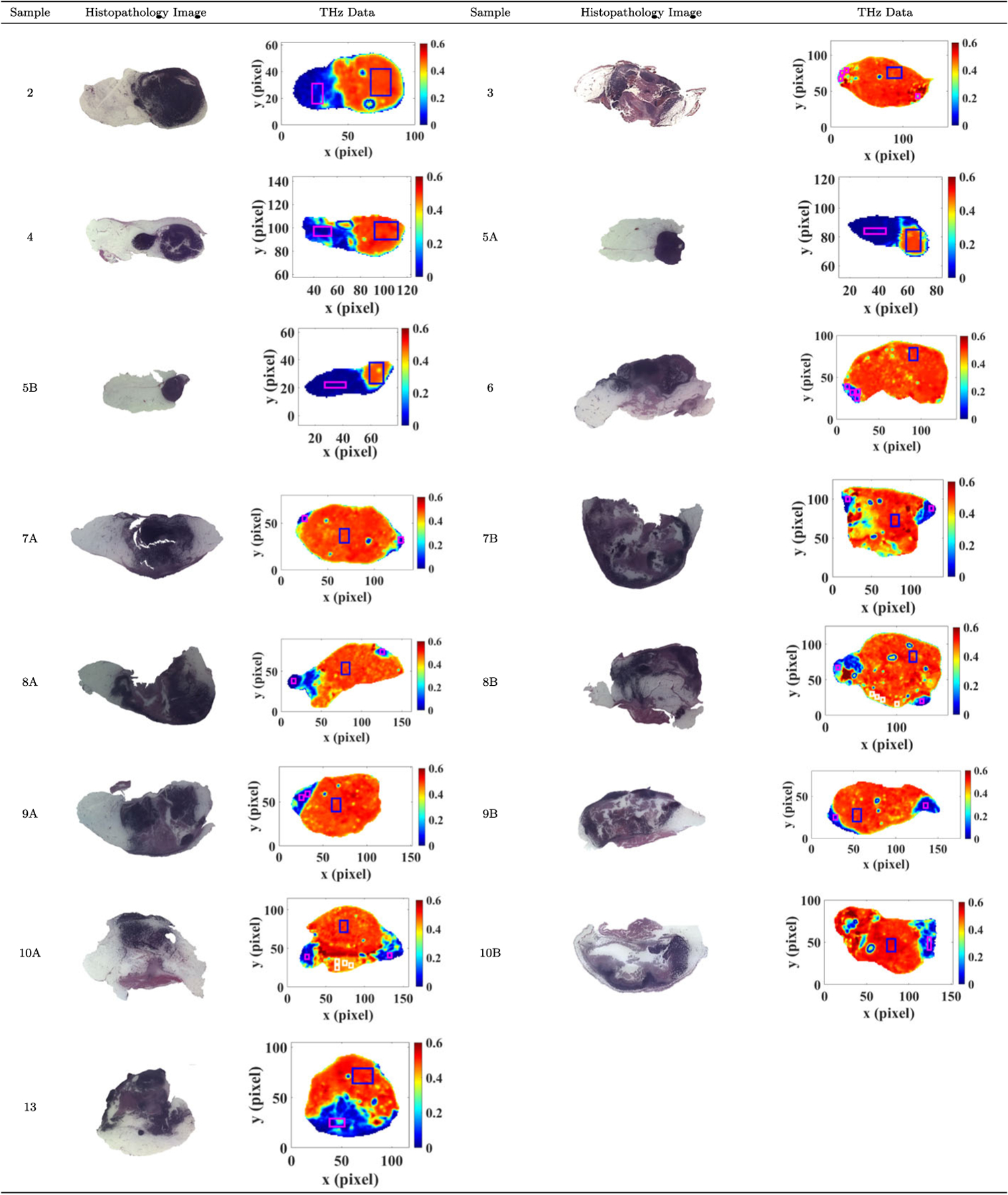
All THz images were produced in the Terahertz Imaging and Spectroscopy Lab in the Electrical Engineering Department while Pathology images were produced in the Histopathology Lab in the Biomedical Engineering Department at the University of Arkansas, Fayetteville
Footnotes
Ethics Approval All animals received care and are handled according to the guidelines in the Guide for the Care and Use of Laboratory Animals. The procedures were approved by the University of Arkansas Institutional Animal Care and Use Committee.
Consent for Publication The authors consent to publish the work upon acceptance and asked to transfer copyright of the article to the Publisher.
Conflict of Interest The authors declare no competing interests.
Code, Data, Material Availability
Code may be available upon request. Data and/or materials are not available at this time, due to institutional requirements.
References
- 1.National Breast Cancer Foundation (2020). URL https://www.nationalbreastcancer.org/breast-cancer-facts.
- 2.Lombardi A, Pastore E, Maggi S, Stanzani G, Vitale V, Romano C, Bersigotti L, Vecchione A, Amanti C, Breast Cancer: Targets and Therapy 11, 243 (2019). [DOI] [PMC free article] [PubMed] [Google Scholar]
- 3.Bowman T, Chavez T, Khan K, Wu J, Chakraborty A, Rajaram N, Bailey K, El-Shenawee MO, Journal of biomedical optics 23(2), 026004 (2018). [DOI] [PMC free article] [PubMed] [Google Scholar]
- 4.Cao Y, Chen J, Huang P, Ge W, Hou D, Zhang G, Spectrochimica Acta Part A: Molecular and Biomolecular Spectroscopy 211, 356 (2019). [DOI] [PubMed] [Google Scholar]
- 5.Eadie LH, Reid CB, Fitzgerald AJ, Wallace VP, Expert Systems with Applications 40(6), 2043 (2013). [Google Scholar]
- 6.Zhang P, Zhong S, Zhang J, Ding J, Liu Z, Huang Y, Zhou N, Nsengiyumva W, Zhang T, Current Optics and Photonics 4(1), 31 (2020). [Google Scholar]
- 7.Yamaguchi S, Fukushi Y, Kubota O, Itsuji T, Ouchi T, Yamamoto S, Scientific reports 6(1), 1 (2016). [DOI] [PMC free article] [PubMed] [Google Scholar]
- 8.Duan F, Wang YY, Xu DG, Shi J, Chen LY, Cui L, Bai YH, Xu Y, Yuan J, Chang C, World journal of gastrointestinal oncology 11(2), 153 (2019). [DOI] [PMC free article] [PubMed] [Google Scholar]
- 9.Ribeiro M, Lazzaretti AE, Lopes HS, Pattern Recognition Letters 105, 13 (2018). [Google Scholar]
- 10.Young T, Hazarika D, Poria S, Cambria E, ieee Computational intelligenCe magazine 13(3), 55 (2018). [DOI] [PMC free article] [PubMed] [Google Scholar]
- 11.Bromley J, Guyon I, LeCun Y, Säckinger E, Shah R, Advances in neural information processing systems pp. 737–737 (1994). [Google Scholar]
- 12.Araújo T, Aresta G, Castro E, Rouco J, Aguiar P, Eloy C, Polónia A, Campilho A, PloS one 12(6), e0177544 (2017). [DOI] [PMC free article] [PubMed] [Google Scholar]
- 13.Fitzgerald AJ, Wallace VP, Pinder SE, Purushotham AD, O’Kelly P, Ashworth PC, Journal of biomedical optics 17(1), 016005 (2012). [DOI] [PubMed] [Google Scholar]
- 14.Brun MA, Formanek F, Yasuda A, Sekine M, Ando N, Eishii Y, Physics in Medicine & Biology 55(16), 4615 (2010). [DOI] [PubMed] [Google Scholar]
- 15.Nakajima S, Hoshina H, Yamashita M, Otani C, Miyoshi N, Applied Physics Letters 90(4), 041102 (2007). [Google Scholar]
- 16.The Jackson Laboratory URL https://www.jax.org/about-us/why-mice.
- 17.Daubechies I, Lu J, Wu HT, Applied and computational harmonic analysis 30(2), 243 (2011). [DOI] [PMC free article] [PubMed] [Google Scholar]
- 18.Huang J, Chen B, Yao B, He W, IEEE Access 7, 92871 (2019). [Google Scholar]
- 19.Xu C, Guan J, Bao M, Lu J, Ye W, Optical Engineering 57(1), 016103 (2018). [Google Scholar]
- 20.Chavez T, Bowman T, Wu J, Bailey K, El-Shenawee M, Journal of Infrared, Millimeter, and Terahertz Waves 39(12), 1283 (2018). [DOI] [PMC free article] [PubMed] [Google Scholar]
- 21.Cheng HD, Cai X, Chen X, Hu L, Lou X, Pattern recognition 36(12), 2967 (2003). [Google Scholar]
- 22.Berg WA, Blume JD, Cormack JB, Mendelson EB, Lehrer D, Böhm-Vélez M, Pisano ED, Jong RA, Evans WP, Morton MJ, et al. , Jama 299(18), 2151 (2008). [DOI] [PMC free article] [PubMed] [Google Scholar]
- 23.Breast cancer early detection and diagnosis (2020). URL https://www.cancer.org/cancer/breast-cancer/screening-tests-and-early-detection/finding-breast-cancer-during-pregnancy.html.
- 24.Radhakrishna S, Agarwal S, Parikh PM, Kaur K, Panwar S, Sharma S, Dey A, Saxena K, Chandra M, Sud S, South Asian journal of cancer 7(2), 69 (2018). [DOI] [PMC free article] [PubMed] [Google Scholar]
- 25.Morrow M, Waters J, Morris E, The Lancet 378(9805), 1804 (2011). [DOI] [PubMed] [Google Scholar]
- 26.Nakahara H, Namba K, Wakamatsu H, Watanabe R, Furusawa H, Shirouzu M, Matsu T, Tanaka C, Akiyama F, Ifuku H, et al. , Radiation medicine 20(1), 17 (2002). [PubMed] [Google Scholar]
- 27.Erickson BJ, Korfiatis P, Akkus Z, Kline TL, Radiographics 37(2), 505 (2017). [DOI] [PMC free article] [PubMed] [Google Scholar]
- 28.Chen LC, Zhu Y, Papandreou G, Schroff F, Adam H, in Proceedings of the European conference on computer vision (ECCV) (2018), pp. 801–818. [Google Scholar]
- 29.Ronneberger O, Fischer P, Brox T, in International Conference on Medical image computing and computer-assisted intervention (Springer, 2015), pp. 234–241. [Google Scholar]
- 30.Badrinarayanan V, Kendall A, Cipolla R, IEEE transactions on pattern analysis and machine intelligence 39(12), 2481 (2017). [DOI] [PubMed] [Google Scholar]
- 31.Krizhevsky A, Sutskever I, Hinton GE, Advances in neural information processing systems 25, 1097 (2012). [Google Scholar]
- 32.Razzak MI, Naz S, Zaib A, Classification in BioApps pp. 323–350 (2018). [Google Scholar]
- 33.Rifai S, Vincent P, Muller X, Glorot X, Bengio Y, in Icml (2011).
- 34.Bochkovskiy A, Wang CY, Liao HYM, arXiv preprint arXiv:2004.10934 (2020).
- 35.Szegedy C, Liu W, Jia Y, Sermanet P, Reed S, Anguelov D, Erhan D, Vanhoucke V, Rabinovich A, in Proceedings of the IEEE conference on computer vision and pattern recognition (2015), pp. 1–9. [Google Scholar]
- 36.He K, Zhang X, Ren S, Sun J, in Proceedings of the IEEE conference on computer vision and pattern recognition (2016), pp. 770–778. [Google Scholar]
- 37.Szegedy C, Ioffe S, Vanhoucke V, Alemi A, in Proceedings of the AAAI Conference on Artificial Intelligence, vol. 31 (2017), vol. 31. [Google Scholar]
- 38.LeCun Y, Boser B, Denker JS, Henderson D, Howard RE, Hubbard W, Jackel LD, Neural computation 1(4), 541 (1989). [Google Scholar]
- 39.Huang G, Liu S, Van der Maaten L, Weinberger KQ, in Proceedings of the IEEE conference on computer vision and pattern recognition (2018), pp. 2752–2761. [Google Scholar]
- 40.Simonyan K, Zisserman A, arXiv preprint arXiv:1409.1556 (2014).
- 41.Bengio Y, Simard P, Frasconi P, IEEE transactions on neural networks 5(2), 157 (1994). [DOI] [PubMed] [Google Scholar]
- 42.Uzunova H, Schultz S, Handels H, Ehrhardt J, International journal of computer assisted radiology and surgery 14(3), 451 (2019). [DOI] [PubMed] [Google Scholar]
- 43.Baur C, Denner S, Wiestler B, Navab N, Albarqouni S, Medical Image Analysis p. 101952 (2021). [DOI] [PubMed] [Google Scholar]
- 44.Shuvo SB, Ali SN, Swapnil SI, Hasan T, Bhuiyan MIH, IEEE Journal of Biomedical and Health Informatics (2020). [DOI] [PubMed]
- 45.Roweis S, Advances in neural information processing systems pp. 626–632 (1998). [Google Scholar]
- 46.Li MD, Chang K, Bearce B, Chang CY, Huang AJ, Campbell JP, Brown JM, Singh P, Hoebel KV, Erdoğmus D¸, et al. , NPJ digital medicine 3(1), 1 (2020). [DOI] [PMC free article] [PubMed] [Google Scholar]
- 47.Chung YA, Weng WH, arXiv preprint arXiv:1711.08490 (2017).
- 48.Liu CF, Padhy S, Ramachandran S, Wang VX, Efimov A, Bernal A, Shi L, Vaillant M, Ratnanather JT, Faria AV, et al. , Magnetic resonance imaging 64, 190 (2019). [DOI] [PMC free article] [PubMed] [Google Scholar]
- 49.Mehmood A, Maqsood M, Bashir M, Shuyuan Y, Brain sciences 10(2), 84 (2020). [DOI] [PMC free article] [PubMed] [Google Scholar]
- 50.Amin-Naji M, Mahdavinataj H, Aghagolzadeh A, in 2019 4th International Conference on Pattern Recognition and Image Analysis (IPRIA) (IEEE, 2019), pp. 75–79. [Google Scholar]
- 51.Mac B, Moody AR, Khademi A, in Medical Imaging with Deep Learning (PMLR, 2020), pp. 503–514. [Google Scholar]
- 52.Hadsell R, Chopra S, LeCun Y, in 2006 IEEE Computer Society Conference on Computer Vision and Pattern Recognition (CVPR’06), vol. 2 (IEEE, 2006), vol. 2, pp. 1735–1742. [Google Scholar]
- 53.Vohra N, Bowman T, Bailey K, El-Shenawee M, Journal of visualized experiments: JoVE (158) (2020). [DOI] [PMC free article] [PubMed] [Google Scholar]
- 54.Bowman T, Vohra N, Bailey K, El-Shenawee MO, Journal of Medical Imaging 6(2), 023501 (2019). [DOI] [PMC free article] [PubMed] [Google Scholar]
- 55.Uzun IS, Amira A, Bouridane A, IEE Proceedings-Vision, Image and Signal Processing 152(3), 283 (2005). [Google Scholar]
- 56.Liu H, Zhang Y, Mantooth HA, in 2015 IEEE International Conference on Building Efficiency and Sustainable Technologies (IEEE, 2015), pp. 33–38. [Google Scholar]
- 57.Zhang Y, Liu H, Mantooth HA, in 2016 IEEE Applied Power Electronics Conference and Exposition (APEC) (IEEE, 2016), pp. 3180–3184. [Google Scholar]
- 58.Hopper G, Adhami R, Journal of the Franklin Institute 329(3), 555 (1992). [Google Scholar]
- 59.Allen J, in ICASSP ‘82. IEEE International Conference on Acoustics, Speech, and Signal Processing, vol. 7 (1982), vol. 7, pp. 1012–1015. [Google Scholar]
- 60.Tary JB, Herrera RH, van der Baan M, Philosophical Transactions of the Royal Society A: Mathematical, Physical and Engineering Sciences 376(2126), 20170254 (2018). [DOI] [PMC free article] [PubMed] [Google Scholar]
- 61.Thakur G, Brevdo E, Fučkar NS, Wu HT, Signal Processing 93(5), 1079 (2013). [Google Scholar]
- 62.El-Shenawee M, Vohra N, Bowman T, Bailey K, Biomedical Spectroscopy and Imaging 8(1–2) (2019). [DOI] [PMC free article] [PubMed] [Google Scholar]
- 63.Ho Y, Wookey S, IEEE Access 8, 4806 (2019). [Google Scholar]
- 64.Verma V, Aggarwal RK, Social Network Analysis and Mining 10(43) (2020). [Google Scholar]
- 65.C. Heather D., W. Lindsay A., G. Joseph, N. Sarah J., B. Ebonee N., M. JS, P. Charles M., T. Melissa A., N. Marc, npj Breast Cancer 4(30) (2018). [Google Scholar]
- 66.Pool R, Fat: Fighting the Obesity Epidemic, illustrated, reprint edn. (Oxford University Press, 2001). URL https://books.google.com/books?id=TF70DAAAQBAJ. [Google Scholar]
Associated Data
This section collects any data citations, data availability statements, or supplementary materials included in this article.
Data Availability Statement
Code may be available upon request. Data and/or materials are not available at this time, due to institutional requirements.