Abstract
Most pathogens are capable of infecting multiple hosts. These multiple hosts provide many avenues for the disease to emerge. In this investigation, we formulate and analyze multi-host epidemic models and determine conditions under which the disease can emerge. In particular, SIS and SIR epidemic models are formulated for a pathogen that can infect n different hosts. The basic reproduction number is computed and shown to increase with n, the number of hosts that can be infected. Therefore, the possibility of disease emergence increases with the number of hosts infected. The SIS model for two hosts is studied in detail. Necessary and sufficient conditions are derived for the global stability of an endemic equilibrium. Numerical examples illustrate the dynamics of the two- and three-host epidemic models. The models have applications to hantavirus in rodents and other zoonotic diseases with multiple hosts.
Keywords: multi-host epidemic model, basic reproduction number, hantavirus
1. Introduction
Most pathogens are capable of infecting multiple hosts, and in addition, many of these pathogens can also be transmitted by multiple hosts (Woolhouse et al., 2001). According to Woolhouse et al. (2001), approximately sixty percent of human pathogens are zoonotic causing diseases such as Lyme disease, influenza, sleeping sickness, rabies, and hantavirus pulmonary syndrome. To prevent human infection from these zoonoses, it is necessary to identify the animal reservoirs (Haydon et al., 2002). One or more animal reservoirs may exist depending on the disease and the location. For example, domestic dogs and jackals (Canis adustus) in Africa may both serve as reservoirs for the rabies virus (Haydon et al., 2002; Rhodes et al., 1998). In Britain, red foxes (Vulpes vulpes) are a reservoir population for rabies in wildlife and European badgers (Meles meles) may be a secondary host (Smith, 2002). Eliminating rabies in only one of these populations may be insufficient to prevent the disease from spreading to humans.
Hantaviruses are rodent-borne zoonotic agents that cause hemorrhagic fever with renal syndrome (HFRS) in humans throughout Europe and Asia (Schmaljohn & Hjelle, 1997). In the Americas, the infection in humans is known as hantavirus pulmonary syndrome (HPS) (Schmaljohn & Hjelle, 1997). Thirty different hantaviruses are recognized throughout the world (Mills et al., 1999; Schmaljohn & Hjelle, 1997). But each virus is primarily associated with one reservoir species that is indigenous to a particular geographic region (Chu et al., 2003; Mills et al., 1999; Schmaljohn & Hjelle, 1997; Yahnke et al., 2001). Hantaviruses are transmitted to humans primarily through inhalation of aerosolized saliva and/or excreta from infected rodents (Mills et al., 1999; Schmaljohn & Hjelle, 1997). Spillover infection to other rodents has been reported (Chu et al., 2003), but it is generally thought that these other rodents cannot maintain the disease. The role played by these other species in disease emergence or persistence is not clear.
In the present study, we are interested in the role that multiple hosts play in the emergence and persistence of disease. Our models were developed with hantavirus infection in mind, where there is a primary reservoir host and other rodents are referred to as spillover species. Rodents generally prefer certain habitats (e.g., cropland, pasture, forest) and those species carrying hantavirus strains transmissible to humans are often associated with human habitations or agriculture (Mills et al., 1999; Yahnke et al., 2001). As anthropogenic influences continually change landscape patterns (e.g., clearcutting of forests for cropland and pastures), there is greater overlap in species habitats resulting in increased contacts between rodent reservoir hosts, other rodents, and humans.
In our multi-host epidemic models, we assume that each individual in a host population is classified according to their disease status, either susceptible (S), infected (I), or recovered and immune to reinfection (R). Rodents infected with hantavirus do not shed virus for their entire life. Therefore, we study two different types of models. In the first model, infected rodents recover but do not develop immunity (SIS), and in the second model, infected rodents recover and develop immunity (SIR).
Allen and Cormier (1996) studied SIS epidemic models, similar to ours, but they considered only two hosts with no disease-related deaths. Holt and Pickering (1985) studied a two-host SIS epidemic model with exponential growth. Begon et al. (1992) included self regulation in the two-host model and free-living infective stages (Begon and Bowers, 1994). Equilibria and local stability analyses were performed for these latter models. Gandon (2004) applied multi-host SIS models to the study of parasite evolutionary dynamics. An SIS epidemic model with multiple groups within a single population was applied to gonorrhea by Lajmanovich and Yorke (1976). In this latter model, the total population size was constant and there were no births nor deaths. This model and others with multiple groups were studied by Capasso (1993) using quasimonotone methods. Other two-species models with disease affecting at least one of the two species such as predator and prey or two competing species have been analyzed (e.g., Chattopadhyay & Arino, 1999; Hadeler & Freedman, 1999; Han & Hethcote, 2001; Hethcote et al., 2004; Venturino, 1994; Venturino, 1995; 2001; 2002). In our multi-host epidemic models, species do not have a predator-prey or competitive relationship. They are related only through infection by a common pathogen. Previous models developed for hantavirus infection in rodents have been restricted to one host (Abramson & Kenkre, 2002; Abramson et al., 2003; Allen et al., 2003; 2006; Sauvage et al. 2003). In this investigation, we extend these models to n hosts. We assume that multiple hosts can be infected with the disease but one species is the primary reservoir host. The multi-host epidemic models are described in Sect. 2. The basic reproduction number, an important threshold parameter in epidemiology, is computed in Sect. 3. It is shown that the basic reproduction number can increase with n, the number of hosts. A special case of a two-host model is analyzed in Sect. 4. Necessary and sufficient conditions are derived for global stability of the endemic equilibrium. In the last section, some numerical examples for two and three-host models are presented.
2. Description of Models
First, we formulate a multi-host SIS epidemic model for n different hosts that can be infected by a common pathogen. Second, we formulate a multi-host SIR epidemic model. We assume that there is one reservoir species and n − 1 spillover species.
2.1 SIS Model
Let S1 and I1 denote the susceptible and infected reservoir species and Sj and Ij the susceptible and infected spillover species, j = 2, …, n. Each species may recover from the disease but immunity does not occur. Therefore, the model is known as an SIS epidemic model. We assume that the only interaction between species is via the disease. In particular, there are no competitor or predator-prey relationships among the populations. This is a reasonable assumption among rats and mice, carriers of hantavirus. Although rodents have many predators, we are not modeling the predator populations here, only the rodent populations. In our models, the maximal population size is limited by the availability of environmental resources, the size of the carrying capacity. Growth is regulated by a density-dependent death rate.
The SIS multi-host epidemic model is given by the following system of differential equations:
| (2.1) |
| (2.2) |
where the total population size for species j is Nj = Sj + Ij, j = 1,2, …, n. The initial conditions satisfy Sj(0) > 0 and Ij(0) ≥ 0 for j = 1,2, …, n. The birth rate for each host population j is given by bj, bj > 0. The parameter γj ≥ 0 is the recovery rate and αj ≥ 0 is the disease-related death rate for species j. In the case where γj = 0, i.e. there is no recovery from the disease, the SIS model becomes an SI model. The density-dependent death rate, dj(Nj), for species j depends on the total population size Nj. The transmission rate between an infected individual of species k and a susceptible individual of species j is βjk(Nk), βjk(Nk) ≥ 0.
To distinguish the dynamics of the reservoir species from the spillover species we assume a higher transmission rate from the reservoir species than from the spillover species or between members of the spillover species. That is,
| (2.3) |
In addition, we assume that the reservoir species has a longer period of infectivity than the spillover species. In particular, the recovery and disease-related death rates are smaller for the reservoir species than for the spillover species,
| (2.4) |
The transmission rate βjk may depend on the total population size Nk (of the infected species). We consider two well-known forms for βjk. In our models, the incidence rate βjk(Nk)SjIk/Nk can be either standard incidence or mass action incidence, where βjk(Nk) is either constant, βjk(Nk) ≡ λjk, or proportional to Nk, βjk(Nk) ≡ λjkNk, respectively. For animal populations, it is reasonable to assume a mass action incidence rate because as the population size increases so do the contacts, i.e., βjk(Nk) ≡ λjkNk (also referred to as density-dependent transmission). Mass action incidence has been assumed in some hantavirus models (Abramson & Kenkre, 2002; Abramson et al., 2003; Allen et al., 2006; Sauvage et al., 2003) and standard incidence in others (Allen et al., 2003).
The following assumptions are made concerning the density-dependent natural death rate dj(Nj).
dj ∈ C1[0,∞).
0 < dj(0) < bj − αj.
dj is increasing for Nj ≥ 0.
There exists Kj > 0 such that dj (Kj) = bj.
Assumptions (i)-(iv) imply that the total population has a logistic growth curve, a reasonable assumption for wildlife populations. Logistic growth has been assumed in models for hantavirus infection in rodents (Abramson & Kenkre, 2002; Abramson et al., 2003; Allen et al., 2003, 2006; Begon & Bowers, 1994; Begon et al., 1992; Sauvage et al., 2003) and in many other epidemic models where population growth is limited (e.g., Ackleh & Allen, 2003; 2005; Allen & Cormier, 1996; Gao & Hethcote, 1992; Mena-Lorca & Hethcote, 1992). The total population size for each host satisfies the following differential equation:
| (2.5) |
where ij = Ij/Nj is the proportion infected of species j for j = 1,2, …, n. In the absence of infection, limt→∞Nj(t) = Kj, where Kj is the carrying capacity for species j. It follows from assumptions (i)-(iv) that the total population size is positive and bounded. In particular,
| (2.6) |
where Lj is the unique solution satisfying d(Lj) = bj − αj. The disease-free equilibrium (DFE) for (2.1) and (2.2) is the unique solution satisfying S̄j = Kj and Īj = 0, j = 1,2, …, n, where the equilibrium point is denoted as E0 = (S̄1,Ī1, …, S̄n,Īn) = (K1,0, …, Kn, 0). The existence of a nonnegative endemic equilibrium E1 with Īk > 0 requires that Īj > 0 when βjk(Nk) > 0. In other words, persistence of the disease in one host population results in disease persistence in another host if there is transmission between the two.
2.2 SIR Model
In the SIR epidemic model, individuals develop immunity to the disease; an immune class, Rj, is added to the SIS multi-host epidemic model (2.1) and (2.2) for each host j. The SIR multi-host epidemic model is given by the following system of differential equations:
| (2.7) |
| (2.8) |
| (2.9) |
where Nj = Sj + Ij + Rj and Sj(0) > 0, Ij(0) ≥ 0 and Rj(0) ≥ 0 for j = 1,2, …, n. All parameters are interpreted as in the SIS model except for the parameter γj which represents the rate at which infected individuals recover and enter the immune class Rj. The total population size Nj satisfies the differential equation (2.5). Assumptions (i)-(iv) hold. Therefore, the total population size is bounded as in (2.6) and the unique DFE is given by S̄j = Kj and Īj = 0 = R̄j for j = 1,2, …, n.
3. Basic Reproduction Number
The basic reproduction number ℛ0 is one of the most important parameters in epidemiology. The basic reproduction number is defined as the average number of secondary infections that occur when an infected individual is introduced into a completely susceptible population (Dietz, 1975; Hethcote, 2000). If ℛ0 > 1, then the disease may emerge in one of the populations. However, if ℛ0 < 1, then the DFE is locally asymptotically stable (van den Driessche & Watmough, 2002). We compute the basic reproduction number for the SIS and SIR multi-host epidemic models based on the next generation approach (Diekmann et al., 1990; van den Driessche & Watmough, 2002). It is shown that the basic reproduction number is the same for both models.
Theorem 3.1
The basic reproduction number for the SIS multi-host epidemic model, (2.1) and (2.2), and the SIR multi-host epidemic model, (2.7), (2.8) and (2.9), is given by the spectral radius of the n ×n matrix ,
where
is the jk entry in the matrix Mn, j, k = 1,2, ..,n. In the special case of n = 2 hosts, the basic reproduction number is
| (3.1) |
Proof
We apply the method developed by Diekmann et al. (1990) and van den Driessche & Watmough (2002) to calculate the next generation matrix for the SIS model, equations (2.1) and (2.2), and the SIR model, equations (2.7), (2.8), and (2.9). Since these models have the same differential equations for the infectious state and the same DFE (where S̄j = Kj, j = 1,2, …, n and the other equilibrium values are zero), they have the same basic reproduction number.
The terms in the differential equations for the infected states, I = (I1, I2, …, In)T, are separated according to new infections and recovery or death. Then the system of differential equations for the vector I satisfies dI/dt = ℱ(I) − V (I), where ℱ(I) and V (I) are vector functions for the new infections and recovery or death, respectively. Computing the Jacobian matrix of these two functions, F = Dℱ and V = DV, and evaluating at the DFE, we obtain the following n ×n matrices:
| (3.2) |
and V = diag(γj+αj+bj). The basic reproduction number is the spectral radius of the matrix .
In the special case where there are n = 2 species,
| (3.3) |
It can be easily shown that the spectral radius of M2 satisfies (3.1).
In the case where there is no recovery, γk = 0 in equations (2.1) and (2.2), the SIS model becomes an SI model; Theorem 3.1 still holds true. That is, the basic reproduction number for the SI model is given by the formula in Theorem 3.1 with γk = 0.
The basic reproduction number for each species j, when there is no contact with other species, is defined by ℛjj, j = 1,2, …, n. It follows from assumptions (2.3) and (2.4) that the basic reproduction number for the reservoir species is greater than the basic reproduction number for the spillover species,
The expressions ℛjj simplify when either mass action or standard incidence are assumed. For mass action incidence, βjk(Kk) = λjkKk. The value of ℛjj simplifies to
Notice for mass action incidence that the species basic reproduction numbers increase at a rate proportional to their carrying capacity Kj. For standard incidence, βjk(Kk) = λjk so that
Favorable environmental conditions can lead to increased rodent densities (resulting in increased contacts λjk or increased carrying capacities Kj) which, in turn, can lead to hantavirus outbreaks. Increased densities of deer mice (Peromyscus maniculatus), the reservoir host for the hantavirus known as Sin Nombre virus, was one of the driving factors in the hantavirus outbreak in New Mexico in 1993 (Mills et al., 1999).
The next theorem shows that the presence of multiple species capable of transmitting the disease can result in an increase in the basic reproduction number for the system. The form of the next generation matrix is very important to verification of this next result.
Theorem 3.2
Assume that the SIS multi-host epidemic model, (2.1) and (2.2), and the SIR multi-host epidemic model, (2.7), (2.8) and (2.9), with n hosts have a basic reproduction number given by the spectral radius of the n × n matrix Mn, ρ(Mn), where Mn is defined in Theorem 3.1. If one spillover species is added to each of the model equations and all parameters of the original system with n hosts remain unchanged, then the new SIS and SIR multi-host epidemic models with n + 1 hosts has a spectral radius ρ(Mn+1) that satisfies
| (3.4) |
If, in addition, the transmission rate for host n satisfies
| (3.5) |
then
| (3.6) |
Proof
Augment the n × n matrix Mn with one row and one column of zeros, so that the augmented matrix is of size n + 1 × n + 1,
where 0 is a zero row vector of size n. Notice that the n × n submatrix of equals Mn and equals the n + 1 × n + 1 submatrix of Mn+1,
where ρ(Mn+1) is the basic reproduction number of the SIS and SIR epidemic models with n + 1 hosts. From the assumptions in the SIS and SIR multi-host epidemic models and the next generation approach, it follows that the column and row vectors A and B of matrix Mn+1 have nonnegative entries. Hence, it follows from the theory of nonnegative matrices (6.1.12, page 225, Ortega, 1987) that
If n = 1, ρ(M1) = ℛ11.
Assumption (3.5) and the assumptions regarding the nonnegativity (or positivity) of the basic parameters imply ℛn1 > 0 and ℛ1n > 0 for n ≠ 1. Consider the 2 ×2 matrix,
It is straightforward to verify that ρ(M) > ℛ11, where the inequality is strict. Applying the preceding argument shows that ρ(Mn) ≥ ρ(M). Hence, the strict inequality (3.6) holds.
Assumption (3.5) implies that there is transmission of the disease back and forth between the reservoir species and species n + 1. The system with an additional species has a basic reproduction number that is greater than the basic reproduction number of the reservoir host. The inequality (3.4) regarding the spectral radii can be applied to more general SEIR epidemic models with multiple hosts, where the state E represents individuals in a latent or exposed class.
For SIS and SIR models, it is not always the case that the basic reproduction number increases with multiple species. If either ℛn+1, j = 0 or ℛj, n+1 = 0 for all j = 1, …, n, then the basic reproduction number does not increase, but ρ(Mn+1) = ρ(Mn). For the basic reproduction number to strictly increase with the addition of a spillover species into the system, the disease must be able to infect the spillover species and also be transmitted back to the reservoir host from this spillover species (inequality (3.5) must hold).
Because hantavirus infection in rodents is primarily associated with one reservoir species, intraspecies transmission in spillover species, βjj(Kj), j = 2, …, n, may be very low or negligible. Interspecies transmission between spillover species, βkj(Kj), j, k = 2, …, n, is probably very low also. Therefore, the only positive entries in the next generation matrix may be the entries in the first column or first row, indicating there is transmission from the reservoir species to a spillover species or from a spillover to the reservoir species, respectively. There is evidence of transmission from the reservoir species to spillover species (positive antibody titers in the spillover species). Then βj1(K1) > 0 for j = 1,2, …, n; the first column of the next generation matrix Mn has positive entries. If, in addition, for some j ≠ 1, β1j(Kj) > 0, then, according to Theorem 3.2, our model predicts that the basic reproduction number in the system with the reservoir and spillover species is greater than with the reservoir host alone. For example, if ℛ11 = ρ(M1) < 1, then the presence of spillover species in the system can increase the reproduction number to a value greater than one, ℛ0 = ρ(Mn) > 1 for n > 1.
4. Two-Host SIS Epidemic Model with Standard Incidence
Consider a special case of the general n host model, where there is only the reservoir species and one spillover species. Assume that the incidence rate is standard incidence so that βjk(Nk) = λjk is constant. An explicit expression for the basic reproduction number is given in (3.1).
The SIS multi-host epidemic model (2.1) and (2.2) for n = 2 hosts can be expressed in terms of proportions. Let the proportion of infected individuals for the two hosts be denoted as i1 = I1/N1 and i2 = I2/N2. Then the differential equations for the two-host SIS epidemic model can be expressed in terms of the proportions as follows:
| (4.1) |
| (4.2) |
Based on the assumptions (i)-(iv), Nj(t) > Lj > 0 for j = 1,2. An endemic equilibrium of (2.1) and (2.2) requires that Īj > 0 and S̄j > 0, j = 1,2. Hence, there exists an endemic equilibrium of (2.1) and (2.2) if and only if there exists an endemic equilibrium of (4.1) and (4.2) with īj = Īj/(Īj+S̄j) < 1, j = 1,2. The next result states that a unique endemic equilibrium exists to the two-host SIS epidemic model if and only if ℛ0 > 1. In addition, two conditions, equivalent to ℛ0 > 1, are given that express this inequality in terms of the species basic reproduction numbers ℛjj, j = 1,2 and that relate to condition (3.5) in Theorem 3.2.
Theorem 4.1
A unique endemic equilibrium exists for the two-host SIS epidemic model (2.1) and (2.2) with standard incidence if and only if
ℛjj > 1 for some j = 1,2 or
ℛjj ≤ 1 for j = 1,2 and (1 − ℛ11)(1 − ℛ22) < ℛ12ℛ21.
Conditions (i) and (ii) are equivalent to ℛ0 > 1, where ℛ0 is defined in (3.1) and
The second inequality in part (ii) of Theorem 4.1 relates to condition (3.5) in Theorem 3.2. If the species basic reproduction numbers are less than one, ℛjj ≤ 1, j = 1,2, and if ℛ0 > 1, then there must be transmission between the reservoir and the spillover species (inequality (3.5)) because condition (ii) implies ℛ12ℛ21> 0 which implies λ12λ21 > 0. The presence of the spillover species increases the basic reproduction number of the system to a value greater than one, ℛ11 ≤ 1 < ℛ0.
Proof
The nullclines for system (4.1) and (4.2) can be expressed as
Notice that the region D = [0,1] × [0,1] is invariant for this system, that is, if ij = 0 then dij/dt > 0, and if ij = 1, then dij/dt < 0 for j = 1,2. The nullclines always intersect at the origin. Additionally, f1 has an asymptote at i1 = 1, and f2 has an asymptote at i2 = 1. The denominators of both functions are positive in the interior of region D.
First, we show conditions (i) and (ii) imply there exists a unique endemic equilibrium. We examine three different cases for the nullclines by considering the signs of the coefficients of the functions f1 and f2.
Case (i)
Suppose λ11 > γ1 +α1 + b1 and λ22 > γ2 +α2 + b2. These two inequalities are equivalent to ℛ11 > 1 and ℛ22 > 1, respectively. In addition,
The nullclines are graphed in Figure 1. There exists a unique point of intersection in the interior of D.
Fig. 1.
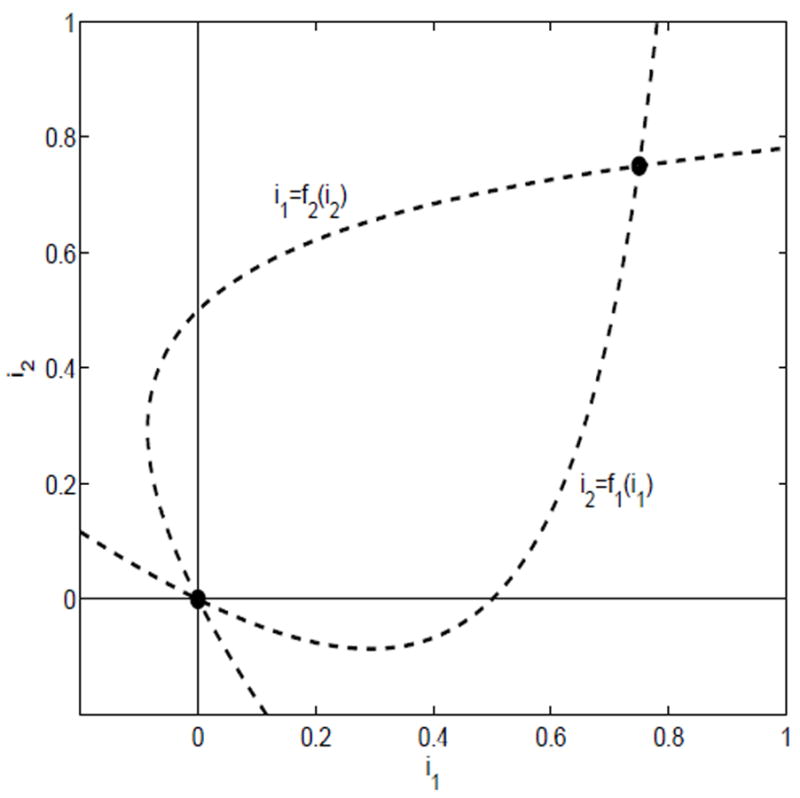
The nullclines for case (i), ℛ11 > 1 and ℛ22 > 1
Case (ii)
Suppose λ11 > γ1 + α1 + b1 and λ22 < γ2 + α2 + b2. Then ℛ11 > 1, ℛ22 < 1,
Again there exists a unique point of intersection of the nullclines in D (see Figure 2). A similar result holds if the two inequalities are reversed, when ℛ11 < 1 and ℛ22 > 1.
Fig. 2.
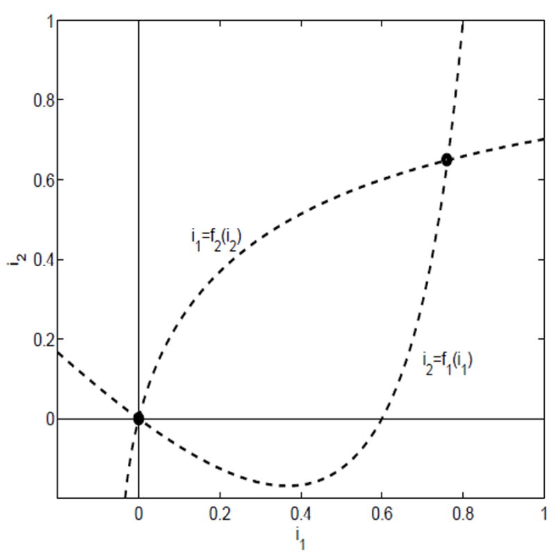
The nullclines for case (ii), ℛ11 > 1 and ℛ22 < 1
Case (iii)
Suppose λ11 < γ1 + α1 + b1 and λ22 < γ2 + α2 + b2. Then ℛ11 < 1 and ℛ22 < 1. Both nullclines have positive slope at the origin. For the nullclines to intersect in D it must be the case that the slopes at the origin satisfy
This condition can be expressed as
or equivalently (1 − ℛ11)(1 − ℛ22) < ℛ12ℛ21. Under these conditions, the nullclines cross at a unique point in the interior of the region D (see Figure 3).
Fig. 3.
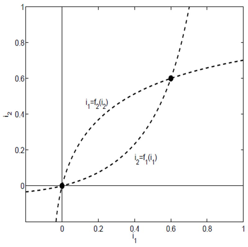
The nullclines for case (iii), ℛ11 < 1 and ℛ22 < 1 and (1 − ℛ11)(1 − ℛ22) <ℛ12ℛ21
Suppose there exists a unique endemic equilibrium but conditions (i) and (ii) are not satisfied, that is, ℛ11 < 1, ℛ22 < 1 and (1 − ℛ11)(1 − ℛ22) ≥ ℛ12ℛ21. This case cannot occur because the nullclines do not cross in the interior of the region D (see Figure 4).
Fig. 4.
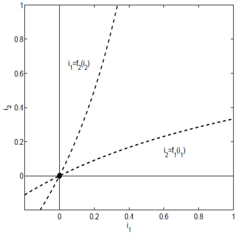
ℛ11 < 1 and ℛ22 < 1 and (1 − ℛ11)(1 − ℛ22) ≥ ℛ12ℛ21
Next we show that ℛ0 > 1 if and only if conditions (i) or (ii) hold. Suppose (i) holds. Without loss of generality, assume ℛ11 > 1 and ℛ11 > ℛ22. Then
Suppose (ii) holds. Then
Next assume ℛ0 > 1. Then
| (4.3) |
If 2 − ℛ11 − ℛ22 < 0, then either ℛ11 > 1 or ℛ22 > 1 so that condition (i) holds. If 2 − ℛ11 − ℛ22 ≥ 0, then squaring both sides of (4.3) and simplifying leads to
| (4.4) |
Thus, ℛjj ≤ 1 for j = 1,2 and inequality (4.4) implies condition (ii) holds.
Conditions similar to (i) and (ii) in Theorem 4.1 were derived by Allen and Cormier (1996). In their SIS models there was no disease-related deaths, αj = 0. Figures 1-4 illustrate the four possibilities of the nullclines and are helpful in verifying global stability of the endemic equilibrium when ℛ0 > 1.
Theorem 4.2
For the two-host SIS epidemic model (2.1) and (2.2) with n = 2 and standard incidence the basic reproduction number determines the global dynamics. In particular,
If ℛ0 ≤ 1, then the DFE is globally asymptotically stable.
If ℛ0 > 1, then the endemic equilibrium is globally asymptotically stable.
Proof
Suppose ℛ0 ≤ 1. According to Theorem 4.1, there is no endemic equilibrium. The only equilibrium is the DFE and it is locally asymptotically stable (van den Driessche & Watmough, 2002). Because solutions are bounded, Poincare-Bendixson theory can be applied. The origin is globally asymptotically stable; part (i) has been proved.
Suppose ℛ0 > 1. Then by Theorem 4.1 a unique endemic equilibrium exists. The proportions model (4.1) and (4.2) is analyzed. The endemic equilibrium for model (4.1) and (4.2) is globally asymptotically stable if and only if the endemic equilibrium for the two-host model (2.1) and (2.2) is globally asymptotically stable. The region D = [0,1] ×[0,1] is invariant for the proportions model.
First, we show that no solution can approach the DFE (the origin in the case of the proportions model). The Jacobian matrix for the proportions model evaluated at the origin is given by
The eigenvalues of J are real and are given by
where r1 = λ11 − (γ1 + α1 + b1) and r2 = λ22 − (γ2 + α2 + b2). Since ℛ0 > 1, clearly λ+ > 0. If λ− > 0, then the DFE is a repellor. If λ− < 0, the eigenvector corresponding to λ− is given by
Since λ− < 0, x2 is negative. Thus, the stable manifold of the origin lies outside the region D. No solutions approach the DFE.
Consider the i1 and i2 nullclines for system (4.1) and (4.2), i2 = f1(i1) and i1 = f2(i2), respectively (see Figures 1-4). We show that the regions enclosed by the nullclines are invariant. Along the i1-nullcline, inside the region D, but below the endemic equilibrium, di2/dt > 0 (see Figure 5). In addition, along the i2-nullcline, inside D, but to the left of the endemic equilibrium, di1/dt > 0. Thus, region A in Figure 5 is invariant. The direction of flow changes as the endemic equilibrium is crossed, so that region B is also invariant.
Fig. 5.
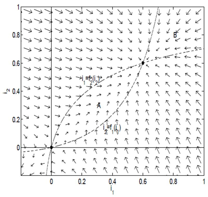
Direction field for the case ℛ11 < 1 and ℛ22 < 1 and (1 − ℛ11)(1 − ℛ22) <ℛ12ℛ21
As a result, there can be no periodic solutions inside region D. Poincare-Bendixson theory can be applied. Thus, the endemic equilibrium is globally asymptotically stable.
5. Numerical Examples
Two numerical examples are presented to illustrate the dynamics of the SIS epidemic model with standard and mass action incidence. In the first example, standard incidence is assumed, where βjk(Nk) = λjk. With only two hosts the DFE is locally asymptotically stable, ℛ0 < 1, but addition of a third host results in ℛ0 > 1. In the second example, mass action incidence is assumed, where βjk(Nk) = λjkNk. In this example, we show that increasing the carrying capacity increases the basic reproduction number and the level of prevalence.
Hantavirus in rodents results in very few, if any, disease-related deaths. Therefore, we let αj = 0.01, j = 1, …, n. We assume that conditions (2.3) and (2.4) hold. That is, λ11 > λj1 ≥ λjk, j, k = 2, …, n, λj1 ≥ λ1j, and γ1 < γj, j = 2, …, n.
In the first numerical example, for the two-host SIS epidemic model, let λ11 = 3.5, λ12 = 0.3 = λ22, λ21 = 2λ22, γ1 = 0.55, and γ2 = 1. For example, if the time period is two months, then the average length of the infectious period for the reservoir host is 1/γ1 = 3.6 months and for the spillover species it is 1/γ2 = 2 months. For the per capita birth rates, let bi = 3 for i = 1,2, where the average litter size is 6 (males and females). These are reasonable estimates based on the rice rat Oryzomys palustris which is the reservoir host for the hantavirus known as Bayou virus (Davis & Schmidley, 1994; McIntyre et al., 2005). We assume a simple form for the density-dependent death rates, d1(N1) = 0.5 + 0.005N1 and d2(N2) = 0.5 + 0.01N2. These forms result in carrying capacities of K1 = 500 and K2 = 250. The basic reproduction number for the two-host SIS epidemic model, based on these parameter values, is ℛ0 = 0.9968 < 1. Thus, the disease dies out and the DFE is globally asymptotically stable (Theorem 4.2). The dynamics over time are graphed in Figure 6 for the susceptible Sj, infected Ij, and proportion infected ij, j = 1,2. It can be seen that limt→∞ Ij(t) = 0 = limt→∞ tj(t) for j = 1,2.
Fig. 6.
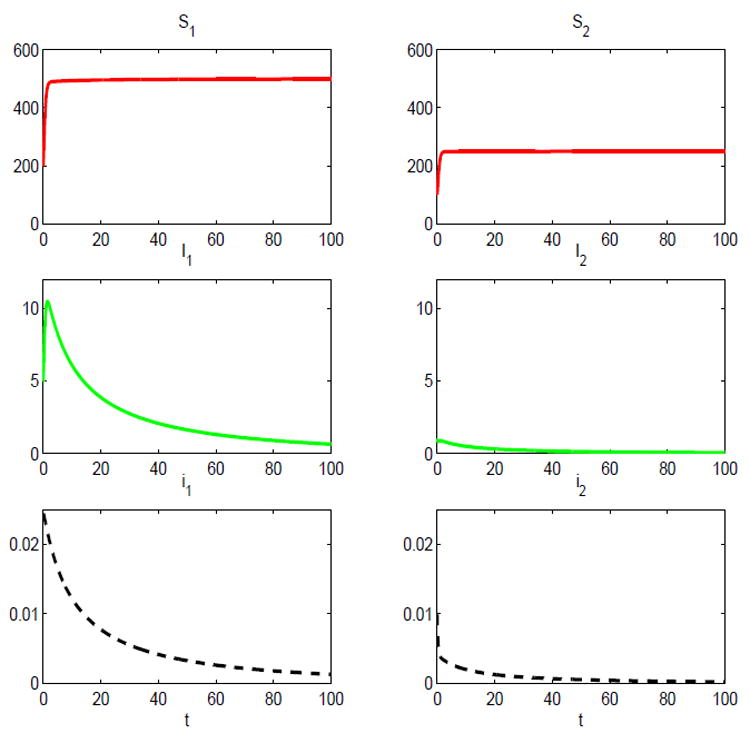
Solution of the two-host SIS epidemic model with standard incidence for initial conditions: S1(0) = 200, S2(0) = 100, I1 (0) = 5, and I2 (0) = 1; ℛ0 = 0.9968 < 1.
Suppose a third host is added to the two-host model. The third host is a spillover species similar to the second host with the same parameter values as the second host. In particular, α3 = α2, γ3 = γ2, b3 = b2, λ13 = λ33 = λ22, λ31 = λ21, d3(N3) = 0.5 + 0.01N3, and λ32 = 0 = λ23. The latter assumption implies there is no disease transmission between the two spillover species. The carrying capacity of the third species is K3 = 250. With the introduction of the third host, the basic reproduction number for the three-host SIS epidemic model increases to ℛ0 = 1.0101 > 1; the disease persists. There exists a unique endemic equilibrium which is locally asymptotically stable, (S̄1, Ī1, S̄2, Ī2, S̄3, Ī3) ≈ (495,5,249.6,0.4,249.6,0.4) (see Figure 7).
Fig. 7.
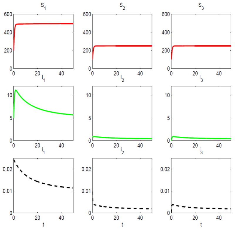
Solution of the three-host SIS epidemic model with standard incidence for initial conditions: S1(0) = 200, S2(0) = 100 = S3 (0), I1(0) = 5, I2 (0) = 1 and I3 (0) = 0; ℛ0 = 1.0101 > 1.
The prevalence of infection within the spillover species and the reservoir host is very low at the endemic equilibrium, 0.16% and 1%, respectively, but it is much greater in the reservoir host. In this example, it is the presence of the spillover species that allows the disease to persist in the system.
In the second numerical example, mass action incidence with βjk(Nk) = λjkNk is assumed. We assume the transmission rates have the same values at the carrying capacity as in the previous example, i.e., βjk(Kk) = λjk. For example, β11(K1) = 3.5 so that β11(N1) = 0.007N1. In addition, we assume β1j(Nj) = 0.0012Nj = βjj(Nj), βj1(N1) = 0.0012N1 for j = 2,3, and β23(N3) = 0 = β32(N2). With these transmission rates and the same parameter values as in the preceding three-host example, the basic reproduction number is the same, ℛ0 = 1.0101. To illustrate the impact of the carrying capacity on the dynamics, we double the carrying capacities. The same parameter values are assumed as in the preceding example, except for the density-dependent death rates and the assumptions we made regarding the transmission rates. The density-dependent death rates are d1(N1) = 0.5 + 0.0025N1, d2(N2) = 0.5 + 0.005N2, and d3(N3) = 0.5 + 0.005N3. In this second example, the carrying capacities for the three-host SIS model are K1 = 1000 and K2 = 500 = K3. When all of the carrying capacities double so does the basic reproduction number, ℛ0 = 2.0202. This can be easily seen from the next generation matrix M2 given in (3.3). The jk entry in matrix M2 is ℛjk = Kjλjk/(γk + αk + bk). An increase in Kj to 2Kj increases all of the matrix entries of M2 by a factor of 2 and as a result the spectral radius of the new matrix increases by a factor of 2.
There exists a locally stable endemic equilibrium for this three-host epidemic model given by (S̄1, Ī1, S̄2, Ī2, S̄3, Ī3) ≈ (483.7,514.3,424.8,74.9,424.8,74.9) (see Figure 8). The level of prevalence has increased substantially in this second example. At the endemic equilibrium, the total percentage of the rodent population infected is 33% (51.5% in the reservoir host and 15% in the spillover species).
Fig. 8.
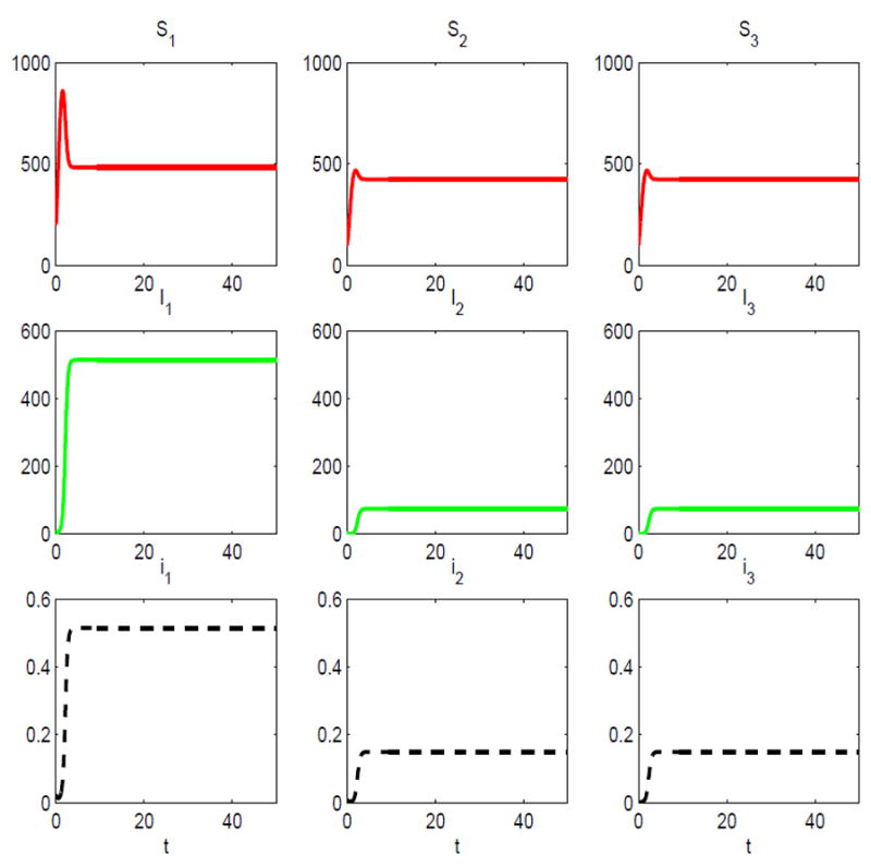
Solution of the three-host SIS epidemic model with mass action incidence for the initial conditions: S1(0) = 400, S2(0) = 200 = S3(0), I1 (0) = 5, I2(0) = 1 and I3(0) = 0; ℛ0 = 2.0202 > 1.
In a three-host SIR epidemic model with mass action incidence having the same parameter values and carrying capacities as in the second example, the basic reproduction is the same, ℛ0 = 2.0202. There is a unique locally stable endemic equilibrium in the SIR model but the prevalence of infection is less than for the SIS model (43.5% in the reservoir host and 12.4% in the spillover species).
6. Concluding Remarks
We formulated and analyzed SIS and SIR epidemic models with multiple hosts with a goal of applying our results to the study of hantavirus in rodent populations. Our analyses and simulations show that the presence of spillover species can be an important factor in the emergence and persistence of hantavirus in wild rodent populations. The important question to address for hantavirus is whether the spillover species can transmit the disease back to the reservoir host. Our theoretical results can be applied to any diseases that involve multiple hosts. The results in Theorem 3.2 imply as the number of hosts increases so does the basic reproduction number. Multiple hosts can play an important role in disease outbreaks and in disease persistence.
Acknowledgments
This research was supported by a grant from the Fogarty International Center # R01TW006986-02 under the NIH NSF Ecology of Infectious Diseases initiative. We thank the referee for helpful suggestions.
References
- Abramson G, Kenkre VM. Spatiotemporal patterns in hantavirus infection. Physical Review E. 2002;66(011912):1–5. doi: 10.1103/PhysRevE.66.011912. [DOI] [PubMed] [Google Scholar]
- Abramson G, Kenkre VM, Yates TL, Parmenter RR. Traveling waves of infection in the hantavirus epidemics. Bull Math Biol. 2003;65:519–534. doi: 10.1016/S0092-8240(03)00013-2. [DOI] [PubMed] [Google Scholar]
- Ackleh AS, Allen LJS. Competitive exclusion and coexistence for pathogens in an epidemic model with variable population size. J Math Biol. 2003;47:153–168. doi: 10.1007/s00285-003-0207-9. [DOI] [PubMed] [Google Scholar]
- Ackleh AS, Allen LJS. Competitive exclusion in SIS and SIR epidemic models with total cross immunity and density-dependent host mortality. Discrete and Cont Dyn Sys–B. 2005;5:175–188. [Google Scholar]
- Allen LJS, Cormier PJ. Environmentally-driven epizootics. Math Biosci. 1996;131:51–80. doi: 10.1016/0025-5564(95)00011-9. [DOI] [PubMed] [Google Scholar]
- Allen LJS, Langlais M, Phillips C. The dynamics of two viral infections in a single host population with applications to hantavirus. Math Biosci. 2003;186:191–217. doi: 10.1016/j.mbs.2003.08.002. [DOI] [PubMed] [Google Scholar]
- Allen LJS, McCormack RK, Jonsson CB. Mathematical models for hantavirus infection in rodents. Bull Math Biol. 2006;68:511–524. doi: 10.1007/s11538-005-9034-4. [DOI] [PMC free article] [PubMed] [Google Scholar]
- Begon M, Bowers RG. Host-host-pathogen models and microbial pest control: the effect of host self regulation. J Theor Biol. 1994;169:275–287. doi: 10.1006/jtbi.1994.1148. [DOI] [PubMed] [Google Scholar]
- Begon M, Bowers RG, Kadianakis N, Hodgkinson DE. Disease and community structure: the importance of host-self regulation in a host-pathogen model. Am Nat. 1992;139:1131–1150. [Google Scholar]
- Capasso V. Mathematical Structures of Epidemic Systems. Berlin, Heidelberg, New York: Springer-Verlag; 1993. [Google Scholar]
- Chattopadhyay J, Arino O. A predator-prey model with disease in the prey. Nonlinear Anal. 1999;36:747–766. [Google Scholar]
- Chu Y-K, Owen RD, Gonzalez L, Jonsson CB. The complex ecology of hantavirus in Paraguay. Amer J Trop Med Hyg. 2003;69:263–268. [PubMed] [Google Scholar]
- Davis B, Schmidley DJ. The Mammals of Texas. Austin, TX: Texas Parks and Wildlife Press; 1994. [Google Scholar]
- Diekmann O, Heesterbeek JAP, Metz JAJ. On the definition and the computation of the basic reproduction ratio R0 in models for infectious diseases in heterogeneous populations. J Math Biol. 1990;28:365–382. doi: 10.1007/BF00178324. [DOI] [PubMed] [Google Scholar]
- Dietz K. Transmission and control of arbovirus diseases. In: Cook KL, editor. Epidemiology. Philadelphia: SIAM; 1975. pp. 104–121. [Google Scholar]
- Gao LQ, Hethcote HW. Disease transmission models with density-dependent demographics. J Math Biol. 1992;30:717–731. doi: 10.1007/BF00173265. [DOI] [PubMed] [Google Scholar]
- Gandon S. Evolution of multihost parasites. Evolution. 2004;58:455–469. [PubMed] [Google Scholar]
- Hadeler KP, Freedman HI. Predator-prey populations with parasitic infection. J Math Biol. 1989;27:609–631. doi: 10.1007/BF00276947. [DOI] [PubMed] [Google Scholar]
- Han LZ, Ma Z, Hethcote HW. Four predator prey models with infectious diseases. Math Comp Modelling. 2001;34:849–858. [Google Scholar]
- Hethcote HW. The mathematics of infectious diseases. SIAM Review. 2000;42:599–653. [Google Scholar]
- Hethcote HW, Wang W, Han L, Ma Z. A predator-prey model with infected prey. Theor Pop Biol. 2004;66:259–268. doi: 10.1016/j.tpb.2004.06.010. [DOI] [PubMed] [Google Scholar]
- Haydon DT, Cleaveland S, Taylor LH, Laurenson MK. Identifying reservoirs of infection: a conceptual and practical challenge. Emerg Infect Dis. 2002;8:1468–1473. doi: 10.3201/eid0812.010317. [DOI] [PMC free article] [PubMed] [Google Scholar]
- Holt RD, Pickering J. Infectious disease and species coexistence: a model of Lotka-Volterra form. Am Nat. 1985;126:196–211. [Google Scholar]
- Lajmanovich A, Yorke JA. A deterministic model for gonorrhea in a nonhomogeneous population. Math Biosci. 1976;28:221–236. [Google Scholar]
- McIntyre NE, Chu YK, Owen RD, Abuzeineh A, De La Sancha N, Dick CW, Holsomback T, Nisbet RA, Jonsson C. A longitudinal study of Bayou virus, hosts, and habitat. Amer J Trop Med Hyg. 2005;73:1043–1049. [PubMed] [Google Scholar]
- Mena-Lorca J, Hethcote HW. Dynamic models of infectious diseases as regulators of population sizes. J Math Biol. 1992;30:693–716. doi: 10.1007/BF00173264. [DOI] [PubMed] [Google Scholar]
- Mills JN, Yates TL, Ksiazek TG, Peters CJ, Childs JE. Long-term studies of hantavirus reservoir populations in the southwestern United States: rationale, potential, and methods. Emerg Infect Dis. 1999;5:95–101. doi: 10.3201/eid0501.990111. [DOI] [PMC free article] [PubMed] [Google Scholar]
- Ortega JM. Matrix Theory A Second Course. New York and London: Plenum Press; 1987. [Google Scholar]
- Rhodes CJ, Atkinson RPD, Anderson RM, Macdonald DW. Rabies in Zimbabwe: reservoir dogs and the implications for disease control. Philos Trans Roy Soc Lond B Biol Sci. 1998;353:999–1010. doi: 10.1098/rstb.1998.0263. [DOI] [PMC free article] [PubMed] [Google Scholar]
- Sauvage F, Langlais M, Yoccoz NG, Pontier D. Modelling hantavirus in fluctuating populations of bank voles: the role of indirect transmission on virus persistence. J Anim Ecology. 2003;72:1–13. [Google Scholar]
- Schmaljohn C, Hjelle B. Hantaviruses: a global disease problem. Emerg Infect Dis. 1997;3:95–104. doi: 10.3201/eid0302.970202. [DOI] [PMC free article] [PubMed] [Google Scholar]
- Smith GC. The role of the Badger (Meles meles) in rabies epizootiology and the implications for Great Britain. Mammal Rev. 2002;32:12–25. [Google Scholar]
- Van den Driessche P, Watmough J. Reproduction numbers and sub-threshold endemic equilibria for compartmental models of disease transmission. Math Biosci. 2002;180:29–48. doi: 10.1016/s0025-5564(02)00108-6. [DOI] [PubMed] [Google Scholar]
- Venturino E. The influence of diseases on Lotka-Volterra systems. Rocky Mt J Math. 1994;24:381–402. [Google Scholar]
- Venturino E. Epidemics in predator-prey models: Disease in the prey. In: Arino O, Ax-elrod D, Kimmel M, Langlais M, editors. Mathematical Population Dynamics: Analysis of Heterogenity, : Theory of Epidemics. Vol. 1. Winnipeg, CA: Wuerz Pub.; 1995. pp. 381–393. [Google Scholar]
- Venturino E. The effects of diseases on competing species. Math Biosci. 2001;174:111–131. doi: 10.1016/s0025-5564(01)00081-5. [DOI] [PubMed] [Google Scholar]
- Venturino E. Epidemics in predator-prey models disease in the predators. IMA J Math Appl Med Biol. 2002;19:185–205. [PubMed] [Google Scholar]
- Woolhouse MEJ, Taylor LH, Haydon DT. Population biology of multi-host pathogens. Science. 2001;292:1109–1112. doi: 10.1126/science.1059026. [DOI] [PubMed] [Google Scholar]
- Yahnke CJ, Meserve PL, Ksiazek TG, Mills JN. Patterns of infection with Laguna Negra virus in wild populations of Calomys laucha in the central Paraguayan chaco. Am J Trop Med Hyg. 2001;65:768–776. doi: 10.4269/ajtmh.2001.65.768. [DOI] [PubMed] [Google Scholar]


