Rigorous quantification of statistical significance of the COVID-19 lockdown effect on air quality: The case from ground-based measurements in Ontario, Canada

Abstract

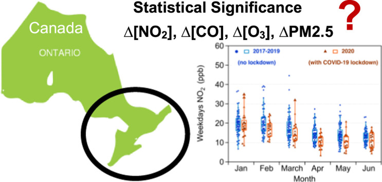
Preliminary analyses of satellite measurements from around the world showed drops in nitrogen dioxide (NO₂) coinciding with lockdowns due to the COVID-19 pandemic. Several studies found that these drops correlated with local decreases in transportation and/or industry. None of these studies, however, has rigorously quantified the statistical significance of these drops relative to natural meteorological variability and other factors that influence pollutant levels during similar time periods in previous years. Here, we develop a novel statistical protocol that accounts for seasonal variability, transboundary influences, and new factors such as COVID-19 restrictions in explaining trends in several pollutant levels at 16 ground-based measurement sites in Southern Ontario, Canada. We find statistically significant and temporary drops in NO₂ (11 out 16 sites) and CO (all 4 sites) in April-December 2020, with pollutant levels 20% lower than in the previous three years. Fewer sites (2–3 out of 16) experienced statistically significant drops in O₃ and PM2.5. The statistical significance testing framework developed here is the first of its kind applied to air quality data. It highlights the benefit of a rigorous assessment of statistical significance, should analyses of pollutant levels post COVID-19 lockdowns be used to inform policy decisions.

Graphical Abstract

1. Introduction

The province of Ontario in Canada declared a state of emergency on March 17, 2020 to limit the spread of COVID-19, which caused the first related death in mid-March 2020. As a result, lockdown restrictions affected the majority of workplaces, which shifted to working from home, , and led to the closure of recreational and shopping facilities that gather large numbers of people. Table S1 lists the timeline of restrictions in Ontario, the state of Michigan in the U.S., which borders the southwestern part of the province, and Ohio, which can influence pollution levels in Ontario via transboundary movement of pollutants. The imposition of the lockdown measures drastically reduced traffic, aviation and industrial activity in the province as reported from satellite analysis (Griffin et al., 2020). Satellite data for nitrogen dioxide (NO₂) column using the Tropospheric Monitoring Instrument (TROPOMI) operated by NASA and European Space Agency were analyzed for the Greater Toronto area, home to Ontario’s capital and Canada’s most populous urban region (Griffin et al., 2020). The analysis showed a drastic reduction in NO₂ levels by roughly 40% relative to pre-lockdown. This reduction is similar in magnitude to those reported in cities in China, Europe and the United States during their respective lockdowns and/or states of emergency (Bauwens et al., 2020). Comparisons of data in 2020 were made to the same period in 2019 to quantify the drop in NO₂ levels since weather and seasonal changes also affect the levels of these pollutants (Schiermeier, 2020). Griffin et al. (2020) estimated a 20% reduction in satellite-measured NO₂ attributed to meteorology in Toronto.

Indicator pollutants of air quality in Ontario are monitored by a network of 39 stations across the province maintained by the Ministry of the Environment, Conservation and Parks (MECP) (MECP, 2017). These pollutants include nitrogen oxides (NO_x), CO, O₃ and PM2.5. Sources of NO_x are closely associated with combustion. In 2017, 70% of NO_x originated from road vehicles and other transportation in Ontario (MECP, 2017). Seasonal variations of NO₂ levels are observed, with maximum levels occurring in the winter and minimum levels observed in the summer. The seasonal NO₂ signature can be attributed to seasonal fluctuations in the boundary layer height and variations in photochemical lifetime. In general, wind speeds increase in spring and summer as the height of the boundary layers increases, which enhances dispersion and lowers concentrations (Atkins and Lee, 1995). Also, NO₂ is a photoactive molecule that dissociates to NO and O and hence, contributes to ground-level O₃ formation. CO is a byproduct of the incomplete combustion of fossil fuels. Similar to NO_x, the transportation sector accounts for 71% of all CO emissions in Ontario (MECP, 2017). Seasonal variations of CO levels are dominated as much by photochemical lifetime as by dilution at all but the most polluted sites, with maximum levels occurring during late winter and minimum levels observed during late summer (ATSDR, 2012). This seasonal trend is the result of inversion conditions being more frequent during winter months than summer months. The major source of ground-level O₃ is secondary processes from the photochemical reaction of NO_x and volatile organic compounds (VOCs). Transportation and general solvent use account for 43% of VOCs emissions in Ontario (MECP, 2017). As a result of its formation chemistry, concentrations of ground level O₃ are highly variable on an hourly, daily, seasonally, and yearly basis. The scavenging effect of NO reduces local O₃ levels in urban centres in Ontario, especially during summer months (MECP, 2017).

Analyses of satellite and ground-based (i.e., surface) measurements of pollutant levels pre- and post-COVID-19 closures were also reported for different cities from around the globe (see references in COVID-19 and Air Pollution (2020); Casado-Aranda et al., 2021; Kroll et al., 2020; AMIGO, 2021). A 35–60% reduction in NO₂ and a 1.5–2 times increase in ground-level ozone (O₃) was reported from the hundreds of surface monitoring stations in China (Le et al., 2020, Shi and Brasseur, 2020). Also, Le et al. (2020) reported extreme levels of fine particulate matter (PM2.5) in northern China due to conditions that promoted heterogeneous aerosol chemistry. The authors did not carry out the analysis needed to account for meteorological effects on the reduction observed in NO₂ (Shi and Brasseur, 2020). For Pittsburgh, the authors reported a 50% reduction in the morning rush-hour-induced carbon monoxide (CO) and NO₂ concentrations at the high traffic sites, consistent with the 50% reduction in commuter traffic (Tanzer-Gruener et al., 2020). In this study, the authors examined weather patterns in 2020 relative to earlier years and concluded that the changes in pollutant concentrations observed in 2020 are mostly due to COVID-19 restrictions (Tanzer-Gruener et al., 2020). The analysis by Venter et al. (2020) relied on quantifying the COVID-19 lockdown effect from the difference between 2020 and predictions from a linear regression model based on historical data. Based on this analysis, the population-weighted drop in NO₂ and PM2.5 concentrations were reported to be 60% and 31%, respectively, with a 4% marginal increase in O₃ levels. However, none of the above studies has undertaken a rigorous quantification of the statistical significance associated with these findings, in that they have not quantified the extent to which the observed post-lockdown difference is merely due to the “random chance” inherently attributable to natural meteorological variation. The standard approach to establishing statistical significance is through a p-value calculation. Of the studies mentioned above, only that of Venter et al. (2020) reports p-values along with its results. However, the p-value of Venter et al. (2020) relies heavily on modeling assumptions which are difficult to verify with a small post-lockdown sample. This raises serious concerns over causality conclusions about a potential lockdown effect, particularly to the extent they inform policy decisions. This highlights the need for an in-depth analysis of the Ontario data, and the considerable challenge in accounting for short-term seasonal effects and natural variability in atmospheric chemistry when reporting an observed reduction in pollutant levels comparing pre- and post- lockdown data (Kroll et al., 2020).

This investigation aims to rigorously quantify the statistical significance of changes to air quality indicators from ground-based measurements in Southern Ontario as a result of the COVID-19 restrictions. To this end, we developed a novel statistical protocol which accounts for seasonal variability, transboundary influences, and new factors such as COVID-19 restrictions in explaining trends in the levels of NO₂, CO, O₃ and PM2.5. Importantly, key findings are supported by a statistical significance testing framework, making minimal to no modeling assumptions, being the first of its kind applied to air quality data. We expand on the relevance of this model-free framework to the analysis of a one-time event such as the lockdown in the Methods section and Supporting Information, and on implications for policy-making in the Discussion.

2. Methods

2.1. Data acquisition

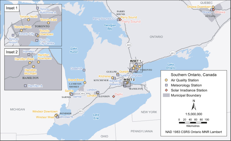
For the selected sites in this paper, ground-based hourly data of pollutant concentrations were downloaded from the MECP website (http://www.airqualityontario.com). The sites of these ambient air monitoring stations are chosen to be generally representative of regional air quality which is less influenced by immediate local sources of air contaminants. Fig. 1 shows the locations of the air quality stations, meteorology and solar irradiance stations that collect hourly data on pollutant levels, temperature and radiative forcing, respectively. These sites are classified as Rural (R) or Urban (U) by MECP, which we use here as well. This information is communicated on an hourly basis to the public through the MECP’s Air Quality Ontario website (http://www.airqualityontario.com). All instrumentation deployed at the MECP sites are US EPA designated equivalent methods. The stations, including monitoring equipment, are routinely inspected and maintained with mandatory bi-monthly onsite visits by MECP staff. The instruments are Thermo Scientific Model 42i NO-NO₂-NO_x Chemiluminescent Gas Analyzer, Thermo Scientific Model 49i O₃ analyzer, Thermo Scientific TE48C/I for CO, and Thermo Scientific Model 5030 SHARP for real-time and continuous PM-10/PM-2.5 measurement. More information regarding quality assurance and quality control can be found in reference (MECP, 2017).

Fig. 1.

Map of Southern Ontario showing locations of air quality stations maintained by MECP, national meteorological and irradiance stations maintained by ECCC.

Air quality data for all reporting years were obtained from the Air Quality Ontario website. It is important to distinguish that preliminary data are not verified while finalized data have undergone extensive quality assurance/quality control (QA/QC) procedures as outlined in the appendix of the annual Air Quality in Ontario Report (MECP, 2017). However, typically there are minimal changes applied to the dataset during the QA/QC process. A quick analysis of selected 2018 data over the time period of interest suggests that hourly and daily differences are less than 1% between preliminary and finalized data.

Hourly and daily meteorological data collected by the Meteorological Service of Canada network of stations were obtained from the National Climate Archives website (https://climate.weather.gc.ca/historical_data/search_historic_data_e.html). Solar irradiance monitoring data were obtained by contacting the surface weather observation network maintained by Environment and Climate Change Canada (ECCC).

2.2. Statistical information

The primary methodological contribution of this paper is to propose a novel approach to quantifying statistical significance for air quality data. Suppose that $N_{\mathrm{post}}$ daily pollutant concentrations are recorded post-lockdown and $N_{\mathrm{pre}}$ daily pollutant concentrations are recorded pre-lockdown under similar conditions. Specifically, in our analysis $N_{\mathrm{post}}$ corresponds to the weekdays of a given month – say April 2020 – whereas $N_{\mathrm{pre}}$ corresponds to the weekdays of the same month in the three reference years April 2017–2019. By comparing the same month across years, we accounted for natural variation in seasonal meteorology. We eliminated weekends from our analysis since we are mainly interested in the effect of COVID-19 on traffic and industrial activity, which is typically lesser on weekends.

Let Δ_obs denote the absolute difference in pre/post lockdown median pollutant levels per Eq. (1):

$${\mathrm{\Delta }}_{\mathrm{obs}}=\left|{\mathrm{Med}}_{\mathrm{pre}}-{\mathrm{Med}}_{\mathrm{post}}\right|$$ (1)

Then under the null hypothesis H ₀ that there is no difference between pre/post-lockdown data, the absolute median difference Δ_obs ought to be zero. Statistical significance formally quantifies the extent to which a non-zero value of ${\mathrm{\Delta }}_{\mathrm{obs}}$ is not merely due to random natural meteorological variations. Traditionally, statistical significance is measured by a p-value. In this case, the probability that a difference in medians obtained by repeating the data acquisition, ${\mathrm{\Delta }}_{\mathrm{rep}}$, would exceed ${\mathrm{\Delta }}_{\mathrm{obs}}$ by random chance. However, the time-dependent nature of the pollutant data renders such experimental replication inconceivable. Thus, classical p-values for these data can only be interpreted under the hypothetical construct of a statistical model, which has two related drawbacks. On the one hand, most model-based p-value calculations are only valid asymptotically. On the other hand, time-dependent data make the modeling assumptions difficult to verify - prohibitively so for the small (non-asymptotic) pre/post lockdown sample sizes $N_{\mathrm{pre}}$ and $N_{\mathrm{post}}$.

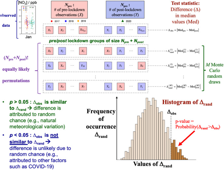
As an alternative approach, our novel statistical protocol hinges on the assessment of statistical significance via a randomization test (Fisher, 1935, Manly, 2006), which we illustrate in Fig. 2 and described below. Instead of relying on a statistical model, the randomization test takes the $N_{\mathrm{pre}}+N_{\mathrm{post}}$ observations as non-random. If there is no pre/post lockdown effect, then we may take each of the $N_{\mathrm{perm}}={(N}_{\mathrm{pre}}+N_{\mathrm{post}})!$ permutations of the observations as equally likely. The randomization p-value is calculated as shown in Eq. (2):

$$\mathrm{p}=\mathrm{Probability}\left({\mathrm{\Delta }}_{\mathrm{rand}}>{\Delta }_{\mathrm{obs}}\right)$$ (2)

where ${\Delta }_{\mathrm{rand}}$ is randomly drawn from the set of all permutations. Since it is impractical to enumerate all $N_{\mathrm{perm}}$ permutations to calculate it exactly, the randomization p-value in Eq. (2) is instead estimated to arbitrarily high precision by Monte Carlo simulation, by reporting the fraction of times ${\Delta }_{\mathrm{rand}}$ exceeds ${\Delta }_{\mathrm{obs}}$ on a large number $M\ll N_{\mathrm{perm}}$ of randomly drawn permutations (all of our p-values are calculated with $M=10000$, thus having a Monte Carlo standard error of no more than 0.005).

Fig. 2.

Graphical outline of the statistical randomization test and interpretation of the p-value.

To the best of our knowledge, this is the first application of such a randomization test to quantifying statistical significance for air quality data. Perhaps the most common randomization test is the Wilcoxon-Mann-Whitney (WMW) procedure (Mann and Whitney, 1947, Wilcoxon, 1945), which Huang et al. (2015) have used to measure spatiotemporal differences in PM2.5. WMW is a powerful test which can detect a range of departures from the null hypothesis of no lockdown effect. In contrast, our randomization test uses the difference-in-medians statistic $\mathrm{\Delta }$. This statistic focuses on a conservative overall lockdown effect that does not depend on the highest or lowest pollutant recordings, as these were found to fluctuate considerably due to natural meteorological variation. To the extent that testing $\mathrm{\Delta }$ is of specific interest, WMW is known to be invalid except under highly restrictive assumptions (Divine et al., 2018, Ludbrook and Dudley, 1998).

Classical and randomization p-values share a similar interpretation. For p > 0.05, ∆_obs is similar to ∆_rep for model-based p-values or ∆_rand for randomization p-values, hence the difference can be attributed to random chance (e.g., natural meteorological variation). If p < 0.05, ∆_obs is not similar to ∆_rep or ∆_rand, and therefore the difference is unlikely to be due to random chance (i.e., can be attributable to other factors such as COVID-19 lockdowns).

Randomization p-values have the appealing property that they are exact (up to Monte Carlo error), in that no asymptotic argument is required for their calculation. If the observations are assumed to be independent and identically distributed (iid), randomization p-values are also classical p-values which are commonly used for nonparametric significance testing (Manly, 2006). For air quality data, Zeb et al. (2019) used a different nonparametric approach to test for the presence of monotonic trends in trace gases. Unlike the randomization test proposed here, the test used by Zeb et al. is not exact in the sense that asymptotic arguments must be invoked to calculate the p-value. However, such arguments are not applicable to the small sample of measurements in each monthly comparison at hand. In the Supporting Information, a generalization of the randomization test to compare more than two reference years is proposed, and the connection between randomization and classical p-values is described in further detail.

3. Results

3.1. Assessing the trend in pollutant levels from 2008 to 2019

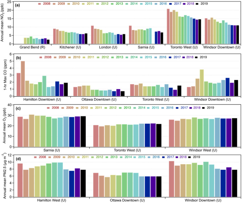
The 10-year trend in the level of pollutants that affect air quality in Ontario is shown in Fig. 3 from 2008 to 2017 per the latest air quality report from MECP (MECP, 2017). Data from 2018 and 2019 were calculated to complement the data in the report. Progressive reduction in NO_x emissions in Ontario and the US are observed because of regulations per the Clean Air Act (MECP, 2017). Fig. 3a and S1a show the annual mean trend of NO₂ for the cities in Southern Ontario analyzed in this study from 2008 to 2019 per data collected by MECP. These levels were obtained from averaging the raw hourly data and hence do not reflect seasonal effects. The 11-year trend observed in the annual mean of NO₂ appears to be leveling off for the majority of the cities in 2017–2019, which is the three-year period used here as the ‘reference’ years (see above). Levels of CO are measured in only four sites in Southern Ontario. Fig. 3b shows the 1-h maximum in CO levels at these sites. The 11-year trend in CO appears to vary by site, where there is a clear downward trend for Hamilton Downtown, Ottawa Downtown and Toronto West, and an upward trend for Windsor Downtown. The 11-year trend in O₃ levels is shown in Fig. 3c and S1b, which indicates either no change or a slight upward trend depending on the site. Similar to NO₂, these levels were obtained from averaging the raw hourly data and hence do not reflect seasonal effects. Ground level O₃ in the summer continues to exceed the Ontario Ambient Air Quality Criteria (AAQC) of 80 ppb (1-h), particularly in Southern and Eastern Ontario. As for PM2.5, the 11-year trend is shown in Fig. 3d and S1c. There is an observed downward trend overall with magnitudes varying per site. Residential sources account for 56% of all sources by sector from fuel wood combustion in fireplaces and wood stoves, followed by industrial (21%) and transportation sectors (12%) (MECP, 2017). Together, O₃ and PM2.5 drive smog episodes in May-September in Ontario, which are affected by local and regional weather patterns and long-range transboundary influences from industrial and urbanized US states. RTo To summarize, the above analysis gives a general quantification of air quality in Southern Ontario in the absence of major short-term lockdowns like the ones imposed in 2020 by the government to limit the spread of COVID-19.

Fig. 3.

Eleven-year trends in air quality pollutant levels in selected cities in Southern Ontario. The population of these cities is listed in Table 1: (a) annual mean of NO₂ levels, (b) One-hour (1-h) maximum level of CO, (c) annual mean of O₃ levels, and (d) annual mean in PM2.5 levels. Similar data for more cities are shown in Fig. S1.

3.2. Assessing variation in temperature and solar irradiance in 2017–2020

The overlap of seasonal variations in the concentrations of NO₂, CO, O₃ and PM2.5 with measures enforced by the Ontario government to limit the spread of COVID-19 complicated the assessment of reductions associated with reduced traffic, aviation, and industry emissions. To assess meteorological changes in 2020 relative to reference years, 2017–2019, Fig. S2a shows box plots of daily mean temperature for three locations selected based on their type (rural versus urban) from January until June. Similar figures were generated for the July-December period when restrictions were gradually lifted (Fig. S2b). Below each box in the plot is the p-value calculated from the randomization test described in the Methods section. The set of p-values on the right (i.e., below the 2020 data) test whether there is a statistically significant difference between the median monthly temperature in 2020 compared to 2017–2019. However, the set of p-values on the left of the box in the plot (i.e., below the 2017–2019 box data) test whether there is a statistically significant difference among the three reference years, meaning, in a given month, whether the statistical distribution of the data in 2017 is equal to that in 2018 and also to that in 2019. For March 2020, the p-value is less than 0.05 for all sites, suggesting that a potential lockdown effect on air pollutants might be masked by unusually high temperatures relative to the reference years. On the other hand, p > 0.05 for April, May, and some sites in June 2020. These data suggest that temperature was not significantly different in 2020 compared to reference years, and therefore does not confound pollutant concentrations during the months when the lockdown is both in full and waning force. The other set of p-values below the boxes to the left side tests the difference between medians in the reference years (a generalization of the randomization test above to more than two samples is provided in the Supporting Information). The p-values for February, March, and June are all greater than 0.05, indicating that 2017–2019 median temperatures were not statistically different during those months. In contrast, the corresponding p-values for January, April, and May 2017–2019 are well below 0.05. Since the months within these reference years did not experience the lockdown effect, the low p-value indicates that there is considerable natural variation in seasonal meteorology during these months, making it difficult to detect the specific impact of COVID-19 in 2020.

As shown in Fig. 1, the two stations in Southern Ontario for measuring solar irradiance are in Ottawa and Delhi. Fig. S3a shows the daily solar Global Horizontal Irradiance (GHI) at these locations from January till June between 2017 and 2020. GHI values were obtained from the measured radiation field. Similar figures were generated for the July-December period when restrictions were gradually being lifted (Fig. S3b). In this case, the p-values are generally greater than 0.05, indicating little difference in solar irradiance between these years.

3.3. Assessing variation in pollutant levels

Fig. 1 shows the locations of selected air quality stations in Southern Ontario that collect hourly data on pollutant levels analyzed here. Each air quality station measured hourly levels of NO₂, O₃ and PM2.5. Only four out of the 16 stations reported CO measurements: Hamilton Downtown, Ottawa Downtown, Toronto West, and Windsor Downtown. The MECP’s rationale behind choosing these sites for CO measurements is that Hamilton and Windsor are in the top five of the most polluted cities in Ontario. Toronto West station is near the busiest highway in North America, Hwy 401 (Dabek-Zlotorzynska et al., 2019). Ottawa was likely chosen because it is the nation’s capital city and is technically located in Eastern Ontario, further away from the US border with little industrial activity. The next few sections describe the variation in pollutant levels at different resolutions: hourly, daily, weekly and monthly in order to show how data resolution affects the type of conclusions that can be made. As detailed above, the statistical approach we developed here aims at quantifying the significance in the difference between median pollutant levels of weekdays (no weekends) per month in 2020 and the previous three years, 2017–2019, used as reference.

3.3.1. Variation in NO₂ levels

Fig. S4 shows the diurnal average levels of NO₂ in April over 2017–2019 and 2020 for Grand bend (rural), Kitchener (urban), and Toronto West (urban). These data are superimposed with solar irradiance and average hourly temperature for each location. April was chosen because it followed two weeks of COVID-19 lockdown measures in Ontario. The data show a reduction in the NO₂ levels due to photodissociation with increasing solar irradiance, which peaks around 12:00–13:00. Levels of NO₂ are also expected to decrease due to its reactions with OH/HO₂(RO₂) (Finlayson-Pitts and Pitts Jr., 2000). Overall, the average hourly concentrations of NO₂ in Grand Bend range from 1.5 to 3 ppb, Kitchener from 2.5 to 11 ppb, and from 5 to 22 ppb for Toronto West, which peak around 06:00 during the morning rush hour. While the average data in Fig. S4 show lower diurnal NO₂ levels in 2020 compared with the average data in 2017 – 2019, standard deviation calculations ( ± 1 σ) revealed extensive overlap between the two cases (see shaded areas). Based on the extensive overlap of standard deviation data, there is little evidence of a significant reduction observed in April 2020 relative to 2017–2019.

We then calculated the daily NO₂ levels for each station from January until June in 2020 for comparison with the daily average of each month from 2017 to 2019. Fig. S5-S7A show selected data for the same locations in Fig. S4. The values of the standard deviation were removed for clarity. The trends in the daily NO₂ concentrations over a five-month period show a great degree of overlap between the 2020 and average 2017 – 2019 data. Also, these data show the seasonal reduction in NO₂ in the spring months compared to winter. The start of the COVID-19 lockdown in March 2020 is marked in these Figures. There is no clear evidence that additional reductions in daily NO₂ levels were observed in the daily values in 2020 compared with the average daily values in reference years in any of the stations we analyzed. We then looked at median values of NO₂ levels for weekdays only (no weekends) for all weeks from January until the end of June, per year in 2017–2020. Figs. S5-S7B show selected data from this type of analysis for the same stations in Fig. S4. The median of weekdays analysis did not reveal clear reduction in NO₂ levels in the weeks after the COVID-19 lockdown either.

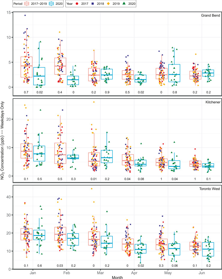
Following the hourly, daily and weekly analyses described above, the weekdays distribution in NO₂ levels in a given month in 2020 and in reference years was graphically shown using box and whisker plots. Fig. 4 shows representative plots for the three air quality stations shown in Fig. S4. The p-values for March 2020 are all statistically insignificant, perhaps linked to unusually high temperatures during this month. On the other hand, many stations recorded drops in NO₂ concentrations below the 0.05 significance level in April-June. Of particular note is Toronto West in April 2020, for which p-values below 0.05 were recorded both for 2020 relative to the reference years and between the reference years and themselves. This suggests that the drop in NO₂ in April 2020 compared to the reference years is large, even set against the considerable seasonal variability of pollutant levels which naturally occurs during the month of April. As presented in the following sections, the weekdays median values for NO₂ were used to calculate the percentage difference in 2020 relative to the reference years, 2017–2019, and to calculate the p-values used to quantify the statistical significance of the percent difference.

Fig. 4.

Box and whisker plots of NO₂ levels during weekdays (24-h average) for a given month at Grand Bend (rural), Kitchener (urban) and Toronto West (urban). Median values from these weekdays data were used to calculate percentage difference in NO₂ levels in 2020 relative to 2017–2019 as described in the text. Number below each data box corresponds to the calculated p-value. See text for details.

3.3.2. Variation in CO levels

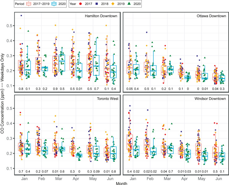
Fig. 5 shows box and whisker plots for the weekday distribution in CO levels in four air quality stations, Hamilton Downtown, Ottawa Downtown, Toronto West and Windsor Downtown. These are all urban stations, each of them having a significantly lower median CO value in April 2020 than in the reference years. There is also some evidence that the lockdown is easing, with many p-values above 0.05 in May-June 2020. Similar to NO₂, the weekdays median CO values were used to calculate the percentage difference in 2020 relative to the reference years, 2017–2019.

Fig. 5.

Box plots of CO levels during weekdays (24-h average) per month at Hamilton Downtown (urban), Ottawa Downtown (urban), Toronto West (urban) and Windsor Downtown (urban). Median values from these weekdays data were used to calculate percentage difference in CO levels in 2020 relative to 2017–2019 as described in the text. Number below each data box corresponds to the calculated p-value. See text for details.

3.3.3. Variation in O₃ and PM2.5 levels

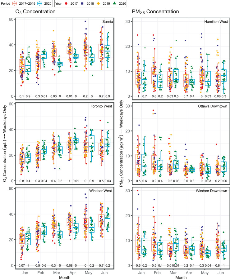
Fig. 6 shows box and whisker plots for the weekday distribution in the concentrations of O₃ and PM2.5 over 2017–2019 and 2020 for some of the sites that experienced statistically significant drops in each pollutant per Table 1. For O₃, the sites shown in the Figure are Sarnia and Windsor West, with Toronto West added for comparison given its proximity to Hwy 401. For PM2.5, the sites shown in the Figure are Hamilton West, Ottawa Downtown and Windsor Downtown. The raw data show the seasonal changes in O₃ levels for these selected sites that increase in spring and summer months. The apparent trend in PM2.5 levels is a narrower distribution of data points in May and June compared to earlier months for all years, and in 2020 in general, compared to reference years, 2017–2019. Similar to NO₂ and CO, the weekday median values for O₃ and PM2.5 were used to calculate the percentage difference in 2020 relative to the reference years, 2017–2019.

Fig. 6.

Box and whisker plots of O₃ (left panel) and PM2.5 (right panel) levels during weekdays (24-h average) per month for the sites analyzed in Fig. 4, Fig. 5. Median values from these weekdays data were used to calculate percentage difference in O₃ and PM2.5 levels in 2020 relative to 2017–2019. The number below each data box corresponds to the calculated p-value. See text for details.

Table 1.

Summary of the percentage decrease in pollutant levels in 2020 relative to the same period in 2017–2019. The statistically significant values are highlighted in p-values below 0.05 listed in parentheses.

Notes: ^a See Fig. 3 for location. ^b 2016 Census (Statistics Canada, 2016) ^c % decrease in 2020 in a given month = (median in 2020 – median in 2017–2019) * 100% / (median in 2017–2019). ‘n.o.’ = no decrease observed, on the other hand, an increase was observed in pollutant level in 2020 relative to 2017–2019.

3.4. Assessing the variability of pollutant levels within the reference years 2017–2019

Table S2 lists the p-values calculated for the concentration distribution of each pollutant within the three-year period 2017–2019 during April–June. The main assumption is that seasonal factors are the major contributors to the concentration distribution in each year, which are similar over a three-year period. The statistical significance test used here resulted in p < 0.05 for a number of sites in a given month. Tables S3-S18 list the median values for each pollutant in April–June over 2017–2019. Median values for 2020 are also listed. The median values provide an accurate indication of the similarity between years reflected in the calculations of the p-values. For example, the p-value for May in 2017–2019 for NO₂ levels at Grand Bend station is 0. The median values for NO₂ listed in Table S3 are 2.8, 4.0, and 1.6 for 2017, 2018 and 2019, respectively. Hence, the p-value of 0 indicates considerable natural variation in NO₂ concentration levels from year to year between 2017 and 2019. Other examples of statistically significant differences over the reference years are highlighted in Table S2 with underlined p-values. When the p-value for 2020 is less than 0.05, this indicates that there is a significant difference between 2020 and the past three years that could be attributed to new factors such as the COVID-19 lockdown restrictions. In the case when p-values for the reference years are also less than 0.05, this indicates that 2020 stands out despite considerable variability among the reference years. This suggests the presence of new unique factors in 2020 that are separate from those causing the difference in pollutant levels among the reference years. This result is different from the scenario where p-values are less than 0.05 for the reference years but greater than 0.05 for 2020. This result would suggest that seasonal meteorology can account for large differences between years, compared to which the lockdown effect is insignificant.

3.5. Assessing the variability of pollutant levels in 2020 relative to the reference years 2017–2019

As detailed in the Methods section, the calculated p-values reflect the degree of similarity in the distribution of daily pollutant levels in 2020 and the reference years: p-values < 0.05 indicate statistically significant difference between the 2020 median weekday levels and those in reference years. The calculated percentage difference, which could indicate increase, decrease, or no change in pollutant levels, can be attributed to new factors other than temperature and solar irradiance because it was calculated for the same monthly period. These factors would include the effect of COVID-19 measures on reducing traffic, aviation and industrial activities. It could also include new residential sources, which increased in contribution due to ‘go home and stay at home’ public health advisories starting in March 2020. Another important factor that has been known to influence air quality in Ontario is transboundary air pollution from the United States that increases the concentration of pollutants studied here. The US did not enforce COVID-19 lockdown measures during the same time period as Ontario. As highlighted in Table S1, ‘stay at home orders’ in Michigan and Ohio were implemented after Ontario and were beginning to be lifted well before Ontario lifted its ‘stay at home’ order. This difference in lockdown enforcement was expected to have a big impact on NO_x and CO levels for stations in the Windsor and Sarnia area, along the US border, which are heavily impacted by transboundary transport, in so much that any impact from COVID-19 lockdown measures would be difficult to disentangle from US sources impacting these sites.

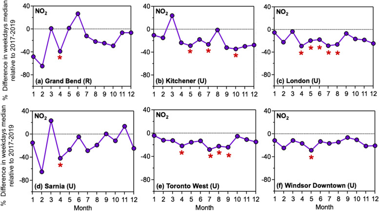
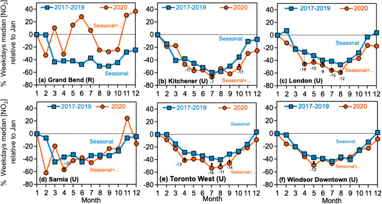
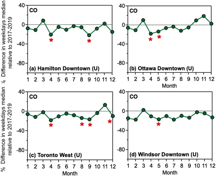
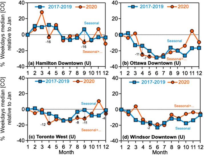
The weekday median values for the pollutants analyzed here were used to calculate the percentage difference in two ways to highlight two cases: In case 1, percentage difference values were calculated for each month in 2020 relative to the corresponding month in the reference years, 2017–2019 (Table 1). This type of calculation assumes that seasonal variability is similar for each month, and hence any statistically significant difference in pollutant levels is presumably due to new factors such as transboundary influences or COVID-19 restrictions. Fig. 7 shows graphical representation of the percentage difference in NO₂ levels for selected sites. In case 2, percentage difference values were calculated relative to January in 2020 and in the reference years 2017–2019. Then, if an extra decrease was observed for a given pollutant in 2020 relative to reference years, the difference in the percentages was calculated to quantify that extra decrease as reported in Table S19. This type of calculation shows the magnitude of seasonal changes in each pollutant for 2020 and reference years 2017–2019 relative to their highest levels in January. The assumption here was that new factors that might influence pollutant levels in 2020 beyond seasonal changes will be manifested as either increases or decreases in percentage.

Fig. 7.

Percentage difference in weekday median levels of NO₂ in 2020 relative to the same period in reference years, 2017–2019 for selected sites. The data for April–June are listed in Table 1 for these sites. The ‘*’ highlights the statistically significant decreases based on the p-values.

Fig. 8 shows graphical representation of this extra decrease in NO₂ concentrations for selected sites. Therefore, the calculated p-values were used to quantify the statistical significance of these percentages in cases 1 and 2. For Table 1 and S19, the data are only shown for April until June since COVID-19 lockdown measures started March 17, 2020 in Ontario. The statistically significant percentages are highlighted in shaded areas based on the p-values listed in parentheses. These p-values are the same as those listed in the monthly 2020 columns in Table S2. Calculated percentages that indicate no change or an increase in pollutant levels were assigned ‘n.o.’ in an effort to highlight decreases attributed to the impact of COVID-19 lockdown measures or other new factors.

Fig. 8.

Percentage difference in weekday median levels of NO₂ in 2020 and 2017–2019 relative to January of the same year(s). The vertical percentages highlight the statistically significant 'extra' decreases based on the p-values listed in Table 1 for April–June.

In order to identify the major contributors to the reduction in NO₂ observed by satellite measurements in Southern Ontario (Griffin et al., 2020), Fig. 7, Fig. 9 graphically show selected data from Table 1 for selected sites. Percentages were calculated in these Figures according to case 1 described above. Fig. 8, Fig. 10 show the extra decreases observed in 2020 for NO₂ and CO, respectively, for selected sites from percentages calculated according to case 2 described above, which are also listed in Table S19. The statistically significant decreases in NO₂ levels occurred in April and May and ranged from 18% to 42%, depending on the location of the station (Table 1). For example, Fig. 7a shows that the rural station, Grand Bend, experienced a 39% reduction in NO₂ levels in April, no change in May, and a 20% increase in June. The p-value associated with the latter percentage is 0.2 (Table S2), and hence the calculated increase in NO₂ June 2020 levels is considered statistically insignificant (i.e., June weekday median levels in 2020 are within the distribution of the corresponding values in June 2017–2019). Urban sites that experienced a statistically significant reduction in NO₂ levels in April 2020 include Guelph (22%), London (29%), Sarnia (42%), Toronto East, North, and West (~22–30%).

Fig. 9.

Percentage difference in weekday median levels of CO in 2020 relative to the same period in reference years, 2017–2019 for selected sites. The data for April–June are listed in Table 1 for these sites. The ‘*’ highlight the statistically significant decreases based on the p-values.

Fig. 10.

Percentage difference in weekday median levels of CO in 2020 and 2017–2019 relative to January of the same year(s). The vertical lines highlight the statistically significant percentage decreases based on the p-values listed in Table 1 for April–June.

Other urban sites experienced a statistically significant reduction in NO₂ levels in May 2020, which include Kitchener (29%), London (20%), Windsor Downtown and Windsor West (40%). A few urban sites experienced a reduction in NO₂ levels in June 2020, with the one in London (18%) found to be statistically significant. As shown in Fig. 7, statistically significant reductions in NO₂ were observed in some cities in July-October. During this period, gradual lifting of restrictions was taking place, with all regions of the province entering the last stage of restrictions in August (i.e., back to “normal”). However, from August to October, residents were still encouraged to limit their outings and movements (e.g., work from home when possible, limit social outings, etc.). Moreover, data in Table S19 show that the majority of sites in Southern Ontario experienced a statistically significant 4–28% extra decrease in NO₂ levels in 2020 beyond seasonal variability observed in the same months in 2017–2019. This trend in the data agrees with that shown in Table 1, with the exception of Grand Bend, where the statistically significant drop shown in Fig. 7a in April does not align with that in Fig. 8a. The box plot for the NO₂ data in Grand Bend is shown in Fig. 4 where there is a clear fluctuation in the median 2020 data over February–June relative to January compared to a progressive decrease in the corresponding data for 2017–2019. Given the location of this site on the Canadian shore of Lake Huron, it is very likely that these fluctuations are due to transboundary influences from Michigan, USA. Fig. 8 also shows the statistically significant extra reduction in NO₂ levels in 2020 for Kitchener, London and Toronto West during July-October period. Other sites that experienced similar extra reduction in NO₂ include Guelph (25%), Hamilton West (37%), Hamilton Mountain (14%), Ottawa Downtown (9%), Toronto Downtown (14–27%), and Toronto East (6–15%). As explained in the Environmental Significance section, these extra reductions might explain the lower number of day with air quality health index greater than 4 corresponding to moderate risk compared to the 2017–2019 reference years.

The data in Fig. 9 for CO levels in different urban sites show about 20% statistically significant reduction in April 2020 for Hamilton Downtown, Ottawa Downtown, and Toronto West. Windsor Downtown experienced 11% reduction in April 2020. The statistically significant reduction in CO levels continued in May 2020 for Ottawa Downtown (14%) and Windsor Downtown (17%). All of these urban sites experienced a statistically insignificant reduction in CO in June 2020, which coincided with the second phase of lifting restrictions in Ontario (see Table S1). Moreover, data in Fig. 10 show that these sites experienced a statistically significant 2–16% extra decrease in CO levels in 2020 beyond seasonal variability observed in the same months in 2017–2019. This trend in the data agrees with that shown in Fig. 9. Statistically significant extra decreases in CO were also observed for Hamilton Downtown in September (16%) and Toronto West in August and September (8% and 11%, respectively). Hamilton entered Stage 3 the third week of July, and Toronto at the end of July. So there would have been limited restrictions in August and September. This data might also reflect the influence of less ‘vacation traffic’ during this time period.

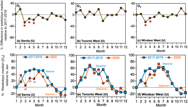
The data in Fig. 11 for O₃ levels in different urban sites show statistically significant reductions in March-May 2020 for Sarnia and Windsor West, both of which are border cities with Michigan, USA with extensive industrial activity. The reduction observed in March 2020 for these sites of nearly 40%, is greater than that observed for the Toronto West site at 24% (Fig. 11e), which is near Hwy 401. For the latter site, the reductions observed in April and May were not statistically significant. For most of the other sites, either no decreases in O₃ levels were observed in 2020, or the decreases were not statistically significant relative to the 2017–2019 reference years in the July–December period (see Tables S3-S18 for median values). These observations suggest the dominance of seasonal factors or other factors that affect the chemistry of ozone production in these sites (Kroll et al., 2020).

Fig. 11.

(a-c) Percentage difference in weekday median levels of O₃ in 2020 relative to the same period in reference years, 2017–2019. The data for April–June are listed in Table 1 for these sites. (d-f) The percentage in O₃ median values in 2020 and 2017–2019 relative to January of the same year(s). The vertical lines highlight the statistically significant percentage decreases based on the p-values listed in Table 1 for April – June.

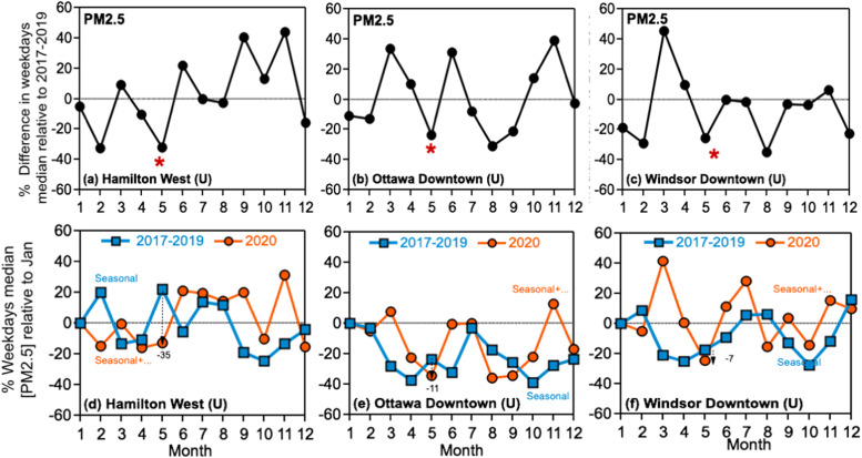
Fig. 12 a-c show the variability in PM2.5 levels for three out of four urban sites that experienced a 35–40% statistically significant reduction in May 2020, which are Hamilton West, Ottawa Downtown and Windsor Downtown. The relatively large reduction in the levels of PM2.5 in Hamilton West site was also observed when the percentage was calculated relative to January of the same year(s) (Fig. 12d). One explanation could be the effect of Ontario’s lockdown on the industrial activity in Hamilton, which was not observed in the other sites. The Ottawa Downtown site experienced 11% reduction in PM2.5 (Fig. 12e), which likely reflects the effect of the city’s lockdown on transportation. The Windsor Downtown site experienced only 7% reduction in PM2.5 (Fig. 12f), which was possibly influenced by the industrial activity in Michigan, USA. Interestingly, levels of PM2.5 were higher in June 2020 compared to previous years in all of the sites analyzed. For most of the other sites, either no decreases in PM2.5 levels were observed in 2020, or the decreases were not statistically significant relative to the 2017–2019 reference years in the July–December period (see Tables S3-S18).

Fig. 12.

(a-c) Percentage difference in weekday median levels of PM2.5 in 2020 relative to the same period in reference years, 2017–2019. The data for April–June are listed in Table 1 for these sites. (d-f) The percentage in PM2.5 median values in 2020 and 2017–2019 relative to January of the same year(s). The vertical lines highlight the statistically significant percentage decreases based on the p-values for April–June.

4. Discussion

Sites within the City of Hamilton were expected to see little impact from decreased transportation and industrial activity, as many of the city’s industry were likely classified as “essential services” during the lockdown that started in mid-March. As a result, only one site in the city had a statistically significant drop in NO₂ (Hamilton Downtown – June). The statistically insignificant drops in NO₂ at all other sites in Hamilton could be due to slowed production or could be due to annual variability driven by atmospheric chemistry (Kroll et al., 2020, Seinfeld et al., 1991). This result matches the observations of Shi and Brasseur (2020), who found substantial variability in NO₂ levels, as well as other pollutants, in Beijing, which had less severe lockdown measures than Wuhan.

In the Toronto region, NO₂ levels were expected to be significantly impacted by local sources, such as transportation and industry given their relatively large distance from significant U.S. sources of the Ohio Valley. All Toronto sites saw large drops in NO₂ levels in April 2020 relative to 2017–2019, except Toronto Downtown, which experienced 17–27% extra reduction in NO₂ during the July-October period. The drop in NO₂ levels observed here are similar to those reported by Griffin et al. (2020) after accounting for seasonality estimated in their analysis. The Toronto West site also saw a drop in measured CO levels. While not all decreases in pollutant levels were significant compared to previous years, the trend suggests that decreased movement of the population and industry played a considerable part in the observed drops. These results corroborate the findings of Griffin et al. (2020) who found that reductions in NO₂ in the Toronto region are not entirely due to COVID-19 related emissions reductions. The mix of significant and insignificant decreases from previous years could be due to the fact that a number of industries within the Toronto region were likely still operating during the lockdown, given their “essential services” status. These findings could also be highlighting the importance of other factors such as meteorology and atmospheric chemistry (Kroll et al., 2020, Seinfeld et al., 1991).

Medium sized cities in Southwestern Ontario were also expected to have little impact from transboundary sources for NO₂ with transportation making a larger impact on NO₂ and CO sources than industry. While some of these cities have manufacturing facilities, they are not expected to be on the scale of Toronto or Hamilton. As seen in Table 1, Kitchener and London had statistically significant drops in NO₂ in May and April-June, respectively. Guelph had statistically significant drops in April and during the July-October period. These data suggest that the drop in NO₂ could be directly linked with decreased traffic in these cities. This is corroborated by transportation data from Kitchener that saw a 55% decrease in traffic in early May, and a 47% decrease in late May – early June in 2020 compared to previous traffic counts within the city (Table S20). Furthermore, Ottawa experienced statistically insignificant drops in NO₂ in all three months, as well as statistically signficant drops in CO in April and May. This likely reflects the effect of the city’s lockdown on transportation and is reinforced by the findings for PM2.5 levels in the city.

Sarnia, Windsor Downtown and Windsor West were expected to have a large transboundary influence from both Michigan and Ohio, but also a potentially significant influence from transportation. Given the wide range of dates of closures and re-openings across the two US states and Ontario, it was expected that little to no difference would be seen in 2020 compared to previous years. Any difference was expected to be seen in April since all three jurisdictions were closed in this month. However, both Windsor sites saw significant decreases in NO₂ in May, with Windsor Downtown also seeing a significant decrease in CO in April and May. Sarnia saw a significant decrease of NO₂ only in April. This may suggest that Sarnia is more impacted by local transportation, including cross border traffic, as opposed to Windsor, which is impacted by local industry immediately across the border in and around Detroit. It is not clear why the Windsor sites did not see a significant drop in NO₂ April but did in May and June, which requires further analysis. Again, this finding is similar to that of Griffin et al. (2020) who found that NO₂ levels in this region of the province were difficult to recreate as a result of difficulties in estimating changes in US-based emissions due to reduced activity during COVID lockdowns.

The trends in O₃ levels where the majority of the sites did not experience statistically significant drops during April-June 2020 relative to the same period in 2017–2020 suggest that these sites are in VOC-limited region on the typical ozone isopleths such that decreasing NOx levels at low to medium VOC levels does not decrease O₃ levels (Seinfeld et al., 1991). The VOC/NOx ratio characteristic of that region is between 4:1 and 8:1 (Seinfeld et al., 1991). Quantifying the VOC/NOx ratio for different Ontario cities is currently awaiting the public availability of the 2020 VOC data for comparison with the 2017–2019 reference years.

The statistically significant drops in CO at sites across the province, especially in April, highlight the drop in transportation during the pandemic. The drop in CO concentrations continued into May, with half of the sites recording a statistically significant drop. As the province relaxed quarantine measures and the population re-emerged during May and June, the drops in CO were generally smaller than April, and not always statistically significant. For the Toronto West site, statistically significant drops in CO were also observed in August, September and December reflecting reduced traffic on Hwy401 as Ontario residents were encouraged to limit travel. This could also be a reflection of the re-implementation of restrictions in the Toronto region that began in October (see Table S1).

5. Environmental and health significance

Results presented here are highly significant because (1) quantifying the significance of short term events on pollutant levels through statistical rigor is essential for well-informed policy decisions and public confidence, (2) our analysis provides numerical evidence of the effect that large scale lockdowns have on air quality in Southern Ontario, since worsening air quality is one of the impacts of climate change (von Schneidemesser et al., 2015), and (3) policy makers would be better informed when planning for mitigation and adaptation for long-term and lasting positive effects of reducing air pollution (Ching and Kajino, 2020). For example, issuing special air quality and health advisories in Ontario relies on the calculation of the Air Quality Health Index (AQHI) directly from the 3-h average levels of NO₂, O₃ and PM2.5 (MECP, 2017) according to Eq. (3) (Stieb et al., 2008):

$$\begin{array}{c}\text{AQHI}=({\displaystyle \frac{1000}{10.4}})\times [\left({\text{e}}^{0.000537\times \text{O}3}-1\right)+\left({\text{e}}^{0.000871\times \text{NO}2}-1\right)+\hfill \\ \left({\text{e}}^{0.000487\times \text{PM}2.5}-1\right)]\hfill \end{array}$$ (3)

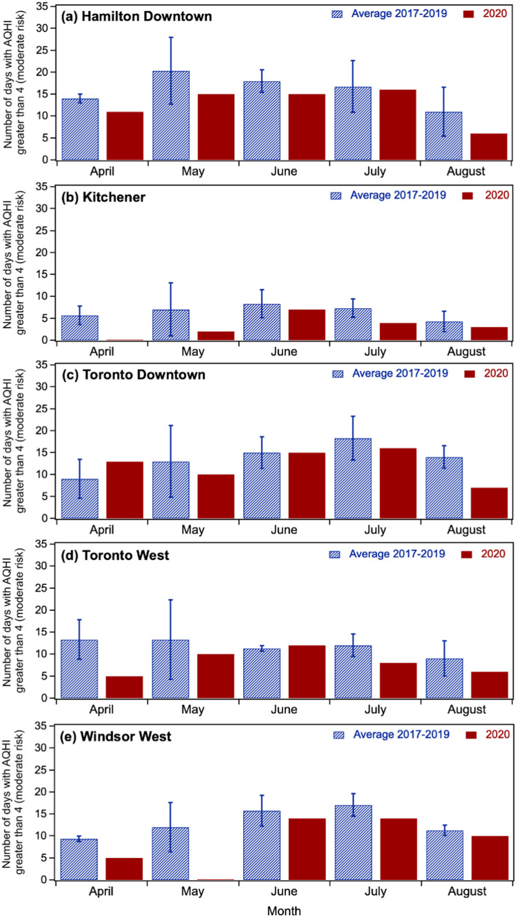
This index is used to formulate health messages to the at risk and general populations. Values of AQHI between 1 and 3 indicate ‘low risk’, 4–6 ‘moderate risk’, 7–10 ‘high risk’ and above 10 ‘very high risk’ (MECP, 2017). Fig. 13 shows, for selected cities, the average number of days when the AQHI exceeded 4 in 2017–2019 for a minimum of one time (i.e., 3 h) versus the number of days in 2020 for the spring/summer months according to the data posted on the MECP website (MECP, 2021). With the exception of Toronto Downtown which did not experience reduction in NO₂ levels in April (Table 1), there is a clear reduction in the number of days with AQHI above 4 in 2020 versus the average in the reference years 2017–2019. For Kitchener, the trend continued into May. However, within the standard deviation of the average values in 2017–2019, all the other cities showed similar number of days with AQHI above 4 for May-August. This result reflects the effect of easing COVID-19 restrictions during spring/summer months on air quality.

Fig. 13.

Comparison of the number of days with AQHI greater or equal to 4 (moderate risk, as calculated on the MECP website) in 2020 with the corresponding average for 2017–2019 reference years for selected stations during spring/summer months.

In addition, meaningful change with respect to air pollution and air quality can only be solved with meaningful local change in select circumstances. Our results highlight the impact that transboundary pollution and local industrial sources can have, limiting the effect that changing local transportation modes, as an example, can have on local air quality. Furthermore, our results also suggest that seasonal meteorology can account for large differences between years, compared to which the lockdown effect is insignificant. This highlights the importance of considering all factors that influence air pollution and that policies critical to one jurisdiction may not have a significant impact in another jurisdiction. As the province continuously monitors and reports the effect of air quality regulations for different sites, future data collection should also focus on specific chemical compounds or classes that affect local O₃ and PM2.5 formation (Kroll et al., 2020) to disentangle local versus transboundary sources.

In light of recent research that correlates long term exposure to NO₂ (Ogen, 2020), PM2.5 and PM10 in polluted cities (Zoran et al., 2020) with fatalities caused by COVID-19, future analysis should also focus on the relationship between pollution levels and the number of confirmed COVID-19 cases and deaths in the sites analyzed here. Since airborne transmission is identified as the dominant route for the spread of COVID-19 (Asadi et al., 2020, Zhang et al., 2020), research that correlates PM levels in Southern Ontario and the rates of infections and deaths are worth investigating. It is important to account for population density, age, race, socioeconomic status and establish a clear baseline from previous years on major causes of respiratory diseases and fatality.

6. Conclusions

In conclusion, the government measures to limit the spread of COVID-19 in Southern Ontario resulted in statistically significant reductions in pollutant levels emitted from the transportation and industrial sectors in the majority of the sites analyzed over April–December 2020. These reductions were beyond the seasonal variability observed within the last three years. Other sites were influenced by transboundary and/or other local influences (i.e., industry) that countered local reductions in human activity. While it is interesting to look at multiple months of data, any conclusions about the observed reductions beyond June in relating the changes directly to the impact of COVID restrictions is difficult. April and May were very much lockdown months in all jurisdictions but starting in June, as the province (and neighboring states) opened up, the potential for transport of pollutants and staggered activity across the province makes it difficult to draw clear conclusions as to why the significant decreases happened in July to December. Our paper is not attempting to say unequivocally that significant decreases in April to June are due to lockdown restrictions. However, the coincidence of reduced activity with a reduction in pollutant levels which cannot be explained by random chance strongly suggests a lockdown effect. The significant decreases beyond June, particularly at the end of the year, could be due to other factors beyond meteorological parameters, seasonal variability, and transboundary influences. This highlights the power of our statistical approach: it can find statistically significant changes in year-on-year pollutant levels even when they are not anticipated. A more in-depth analysis of transportation, commercial and industrial activity in individual municipalities during these time periods is required to make a more conclusive assessment of the pollutant changes beyond June 2020.

The city-level long- and short-term trends in pollutant levels provided herein is very useful in informing the public about the status of air quality through calculating the AQHI in response to government measures and regulations aimed at limiting the spread of new diseases or to reduce air pollution and smog episodes. Our approach also highlights the benefits of rigorous assessment of statistical significance of pollution trends in informing future policies aimed at mitigating carbon emissions in Ontario, Canada.

Author contributions

H.A conceived the idea and planned the research with the co-authors. M.L. conceived of and implemented the statistical analysis. L.N., P.P., W.M., and Y.K. collected and organized data. All authors contributed to the data analysis, discussed the results and edited the manuscript.

Declaration of Competing Interest

The authors declare that they have no known competing financial interests or personal relationships that could have appeared to influence the work reported in this paper.

Editor: Dr. H. Zaher

Appendix A. Supplementary material

Supplementary material

Data availability

The data that support the findings of this study are available from the corresponding authors upon reasonable request.

References

- AQHI in Ontario, Canada. 〈http://www.airqualityontario.com/aqhi/index.php〉.
- AMIGO (Analysis of eMissions usinG Observations), 2021. 〈https://amigo.aeronomie.be/index.php/covid-19-publications/peer-reviewed〉.
- Asadi S., Bouvier N., Wexler A.S., Ristenpart W.D. The coronavirus pandemic and aerosols: does COVID-19 transmit via expiratory particles? Aerosol Sci. Technol. 2020;54:635–638. doi: 10.1080/02786826.2020.1749229. [DOI] [PMC free article] [PubMed] [Google Scholar]
- Atkins D.H.F., Lee D.S. Spatial and temporal variation of rural nitrogen dioxide concentrations across the United Kingdom. Atmos. Environ. 1995;29:223–239. [Google Scholar]
- ATSDR . Agency for Toxic Substances and Disease Registry (ATSDR), U.S. Department of Health and Human Services Atlanta; USA: 2012. Toxicological Profile for Carbon Monoxide. [PubMed] [Google Scholar]
- Bauwens M., Compernolle S., Stavrakou T., Muller J.-F., van Gent J., Eskes H., Levelt P.F., van der A., R., Veefkind J.P., Vlietinck J., Yu H., Zehner C. Impact of coronavirus outbreak on NO2 pollution assessed using TROPOMI and OMI observations. Geophys. Res. Lett. 2020;47 doi: 10.1029/2020GL087978. e2020GL087978. https://doi.org/087910.081029/082020GL087978. [DOI] [PMC free article] [PubMed] [Google Scholar]
- Casado-Aranda L.-A., Sanchez-Fernandez J., Viedma-del-Jesus M.I. Analysis of the scientific production of the effect of COVID-19 on the environment: A bibliometric study. Environ. Res. 2021;193:1–12. doi: 10.1016/j.envres.2020.110416. [DOI] [PMC free article] [PubMed] [Google Scholar]
- Ching J., Kajino M. Rethinking air quality and climate change after COVID-19. Int. J. Environ. Res. Public Health. 2020;17(5167) doi: 10.3390/ijerph17145167. 5161-5111. [DOI] [PMC free article] [PubMed] [Google Scholar]
- COVID-19 and Air Pollution (accessed 27 August 2020). 〈https://docs.google.com/document/d/1UTQvW_OytC37IatMNR5qJK7qKfSylNpI2fT3pdteVZA/edit#heading=h.8lu90y3nmm7o〉.
- Dabek-Zlotorzynska E., Celo V., Ding L., Herod D., Jeong C.-H., Evans G., Hilker N. Characteristics and sources of PM2.5 and reactive gases near roadways in two metropolitan areas in Canada. Atmos. Environ. 2019;218(116980) 116981-116913. [Google Scholar]
- Divine G.W., Norton J.H., Barón A.E., Juarez-Colunga E. The Wilcoxon-Mann-Whitney procedure fails as a test of medians. Am. Stat. 2018;72:278–286. [Google Scholar]
- Finlayson-Pitts B.J., Pitts J.N., Jr. Academic Press; New York: 2000. Chemistry of the Upper and Lower Atmosphere. [Google Scholar]
- Fisher R.A. Oliver and Boyd; Edinburgh: 1935. The Design of Experiments. [Google Scholar]
- Griffin D., McLinden C., Racine J., Moran M., Fioletov V., Pavlovic R., Mashayekhi R., Zhao X., Eskes H. Assessing the impact of Corona-virus-19 on nitrogen dioxide levels over southern Ontario, Canada. Remote Sens. 2020;12(4112):4111–4113. [Google Scholar]
- Huang F., Li X., Wang C., Xu Q., Wang W., Luo Y., Tao L., Gao Q., Guo J., Chen S., Cao K., Liu L., Gao N., Liu X., Yang K., Yan A., Guo X. PM2.5 spatiotemporal variations and the relationship with meteorological factors during 2013-2014 in Beijing, China. PLoS One. 2015;10 doi: 10.1371/journal.pone.0141642. https://doi.org/0141610.0141371/journal.pone.0141642. [DOI] [PMC free article] [PubMed] [Google Scholar]
- Kroll J.H., Heald C.L., Cappa C.D., Farmer D.K., Fry J.L., Murphy J.G., Steiner A.L. The complex chemical effects of COVID-19 shutdowns on air quality. Nat. Chem. 2020;12:777–779. doi: 10.1038/s41557-020-0535-z. [DOI] [PubMed] [Google Scholar]
- Le T., Wang Y., Liu L., Wang J., Yung Y.L., Li G., Seinfeld J.H. Unexpected air pollution with marked emission reductions during the COVID-19 outbreak in China. Science. 2020;369:702–706. doi: 10.1126/science.abb7431. [DOI] [PMC free article] [PubMed] [Google Scholar]
- Ludbrook J., Dudley H. Why permutation tests are superior to T and F tests in biomedical research. Am. Stat. 1998;52:127–132. [Google Scholar]
- Manly B. Chapman & Hall/CRC; Boca Raton, FL: 2006. Randomization, Bootstrap and Monte Carlo Methods in Biology. [Google Scholar]
- Mann H.B., Whitney D.R. On a test of whether one of two random variables is stochastically larger than the other. Ann. Math. Stat. 1947;18:50–60. [Google Scholar]
- MECP, 2017. Air Quality in Ontario Report. 〈https://www.ontario.ca/document/air-quality-ontario-2017-report〉. Ministry of the Environment and Climate Change (currently Ministry of the Environment, Conservation and Parks (MEPC)), Toronto, ON.
- Ogen Y. Assessing nitrogen dioxide (NO2) levels as a contributing factor to coronavirus (COVID-19) fatality. Sci. Total Environ. 2020;726(138605):138601–138605. doi: 10.1016/j.scitotenv.2020.138605. [DOI] [PMC free article] [PubMed] [Google Scholar]
- Schiermeier Q. Why pollution is plummeting in some cities — but not others. Nature. 2020;580:313. doi: 10.1038/d41586-020-01049-6. [DOI] [PubMed] [Google Scholar]
- von Schneidemesser E., Monks P.S., Allan J.D., Bruhwiler L., Forster P., Fowler D., Lauer A., Morgan W.T., Paasonen P., Righi M., Sindelarova K., Sutton M.A. Chemistry and the linkages between air quality and climate change. Chem. Rev. 2015;115:3856–3897. doi: 10.1021/acs.chemrev.5b00089. [DOI] [PubMed] [Google Scholar]
- Seinfeld J.H., et al. Rethinking the Ozone Problem in Urban and Regional Air Pollution. The National Academies Press; Washington, DC: 1991. VOCs and nox: relationship to ozone and associated pollutants; pp. 163–186. [Google Scholar]
- Shi X., Brasseur G.P. The response in air quality to the reduction of chinese economic activities during the COVID‐19 Outbreak. Geophys. Res. Lett. 2020;47 doi: 10.1029/2020GL088070. e2020GL088070. https://doi.org/088010.081029/082020GL088070. [DOI] [PMC free article] [PubMed] [Google Scholar]
- Statistics Canada Population Data (2016). https://www12.statcan.gc.ca/census-recensement/2016/dp-pd/prof/index.cfm?Lang=E (Accessed August 2020).
- Stieb D.M., Burnett R.T., Smith-Doiron M., Brion O., Shin H.H., Economou V. A new multipollutant, no-threshold air quality health index based on short-term associations observed in daily time-series analyses. J. Air Waste Manag. Assoc. 2008;58:435–450. doi: 10.3155/1047-3289.58.3.435. [DOI] [PubMed] [Google Scholar]
- Tanzer-Gruener R., Li J., Eilenberg S.R., Robinson A.L., Presto A.A. Impacts of modifiable factors on ambient air pollution: a case study of COVID-19 shutdowns. Environ. Sci. Technol. Lett. 2020;7:554–559. doi: 10.1021/acs.estlett.0c00365. [DOI] [PubMed] [Google Scholar]
- Venter Z.S., Aunan K., Chowdhury S., Lelieveld J. COVID-19 lockdowns cause global air pollution declines. Proc. Natl. Acad. Sci. USA. 2020;117:18984–18990. doi: 10.1073/pnas.2006853117. [DOI] [PMC free article] [PubMed] [Google Scholar]
- Wilcoxon F. Individual comparisons by ranking methods. Biom. Bull. 1945;1:80–83. [Google Scholar]
- Zeb N., Khokhar M.F., Pozzer A., Khan S.A. Exploring the temporal trends and seasonal behaviour of tropospheric trace gases over Pakistan by exploiting satellite observations. Atmos. Environ. 2019;198:279–290. [Google Scholar]
- Zhang R., Li Y., Zhang A.L., Wang Y., Molina M.J. Identifying airborne transmission as the dominant route for the spread of COVID-19. Proc. Natl. Acad. Sci. USA. 2020;117:14857–14863. doi: 10.1073/pnas.2009637117. [DOI] [PMC free article] [PubMed] [Google Scholar]
- Zoran M.A., Savastru R.S., Savastru D.M., Tautan M.N. Assessing the relationship between surface levels of PM2.5 and PM10 particulate matter impact on COVID-19 in Milan, Italy. Sci. Total Environ. 2020;738(139825) doi: 10.1016/j.scitotenv.2020.139825. 139821-139812. [DOI] [PMC free article] [PubMed] [Google Scholar]
Associated Data
This section collects any data citations, data availability statements, or supplementary materials included in this article.
Supplementary Materials