Risky business: How an herbivore navigates spatiotemporal aspects of risk from competitors and predators

Abstract

Understanding factors that influence animal behavior is central to ecology. Basic principles of animal ecology imply that individuals should seek to maximize survival and reproduction, which means carefully weighing risk against reward. Decisions become increasingly complex and constrained, however, when risk is spatiotemporally variable. We advance a growing body of work in predator–prey behavior by evaluating novel questions where a prey species is confronted with multiple predators and a potential competitor. We tested how fine‐scale behavior of female mule deer (Odocoileus hemionus) during the reproductive season shifted depending upon spatial and temporal variation in risk from predators and a potential competitor. We expected female deer to avoid areas of high risk when movement activity of predators and a competitor were high. We used GPS data collected from 76 adult female mule deer, 35 adult female elk, 33 adult coyotes, and six adult mountain lions. Counter to our expectations, female deer exhibited selection for multiple risk factors, however, selection for risk was dampened by the exposure to risk within home ranges of female deer, producing a functional response in habitat selection. Furthermore, temporal variation in movement activity of predators and elk across the diel cycle did not result in a shift in movement activity by female deer. Instead, the average level of risk within their home range was the predominant factor modulating the response to risk by female deer. Our results counter prevailing hypotheses of how large herbivores navigate risky landscapes and emphasize the importance of accounting for the local environment when identifying effects of risk on animal behavior. Moreover, our findings highlight additional behavioral mechanisms used by large herbivores to mitigate multiple sources of predation and potential competitive interactions.

INTRODUCTION

An animal's niche is defined by the environmental, spatial, and temporal resources used (Vandermeer, 1972) and has evolved over time to include biotic and abiotic factors that determine the presence, survival, and reproduction of a population (Gaillard et al., 2010). In an ideal world, access to forage resources would be unlimited and freely available to animals. In natural settings, however, the complete suite of resources are not freely available, and selection of resources is limited by external factors such as predation, competition, and thermal environment (Long et al., 2014), among others (Kacelnik et al., 1992).

In theory, animals should make decisions that aim to maximize fitness, but optimal use of the landscape is often limited by many constraining factors (Bergman et al., 2001; Lima, 1998; Parker et al., 2009; Pyke, 1984). Intra‐ and interspecific competition are expected to promote resource partitioning and differential habitat use among species assemblages. Interference competition often results in patterns of spatial displacement or avoidance behavior by poor competitors (Johnson et al., 2000; Merems et al., 2020). Competitive interactions between elk (Cervus canadensis) and cattle (Bos taurus) resulted in spatial displacement of elk when cattle were present (Stewart et al., 2002). Similarly, the presence of elk resulted in avoidance by mule deer (Odocoileus hemionus), suggesting elk‐mediated constraints on habitat selection by mule deer and potential interference competition (Johnson et al., 2000). Competitive interactions may translate to a risk of nutritional loss for poor competitors, especially if poor competitors are displaced into lower‐quality habitat (Merems et al., 2020; Stewart et al., 2011).

Although competitive interactions have the potential to indirectly affect survival through nutritional deficits, predation risk is a direct risk to prey survival. A plethora of research has identified the importance of predation in influencing selection of resources by animals (Altendorf et al., 2001; Bergerud & Page, 2011; Brown, 1988; Creel & Winnie, 2005). Relative to the indirect forms of risk from competitive interactions, predation acts as a direct risk to survival (i.e., consumptive effects), or indirectly, through a perceived risk of predation that forces behavioral modifications of prey (i.e., non‐consumptive or risk effects). Such modifications include reductions in foraging time or increased vigilance (Bøving & Post, 1997; Brown, 1999; Creel et al., 2014; Verdolin, 2006), increased movement rate (Frair et al., 2005; Middleton et al., 2013; Proffitt et al., 2009), and shifts in habitat use to areas of lower risk of predation (Cowlishaw, 1997; Ripple & Beschta, 2004; Sinclair, 1985). Risk effects and consumptive effects of predation both have the ability to affect prey behavior, and ultimately, prey survival (Brown & Kotler, 2004; Creel et al., 2014; Creel & Winnie, 2005; Slos & Stoks, 2008).

Responses of prey to spatial variation in predation risk have been examined in detail (Altendorf et al., 2001; Creel & Winnie, 2005; Gervasi et al., 2013); however, the majority of these evaluations incorporate only a single predator species, which is problematic in multi‐predator systems where different predators invoke different antipredator responses of prey (Kohl et al., 2019). In systems where prey face multiple sources of predation, along with potential competitive interactions, the challenge of balancing risks becomes increasingly difficult. The spatial distribution of risk from predation and potential competition may create the situation where avoidance of one source of risk results in increased exposure to another source of risk (Courbin et al., 2019; Cusack et al., 2020; Kohl et al., 2018, 2019; Valeix et al., 2009).

An alternative or additional solution to shifting space use could be to alter activity patterns when activity of predators or competitors is highest or when hunting success of predators is maximized (Crawford et al., 2021; Gaynor, 2019; Kohl et al., 2018; Palmer et al., 2017; Smith et al., 2019). For instance, coursing predators who rely on visual cues are more likely to hunt during dawn and dusk, whereas ambush predators who rely on being undetected may hunt in darkness (Kohl et al., 2018, 2019; Pierce et al., 2004). Divergent activity patterns of predators may provide an opportunity for prey to exploit time periods when activity of predators is low. Alterations in prey activity and space use relative to the risk of predation has recently been demonstrated (Kohl et al., 2019; Smith et al., 2019), however, such patterns exist in heterogeneous environments (e.g., grasslands intermixed within forest patches) where cues of predation risk are easily perceived (Kohl et al., 2019; Smith et al., 2019). The question remains as to how animals navigate relatively homogeneous landscapes where cues of risk may be less predictable.

Responses to risk, whether shifts in space use or activity patterns, can vary as a function of the amount of risk experienced (e.g., functional response in habitat selection). Caribou (Rangifer tarandus) were more likely to select patches of food resources when closer to escape cover from wolves (Canis lupus), allowing caribou to spend more time foraging in safe areas (Mason & Fortin, 2017). Functional responses in animal–habitat relationships are crucial for characterizing individual heterogeneity in responses to environmental resources (Holbrook et al., 2019), and therefore are a useful tool to assess context‐dependent decisions relative to risk (Mason & Fortin, 2017). Evaluating functional responses in resource selection provides a powerful opportunity to uncover how prey navigate a gradient of multiple, competing risks across risky landscapes.

Here, we evaluated fine‐scale responses of female mule deer (hereafter, referred to as “deer”) to spatial and temporal heterogeneity in risk during a period in which females are experiencing the greatest nutritional demands (i.e., late gestation and lactation): May to September (Monteith et al., 2014; Parker et al., 2009). We tested whether resource selection by deer at the resolution of movement steps varied with spatial or temporal variation in interactions with elk (i.e., potential competitor) and the risk of encounter with coyotes (Canis latrans) and mountain lions (Puma concolor), along with the risk of predation by mountain lions (all collectively referred to as “risk” hereafter). We did not evaluate responses of deer to risk of predation by coyotes because of data limitations and there may be fewer reliable environmental cues to signal how cursorial predators capture prey (Kohl et al., 2019; Preisser et al., 2007).

We expected that deer would avoid all forms of risk along their movement path, however, avoidance of the risk of predation by mountain lions would be strongest because risk of direct mortality should promote the greatest behavioral response (Crosmary et al., 2012; Thaker et al., 2011; Valeix et al., 2009). Alternatively, deer may not be able to avoid risk within their home range, and instead selection for risk should vary according to the amount of risk they are exposed to within their home range (Figure 1c). We evaluated whether the average level of risk that a female experienced within her home range influenced the degree to which they avoided risk along their movement paths. To test whether deer avoided risky places during risky times (i.e., when activity of predators or competitors is high) we examined whether deer reduced overlap in movement activity (i.e., hourly movement rates; Ensing et al., 2014; Kohl et al., 2018, 2019; vander Vennen et al., 2016) as the amount of risk they were exposed to within their home range increased. We expected that if variation in activity of predators and a potential competitor were key for deer to avoid risk, temporal overlap in movement activity of deer with elk, coyotes, and mountain lions would decrease with increasing levels of risk within their home range (Figure 1d). Our analyses merge expectations of life‐history theory, predator–prey interactions, and movement ecology to parse out the importance of competing risks on prey behavior in a dynamic and multi‐species system.

FIGURE 1.

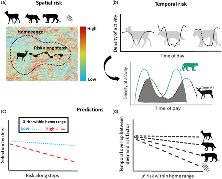
Conceptual diagram illustrating our approach to address our research questions: (1) How does space use and movement by female deer change relative to spatial and temporal variation in risk? (2) How do movement activity patterns of female deer change as spatial exposure to risk increases? We first developed metrics of the (a) spatial distribution of risk including the risk of encounter with elk, coyotes, and mountain lions, as well as the risk of predation by mountain lions, and (b) temporal variation in risk represented as overlap in movement activity (indexed by hourly movement rate [m/h]) between individual female deer, and elk, coyotes, and mountain lions. We expected that females may exhibit a functional response to risk, and selection or avoidance of risk may be modulated by (c) the average level of risk ($\overline{x}$) within their home range and (d) if females are shifting movement activity in response to risk, temporal overlap in activity between female mule deer and risk factors should decrease as the average risk within home ranges increases.

MATERIALS AND METHODS

Study area

Our study occurred in the Greater Little Mountain Ecosystem (6400 km²; 41°4′26.22″ N 109°3′1.80″ W) located in southwest Wyoming, USA during late spring and summers of 2018, and 2019. Our study area was a high‐desert system with low‐elevation (~1800 m) valleys of mixed sage‐grassland (Artemisia spp., blue‐bunch wheatgrass [Pseudoroegneria spicata], and cheatgrass [Bromus tectorum]) that transitioned into patchworks of pinyon‐juniper (Juniperus spp.) at intermediate elevations (~2400 m) and pockets of quaking aspen (Populus tremuloides) and subalpine fir (Abies lasiocarpa) at high elevations (~2700 m). Climate was characterized by long and often severe winters and short, dry summers. Snowfall during winter 2017–2018 was less severe (92% of median snowpack) than that of 2018–2019 (103% of median snowpack; NRCS Snowpack Data). Average summer precipitation from May to July in 2018 was 2.7 cm and 3.6 cm in 2019. May precipitation in 2018 was well above the average from 1981 to 2010, however, precipitation plummeted to 45% of average by July 2018, producing drought‐like conditions across the study area during that year (SNOTEL Data, Green River Station).

Our study area harbored populations of several ungulate species including elk, mule deer, pronghorn (Antilocapra americana), feral horses (Equus ferus), and Shiras moose (Alces alces shirasi), although density of feral horses and Shiras moose were relatively low. Predators in our study area included mountain lions, coyotes, and the occasional black bear (Ursus americanus). The 3‐year trend count for elk in our study area hovered between 500 and 600, and the mule deer population was estimated at 3650–4000 (Wyoming Game and Fish Department [WGFD] Job Completion Reports). Mountain lions were the primary predator of adult mule deer: 18% of mortalities of adult mule deer that occurred in 2018 and 2019 were attributed to mountain lions, and zero mortalities were attributed to coyotes. Coyotes were accountable for 14% of neonate mortalities and mountain lions contributed 24% of neonate mortalities in 2018 and 2019. Human disturbance in our study area is limited to recreational travel by passenger vehicles and all‐terrain vehicles (ATVs). Furthermore, harvest of female mule deer is prohibited, and hunting season of males does not occur until October of each year after our study period ends.

Analytical overview

Our analytical approach to addressing our hypotheses required multiple, nested analyses (Figure 1). First, we developed multiple metrics to quantify the spatial distribution of risk across the study area, including the probability of encounter with elk, coyotes, and mountain lions as well as the risk of predation by a mountain lion (Figure 1a). From the modeled distribution of risk, we calculated two metrics of use by deer. First, we extracted values of modeled risk (i.e., encounter or risk of predation) to GPS locations of female mule deer to represent risk experienced by deer along their movement path (Figure 1a). Additionally, we calculated the mean value of risk within each deer home range to represent exposure to risk within their local environment (Figure 1a). To explore whether deer minimized movement activity during peaks in elk, coyote, or mountain lion activity, we first calculated species‐specific curves of diel activity (measured as movement rate in m/h) for elk, coyotes, and mountain lions (Figure 1b). We then calculated temporal overlap in movement activity between each individual deer, and the species‐specific curve of activity for elk, coyotes, and mountain lions; we used these values to represent overlap in activity between each individual deer and elk, coyotes, and mountain lions (Figure 1b). Finally, we used the derived estimates of spatial risk (i.e., probability of encounter and predation risk within deer home ranges and along steps) to evaluate (1) how movement and space use of deer varies according to spatial distribution of risk and (2) how deer modify movement activity patterns relative to risk.

Data collection

To evaluate responses of deer to risk of encounter with elk, coyotes, and mountain lions as well as the risk of predation by mountain lions, we used GPS data from 76 female mule deer, 35 adult female elk, 33 adult coyotes (15 female, 18 male), and six adult mountain lions (4 female, 2 male). We captured mountain lions from May 2016 to April 2018 using baited cage traps and hounds. Upon capture, we anesthetized mountain lions with 1.8 mg/kg body mass of a combination of tiletamine and zolazepam hydrochloride (Telazol), and fitted them with a GPS collar (Telonics, Inc., Mesa, Arizona, USA) programmed to collect a location at 3‐h intervals before 1 May and 1‐h intervals after 1 May until 30 September. We determined sex and estimated age of each captured mountain lion via tooth replacement and wear (Gier, 1957) and waited for animals to regain conciousness (usually about 1 h) before leaving the capture location. Capture of mountain lions was performed by WGFD and permitted under WGFD Chapter 33 permit number 1048.

During April 2017–January 2018, we captured coyotes with foothold traps (Minnesota Brand 550, 4‐coil with rubber jaws), and using a net gun fired from a helicopter during early November 2017–2018 and late April 2017–2019. We fit each captured animal with a GPS collar (Advanced Telemetry Systems, Inc. Isanti, Minnesota, USA) programmed to take a location hourly and determined sex and estimated age via tooth wear (Bowen, 1982; Gier, 1957). During late‐April 2018–2019, we captured adult (>1 year old) female mule deer and elk using a hand‐held net gun fired from a helicopter (Barrett et al., 1982). Each animal was transported to a central processing location where we fitted them with a GPS radiocollar (Advanced Telemetry Systems, Inc. Isanti, Minnesota, USA or Vectronics Aerospace, Berlin, Germany) programmed to collect locations at 1‐h intervals. We subset our GPS data of deer, elk, mountain lions, and coyotes from 1 May to 1 September to focus on the period in which female deer are experiencing the greatest nutritional demands (i.e., late gestation, parturition, and lactation; Cook et al., 2004; Long et al., 2014; Monteith et al., 2013). Animal capture and handling techniques were in accordance with guidelines from the American Society of Mammalogists (Sikes & Bryan, 2016) and approved by University of Wyoming Animal Care and Use Committee (protocol no. 20171027KM0024‐01 and 20170404KM00270‐02) and permitted by WGFD Chapter 33 (permit no. 1038 and 1115).

Overlap in activity patterns

To assess the effect of variation in activity (as indexed by hourly movement rates) (Ensing et al., 2014; Kohl et al., 2018, 2019; vander Vennen et al., 2016) patterns of elk, coyotes, and mountain lions on activity of deer, we modeled overlap in hourly activity between deer and elk, coyotes, and mountain lions using a nonparametric kernel density approach (Figure 1b). We created population‐level density curves of hourly activity for elk, coyotes, and mountain lions using methods adapted from Ridout and Linkie (2009) and Lashley et al. (2018). We calculated movement rate per hour (i.e., distance between consecutive points divided by the time difference between points in hours) from GPS data of each individual, which served as our index of activity (e.g., 200 m/h indicated 200 points of activity). We then used package circular (version 0.4‐93) in Program R version 3.5.2 to create activity curves for each individual elk, coyote, and mountain lion (Gustavo Oliveira‐Santos et al., 2012). From each individual curve, we used the overlap package (version 0.3.2) to calculate the best smoothing parameter (Ridout & Linkie, 2009), and then averaged the individual smoothing parameters within a species to produce a final population‐level activity curve. We followed these same methods for deer, but created a unique activity curve for each animal id‐year, resulting in 76 total curves (Figure 1b). To characterize overlap in hourly activity of each deer and the different sources of risk, we calculated the density of overlap (Δ), a continuous value between 0 and 1 (where 1 is complete overlap in curves), between each deer curve and the population‐level curve for elk, coyotes, and mountain lions using the circular package (Lashley et al., 2018; Mills et al., 2019).

Spatial variation in risk: Probability of encounter

We created three separate, spatially explicit maps of risk using a machine learning approach, random forests (RF): risk of encounter with (1) elk, (2) coyotes, and (3) mountain lions. Random forests is a nonparametric machine learning approach that does not rely on normality, can handle complex interactions and correlated variables, and generally outperforms traditional models when prediction is the primary aim (Breiman, 2001; Palialexis et al., 2009; Shoemaker et al., 2018). Further, RF models are based on decision trees that use a voting system to determine variables that best classify categories (0, available; 1, used). We modeled probability of use by elk, coyotes, and mountain lions, in a use‐availability framework, and sampled available locations within the study area at a density of at least 1 per km². If this density of availability resulted in less than a 1:1 ratio, we increased our sample to a ratio of 1:5. This approach ensured adequate spatial coverage of availability, while also exceeding guidelines suggested to generate stable coefficients in a relatively homogenous environment (Northrup et al., 2016; Squires et al., 2020). We modeled predicted use by elk, coyotes, and mountain lions using habitat and topographic variables expected to influence selection by these species including elevation, slope, topographic position index (de Reu et al., 2013), terrain ruggedness index (Riley et al., 1999), distance to primary roads, distance to secondary roads, transformed circular aspect (Roberts & Cooper, 1989), distance to aspen, and distance to forest. Additionally, we used percent cover estimates of shrub, annual grasses, perennial forbs, forest, litter, and bare ground from the Rangeland Analysis Platform developed by Jones et al. (2018). All variables were modeled at 30‐m resolution (Appendix S1).

Spatial variation in risk: Predation by mountain lions

Predation is a three‐step process where encounter with a predator must first occur, followed by attack, and successful capture by the predator thereafter (Hebblewhite et al., 2005; Hugie & Dill, 1994; Lima, 1992; Ripple & Beschta, 2004), therefore identifying spatial distribution of predators (i.e., encounter risk), and landscape features that increase vulnerability to predation are crucial (i.e., kill risk) to link prey behavior to variation in risk (Cusack et al., 2020; Moll et al., 2017). Consequently, we developed a RF model to represent the risk of a deer being killed by a mountain lion across the landscape using kill site locations of deer collected from 2016 to 2019 (Appendix S2). Kill sites are a widely used representation of predation risk across many systems (Grant et al., 2005; Gervasi et al., 2013; Kauffman et al., 2007; Kohl et al., 2018; Lone et al., 2014).

We did not deem it necessary to account for group size in our metric of predation risk (i.e., to characterize per capita risk of predation) because the time period of our analyses (1 May to 1 September) is a period wherein reproductive female deer are primarily solitary (Bowyer et al., 2001; Monteith et al., 2007). We did not have information about group size of female deer throughout the summer, therefore, we excluded our analyses to include only those that were pregnant. We used kill site locations of both male and female mule deer, across all ages (i.e., neonates, yearlings, adults), that occurred between 1 May and 1 September of each year to develop our spatial representation of predation risk. Previous research determined mountain lions were not selective between male and female mule deer in the Sierra Nevada, California, USA (Pierce et al., 2004); therefore we included kill site locations of both male and female deer together into our model. We sampled available locations within the study area at a density of 1 per km², resulting in a ratio of 1:70 (Northrup et al., 2016; Squires et al., 2020). We used the same topographic variables used in the probability of encounter RF models (Appendix S1).

Functional responses in habitat selection

To address whether deer exhibit a functional response to risk (i.e., habitat selection differs based on local availability or exposure to risk; Figure 1c), we first created 95% home ranges for each deer using kernel density estimation in the adehabitatHR package (version 0.4.15) in Program R version 3.5.2 with a reference bandwidth for the smoothing parameter. Several methods exist to determine the best bandwidth for home range estimation (e.g., least‐square cross validation or reference bandwidth). We used a reference bandwidth because our sample size was relatively large (minimum n = 780 locations; Kie, 2013; Seaman & Powell, 1996), and given the date ranges for our analyses (1 May to 1 September, 2018 and 2019), animal locations were distributed relatively normally versus clumped in bivariate space (Kie et al., 2010; Worton, 1989). After developing each individual home range, we clipped each risk metric (i.e., encounter risk of elk, coyotes, and mountain lions, and predation risk) to each home range, and calculated the mean value for each risk layer using the raster package version 2.8‐19. Average risk at the home range level for each deer served as our metric of local exposure to risk in our functional response models.

Movement activity and spatial risk

We tested if deer altered their overlap in movement activity with elk, coyotes, and mountain lions in response to the average level of risk individuals were exposed to within their home range. We expected deer to reduce temporal overlap with the differing risk sources as the corresponding spatial risk within home ranges increased (Figure 1d). We developed four linear models to assess the relationship between temporal overlap and average risk among deer for our four sources of risk: encounter with elk, coyotes, and mountain lions, and risk of predation by mountain lions. We considered an effect to be present if p ≤ 0.05.

Statistical analyses

We used step‐selection functions (SSFs; Fortin et al., 2005) to assess how deer navigate risk across both space and time. Step‐selection functions are an approach to estimate factors that influence fine‐scale animal movement based on used and available steps (i.e., linear segment between two consecutive GPS relocations; Thurfjell et al., 2014). We restricted our data to include only hourly locations so that step length was not biased by heterogeneity in time between fixes. We paired each 1‐h step location with five random locations that started from the same location as the used step. We generated random locations using the amt package (version 0.0.6) in Program R version 3.5.2 by sampling the distribution of turning angles (θ) and step lengths from each individual; the direction and distance from the original point were drawn directly from that distribution (Fortin et al., 2005; Thurfjell et al., 2014).

We built SSFs using conditional logistic regression implemented with the coxph function within the survival package (version 2.43‐3) in Program R version 3.5.2 (Mason & Fortin, 2017; Therneau, 2015). Conditional logistic regression utilizes an exponential function to compare predictor variables with a sample of used and the matched available steps, and has been used in numerous analyses of SSFs (Kohl et al., 2018; Mason & Fortin, 2017; Thurfjell et al., 2014). To account for a lack of independence of data within individual animals, we used robust sandwich variance estimates clustered by animal id‐year (Mason & Fortin, 2017).

To ensure we accounted for the effect of landscape features on fine‐scale behavior of deer, we created an environmental SSF model (independent of risk) that included all variables that were not collinear (r < 0.5). Therefore, our environmental model included distance to primary roads, distance to secondary roads, elevation, topographic position index, terrain ruggedness index, and percent shrub, forest, litter, and perennial and annual cover (Jones et al., 2018). To allow for comparison among covariates, we used a linear stretch approach to scale covariates between 0 and 1 (Equation 1; Johnson et al., 2004), which takes the form of

$$\widehat{w}=\left(\genfrac{}{}{0pt}{}{w\left(x\right)-w_{\min }}{\overline{w_{\max }-w_{\min }}}\right)$$ (1)

where w(x) is a vector of covariate values and w _max and w _min are the maximum and minimum values of the covariate vector, respectively. Furthermore, to account for directionality of individuals, we incorporated the cosine of turn angle (COSTA), where negative values indicate moving backward, positive values signify forward movement, and values near zero indicate random movement (Avgar et al., 2016; Benhamou, 2004; Prokopenko et al., 2017). We then added to our environmental model to evaluate our hypotheses associated with responses of deer as a function of spatiotemporal variation in risk. For each risk metric (i.e., probability of encounter with elk, coyotes, and mountain lions, and risk of predation), we developed an independent model set that included (1) a “space‐only” model (including only the spatially explicit layer of risk), (2) a “space × time” model (including the interaction term between the risk layer and temporal overlap metric), and (3) a functional response model (including the interaction term between spatial risk layer and the average risk within an individual's home range; Table 1). Within our four independent model sets, one for each form of risk, we ranked our SSF models using QIC (Pan, 2001). We determined our top model for each model set that had the lowest QIC score, and interpreted coefficients from that model.

TABLE 1.

Model structure of each of our hypotheses including the global, space‐only, space × time, and space × HR exposure.

Model	Parameters
GLOBAL	COSTA + DIST2PRIM + DIST2SEC + ELEV + SHRUB + TREE + TPI + TRI + ANN + LITTER + PERENN
SPACE‐ONLY	GLOBAL + SPATIAL RISK
SPACE × TIME	GLOBAL + SPATIAL RISK × TEMPORAL OVERLAP
SPACE × HR EXPOSURE	GLOBAL + SPATIAL RISK × HR EXPOSURE

Notes: We tested each of these models for each of our risk metrics and ranked them within species based on QIC. Our global model included cosine turning angle (COSTA) distance to primary roads (DIST2PRIM), distance to secondary roads (DIST2SEC), elevation (ELEV), percent SHRUB cover (SHRUB), percent forest cover (TREE), topographic position index (TPI), terrain ruggedness index (TRI), percent annual cover (ANN), percent LITTER cover (LITTER), and percent perennial cover (PERENN). Additional covariates to test our hypotheses include the continuous value of risk at movement steps (SPATIAL RISK), average value of risk within home ranges (HR), and overlap in activity between mule deer and risk (TEMPORAL).

RESULTS

Deer, along with their potential competitor (elk) and predators (coyotes and mountain lions) exhibited similar patterns of activity across the diel period (Figure 2) leading to a high degree of temporal overlap. Deer exhibited the greatest overlap in activity with elk and coyotes (elk; mean, $\overline{x}$ = 0.78, 95% CI = 0.76, 0.80, coyote; $\overline{x}$ = 0.79, 95% CI = 0.78, 0.80), followed by mountain lions ($\overline{x}$ = 0.73, 95% CI = 0.63, 0.76). The average probability of encounter with elk across all deer was 0.57 (95% CI = 0.52, 0.62; Figure 3), however, the spread of average exposure for 75% of individuals ranged from 0.45 to 0.71 (first and third quartiles; Figure 3). Average exposure to coyotes within home ranges across all deer was 0.45 (95% CI = 0.40, 0.49; Figure 3), and 75% of exposure ranged from 0.29 to 0.62 (first and third quartiles; Figure 3). The risk of encounter with mountain lions across all deer was, on average, 0.50 (95% CI = 0.45, 0.54; Figure 3), and the majority of exposure by individuals ranged from 0.39 to 0.62 (first and third quartiles; Figure 3). The risk of predation within home ranges was the least variable of all spatial risk metrics with 75% of individuals ranging from 0.22 to 0.44 among deer home ranges ($\overline{x}$ = 0.35; 95% CI = 0.31, 0.39; Figure 3).

FIGURE 2.

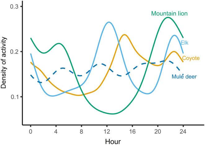
Density of activity (i.e., movement rate) of elk, coyotes, and mountain lions across a 24‐h period developed from GPS data collected from 1 May to 1 September in 2018 and 2019 in southwest Wyoming, USA.

FIGURE 3.

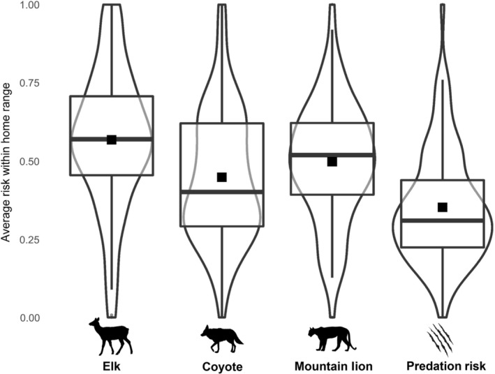
Violin plots displaying variation across all deer in the average value of probability of encounter with elk, coyotes, and mountain lions and risk of predation within home ranges of female deer. Furthermore, box plots are overlaid to illustrate minimum, maximum, and quartile ranges for average value of risk across all deer. Mean for each risk factor for all deer is displayed as a black square.

Movement activity and spatial risk

We evaluated four linear models, one for each risk metric (i.e., probability of encounter with elk, coyotes, and mountain lions, and risk of predation), to test relationships between overlap in activity and the average exposure to risk within home ranges of deer. Deer did not reduce overlap in activity with elk, coyotes, or mountain lions or predation risk as the average exposure to risk of encounter increased within their home range (p values > 0.05; Figure 4).

FIGURE 4.

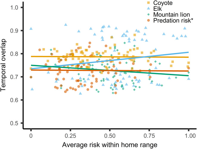
Regression lines from linear models of temporal overlap with elk, coyotes, and mountain lions by female mule deer in response to the average value of risk within home ranges of female deer (i.e., temporal functional response). Points illustrate observations of average value within home ranges and temporal overlap of each female deer‐year combination (n = 65), and corresponding source of risk. We did not detect an effect of the average value of risk from elk, coyotes, mountain lions, or predation risk within home ranges on temporal activity of female deer (p > 0.05).

Step‐selection functions

Across our four model sets, the functional response model, which included the interaction term between spatial variation in risk (i.e., probability of encounter or risk of predation) and the average value of risk within deer home ranges was our top selected model for all risk factors except coyotes (Table 2). Support for the space‐only and space × time models was substantially weaker than the top models including a spatial functional response for elk, mountain lions, and predation risk (Table 2). In contrast, the best‐fit model for encounter with coyotes was the space‐only model that included only the probability of use by coyotes, however, model fit was worse than the global model (space‐only = 2,238,742, global = 2,238,730; Table 2). Given that our aim was to compare behavior of deer across multiple forms of risk, we elected to interpret the coefficients from the space‐only model for coyotes.

TABLE 2.

All models from step‐selection functions to evaluate fine‐scale behaviors of female deer relative to the risk of encounter with elk, coyotes, and mountain lions, and the risk of predation by mountain lions in southwest Wyoming, USA from 2018 to 2019.

Risk metric/Model	K	QIC	ΔQIC
Elk
SPACE × HR EXPOSURE	13	2,237,550	0.0
SPACE‐ONLY	12	2,238,351	801.0
SPACE × TIME	13	2,238,394	844.0
Coyote
SPACE‐ONLY	12	2,238,742	0.0
SPACE × HR EXPOSURE	13	2,238,762	20.0
SPACE × TIME	13	2,238,791	49.0
Mountain lion
SPACE × HR EXPOSURE	13	2,238,111	0.0
SPACE × TIME	13	2,238,593	482.0
SPACE‐ONLY	12	2,238,619	508.0
Predation risk
SPACE × HR EXPOSURE	13	2,238,182	0.0
SPACE‐ONLY	12	2,238,497	315.0
SPACE × TIME	13	2,238,507	325.0

Notes: Models were evaluated based on quasi‐likelihood Independence criterion (QIC), and ΔQIC; we also provide the number of parameters (K) for each model. QIC for the global model was 2,238,730.

Across all models with the four risk factors, the best overall was the functional response model that incorporated probability of encounter with elk, which improved QIC by 561 from the next best model (i.e., probability of encounter with mountain lions × average within home range; Table 2). Deer took steps that were indifferent to distance to primary and secondary roads, topographic position index, and percent annual forb cover (Table 3).

TABLE 3.

Coefficients of the effects of landscape variables and risk metrics on fine‐scale selection by female mule deer as expressed by odds ratios (OR) and 95% confidence intervals based on robust standards errors of top‐ranked model within each risk metric.

Parameter	Elk			Coyote			Mountain lion			Predation risk
		95% CI			95% CI			95% CI			95% CI
	OR	Lower	Upper	OR	Lower	Upper	OR	Lower	Upper	OR	Lower	Upper
COSTA	0.991	0.985	0.997	0.991	0.985	0.996	0.991	0.985	0.997	0.991	0.985	0.997
ELEV	0.736	0.621	0.871	0.735	0.628	0.861	0.721	0.620	0.839	0.735	0.630	0.816859
SHRUB	1.381	1.106	1.723	1.500	1.213	1.855	1.462	1.177	1.814	1.402	1.134	1.732
FOREST	1.864	1.485	2.341	2.238	1.795	2.790	1.9940	1.519	2.480	2.0.018	1.621	2.512
TRI	1.594	1.326	1.916	1.652	1.383	1.975	1.376	1.125	1.684	1.590	1.345	1.880
LITTER	0.737	0.627	0.865	0.726	0.623	0.845	0.745	0.639	0.868	0.736	0.633	0.856
PERENN	1.316	1.053	1.644	1.529	1.260	1.857	1.543	1.274	1.868	1.480	1.212	1.808
SPATIAL RISK	1.996	1.681	2.370	…	…	…	1.824	1.557	2.138	4.837	3.360	6.964
SPATIAL RISK × HR	0.534	0.449	0.636	X	X	X	0.522	0.421	0.648	0.093	0.036	0.240

Notes: An “X” indicates that the parameter was not present within the top model; only parameters that were significant are presented. Parameters include elevation (ELEV), percent SHRUB cover (SHRUB), percent forest cover (TREE), terrain ruggedness index (TRI), percent LITTER cover (LITTER), and percent perennial cover (PERENN) as well as our metric of SPATIAL RISK (SPATIAL RISK) and the interaction between spatial risk and exposure within home ranges (HR).

Deer took steps towards higher probability of use by elk and mountain lions, however, the strength of selection was dampened as the average level of exposure to elk and mountain lions increased. For instance, the odds of taking steps towards the risk of encountering an elk decreased from 1.47 to 1.0 when the average exposure of elk within deer home ranges increased from 0.45 (25th percentile) to 0.68 (75th percentile), respectively (Figure 5). Similarly, the odds of taking steps towards the risk of encountering a mountain lion decreased from 1.35 to 1.02 when the average exposure to mountain lions within home ranges increased from 0.39 (25th percentile) to 0.64 (75th percentile), respectively (Figure 5).

FIGURE 5.

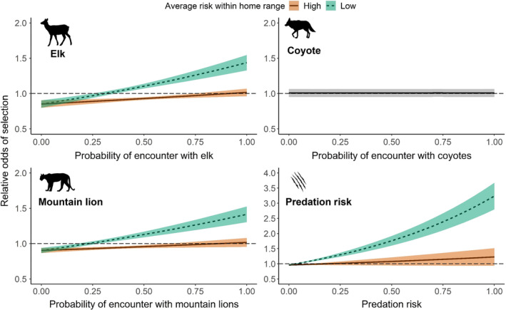
Predicted responses of female deer to the probability of encounter with elk, coyotes, mountain lions, and predation risk relative to average exposure within home ranges. Categories of exposure (low vs. high) were based on 75th percentile of exposure to risk within home ranges of female deer; any values below the 25th percentile were classified as “low” exposure whereas all value above the 75th percentile were classified as “high” exposure. The gray panel (top right) illustrates the relationship between space use by coyotes and probability of selection by female deer. Note the axis for predation risk is about two times that of elk, coyotes, and mountain lions. Horizontal dashed lines indicate threshold of selection for odds ratios (i.e., 1.0).

Females exhibited the strongest behavioral response to predation risk. An area on the landscape that was predicted as a kill site was 4.8 times more likely to be selected by deer than a place that was not a kill site (Table 3). Nevertheless, females were less likely to select for increased predation risk when the average level of predation risk within their home ranges was high (Figure 5). For example, the odds of moving towards predation risk decreased from 3.15 to 1.25 when the average exposure to predation risk within deer home ranges increased from 0.22 (25th percentile) to 0.42 (75th percentile) (Figure 5). Deer were indifferent towards increasing risk of encounter with coyotes (Figure 5).

DISCUSSION

In heterogeneous environments, animals are tasked with securing energetic resources while navigating multiple, competing risks across the landscape. Whether in the form of a nutritional loss or direct risk of mortality, deer presumably did not spatially avoid risk at a fine scale within their home ranges and made movement steps that increased risk of encountering elk and mountain lions as well as the risk of predation by mountain lions. Positive selection for predation risk by deer is likely implicit for a couple of reasons. First, deer likely do not have perfect knowledge of predation risk, and decisions made to avoid the risk of predation may result in trade‐offs associated with nutritional demands or movement constraints associated with fawn rearing (Long et al., 2009; Singh & Ericsson, 2014). Second, in our system, mountain lions are required to select areas where deer occur, which is consistent with their diet composition. Under these circumstances, we should expect deer to exhibit some level of affinity towards predation risk, even though it may be in part a function of predators selecting deer habitat. Contrary to findings from similar studies, deer did not shift activity patterns based on activity peaks of competitors and predators (e.g., elk, coyotes, and mountain lions; Courbin et al., 2019; Kohl et al., 2018, 2019; Smith et al., 2019; Tambling et al., 2015). Deer responded to spatial risk in a context‐dependent framework, and lowered their selection for risky places (i.e., high probability of encounter or risk of predation) when the average level of risk within their home range was high (Figure 5). The similar activity patterns across deer, elk, coyotes, and mountain lions, coupled with strong selection for areas of high probability of use by elk, mountain lions, and risk of predation, highlights a reduced plasticity for deer in our desert environment. These findings underscore the importance of considering context‐dependent decisions of prey in a world where risk is multidimensional across both space and time (Holbrook et al., 2017, 2019; Mason & Fortin, 2017; Ross et al., 2013; Tambling et al., 2015).

A main aim of ecology is understanding the factors that influence resource selection and movement of animals (Holbrook et al., 2019; Mason & Fortin, 2017). Consequently, ecologists and managers target efforts to identify, predict, and understand distributions of animals across the landscape, and the many variables that underpin that distribution (Holbrook et al., 2017). Issues may arise, however, when animal behavior (e.g., habitat selection) is assumed to remain constant with respect to changing conditions (Holbrook et al., 2017, 2019; Mason & Fortin, 2017). Environmental conditions are not static, but rather fluid attributes wherein resources and risk are variable across space and time (Aikens et al., 2017; Dwinnell et al., 2019; Pierce et al., 2004). Considering functional responses (i.e., selection varies according to availability or exposure) may be crucial to reveal the context‐dependent nature of how animals respond to the risks that they are exposed to within their environment. Deer selected strongly for risky places within their home ranges, and did not shift space use relative to times when risk was presumably greatest (i.e., activity peaks of elk, coyotes, and mountain lions); instead, the response of deer was strongly mediated by the average amount of risk they experienced within their home ranges (Figure 5). Ignoring functional responses in selection would have led to the conclusion that deer selected for risk and did nothing to mitigate their exposure to risk within their home range.

Movement decisions of animals emerge from responses to their environment and the internal state of the animal that determines where and how to move (Latombe et al., 2011; Mason & Fortin, 2017; Nathan et al., 2008). Consequently, resource availability and distribution of risk should affect movement decisions made by animals. Predators on the landscape actively target areas where encounters with prey are likely (Mason & Fortin, 2017; Sih, 2000), while simultaneously, prey exhibit avoidance responses to certain habitat features that represent greater risk. Nevertheless, prey should respond to risk within their local environment by selecting for “safe” patches. For “safe” patches to be available to an animal, food resources should be spatially disconnected from the distribution of risk. In situations where high‐quality resources are relatively constrained in space, such as in desert environments, it may be easier for a predator to align their spatial distribution with the distribution of prey species. Under these circumstances, it may be difficult for prey to entirely avoid risky places because of these environmental constraints. This context may explain why we observed deer exhibiting such strong selection for most forms of risk (i.e., probability of encounter with elk and mountain lions and predation risk) within our high‐desert environment. Our analyses of fine‐scale movement decisions made by deer relative to multiple, contrasting risks indicate that deer make spatial adjustments in response to their local environment, potentially as the only tactic available to mitigate risk.

We evaluated multiple dimensions of risk posed to deer across space and time (i.e., probability of encounter with elk, coyotes, and mountain lions and predation risk). We incorporated metrics of movement activity patterns (i.e., temporal overlap) and spatial variation in the distribution of elk, coyotes, and mountain lions, as well as the risk of predation by mountain lions. Unlike other work, however, we added spatial variation in risk of encountering a potential competitor on the landscape. The summer months from May to September represent a period of time wherein female ungulates face the greatest nutritional demands, most notably provisioning young while building fat stores for the winter (Cook et al., 2004; Monteith et al., 2013). Consequently, interactions with a potential competitor (i.e., nutritional losses) during summer could be detrimental to survival of adult females. Although our results do not necessarily point to competition itself as a demographic force underlying selection by deer, deer selected for increased probability of encounter with elk, but did so less strongly when the average probability of encountering elk increased. Nevertheless, interactions with a potential competitor are often only one form of risk that some species are striving to balance, especially when other forms of risk can result in direct mortality.

Our results are somewhat contradictory to current literature that exists on responses of prey relative to spatiotemporal variation in risk, perhaps for a number of reasons. First, most work has used proxies of risk, meaning that habitat features were used to represent spatial variation in risk (Kohl et al., 2019; Smith et al., 2019). For instance, roughness and vegetation openness were used to represent hunting domains of mountain lions and wolves, respectively, and female elk selected for rough terrain when mountain lion activity was low and selected for open terrain when wolf activity was high (Kohl et al., 2019). Proxies of risk, however, may not be applicable in situations where a single habitat feature does not align with risk. For example, predators that have heterogeneous hunting domains (e.g., high vegetation cover on flat terrain or high topographic variation with little vegetation) may not invoke specific responses of prey based on a single habitat feature (Smith et al., 2019). Consequently, evaluating the responses of prey solely through the lens of habitat attributes instead of the lens of space use of a predator may result in divergent patterns of prey behavior relative to how risk is quantified. We modeled probability of encounter of elk, coyotes, and mountain lions, as well as the risk of predation, across the landscape with empirical data that incorporated many habitat features to produce a single composite layer through the lens of each risk factor. Therefore, our results are directly comparable to spatial variation in risk and provide the necessary context to understand prey behavior relative to the spatial distribution of risk.

Second, temporal variation in risk (i.e., movement activity patterns) has been identified as an important component driving prey behavior (Courbin et al., 2019; Kohl et al., 2018, 2019; Smith et al., 2019; Tambling et al., 2015), contrary to our findings. Deer in our study had the opportunity to shift activity to midday, which would have minimized interactions with all forms of risk, however, temporal overlap in activity of deer with elk, coyotes, and mountain lions was high (Figure 2). The majority of work regarding spatiotemporal variation in risk has used population‐level movement rates (m/h) as the metric to represent diel activity patterns (Kohl et al., 2018; Smith et al., 2019), whereas we used coefficient of overlap. Using coefficient of overlap as the metric for temporal activity allowed us to identify individual‐level shifts in activity, and how those shifts varied across a gradient in spatial exposure to risk within deer home ranges.

Biological clocks of animals determine activity patterns throughout a daily period, and may not be plastic enough to facilitate major changes outside of peak activity periods, especially in herbivores who live in relatively stable climatic conditions, and are not likely affected by ephemeral feeding opportunities (Bartness & Elliott Albers, 2000; Bloch et al., 2013). In response to the demands of late gestation and peak lactation, however, reproductive females may be required to forage during all hours of the day (Hamel & Côté, 2009). Despite the potential need to forage during the middle of the day, deer in our system did not shift their activity as indexed through movement rates. Thermal constraints that are present during the middle of the day may outweigh the benefits of shifting activity to avoid biotic interactions or forage gain to support the demands of lactation (Owen‐Smith, 1998; van Beest & Milner, 2013). Consequently, deer may not have the opportunity to alter peak activity to reduce risk from predation and potential competition, or alternatively they are choosing to minimize the risk of thermal exposure at the cost of temporal exposure with predators and a competitor. Ultimately, our results support the notion that deer do not modulate activity patterns to avoid risk, rather they mitigate risk by considering gradients in the spatial distribution of risk as well as the amount of risk they are exposed to within their home range.

Deer in our high‐desert system were unable to avoid risk within home ranges when exposed to the presence of two predators and a potential competitor, however, they attempted to make the best of their circumstance by mediating selection relative to the amount of risk they were exposed to within their home ranges. Animals are faced with balancing the needs of acquiring resources necessary for survival with risk of direct mortality to themselves and their offspring. In systems where risk is one‐dimensional, animals should choose to avoid that risk if that risk poses a detriment to survival. Single dimensions of risk, however, are rare in most systems. Prey are often faced with risk factors that are multidimensional and can affect fitness through different pathways (e.g., direct mortality or nutritional loss). Consequently, shifts in behavior, whether in space use or activity patterns, are the primary mechanisms by which prey mediate risk across the landscape. Such shifts may not be the end‐all solution to eliminating risk when multiple, competing risks exist. Prey might be faced with the need to minimize risk in a contextual framework based on local availability. Our analyses highlight the importance of accounting for local environmental conditions when identifying the effects of predation risk and competitive interactions on animal behavior. Moreover, our work exposes additional behavioral mechanisms prey species might employ to mitigate risk to their survival, especially in systems where risk is multi‐fold.

CONFLICT OF INTEREST

The authors declare there are no conflicts of interest.

Supporting information

Appendix S1

Appendix S2

Huggler, Katey S. , Holbrook Joseph D., Hayes Matthew M., Burke Patrick W., Zornes Mark, Thompson Daniel J., Clapp Justin G., Lionberger Patrick, Valdez Miguel, and Monteith Kevin L.. 2022. “Risky Business: How an Herbivore Navigates Spatiotemporal Aspects of Risk from Competitors and Predators.” Ecological Applications 32(7): e2648. 10.1002/eap.2648

DATA AVAILABILITY STATEMENT

Data (Huggler et al., 2022) are available in Dryad at https://doi.org/10.5061/dryad.0rxwdbs2w.

REFERENCES

- Aikens, E. O. , Kauffman M. J., Merkle J. A., Dwinnell S. P. H., Fralick G. L., and Monteith K. L.. 2017. “The Greenscape Shapes Surfing of Resource Waves in a Large Migratory Herbivore.” Ecology Letters 20(6): 741–50. 10.1111/ELE.12772. [DOI] [PubMed] [Google Scholar]
- Altendorf, K. B. , Laundré J. W., López González C. A., and Brown J. S.. 2001. “Assessing Effects of Predation Risk on Foraging Behavior of Mule Deer.” Journal of Mammalogy 82(2): 430–9. [Google Scholar]
- Avgar, T. , Potts J. R., Lewis M. A., and Boyce M. S.. 2016. “Integrated Step Selection Analysis: Bridging the Gap between Resource Selection and Animal Movement.” Methods in Ecology and Evolution 7(5): 619–30. 10.1111/2041-210X.12528. [DOI] [Google Scholar]
- Barrett, M. W. , Nolan J. W., and Roy L. D.. 1982. “Evaluation of a Hand‐Held Net‐Gun to Capture Large Mammals on JSTOR.” Wildlife Society Bulletin. 10(2): 108–14 https://www.jstor.org/stable/3781727?seq=1. [Google Scholar]
- Bartness, T. J. , and Elliott Albers H.. 2000. “Activity Patterns and the Biological Clock in Mammals.” In Activity Patterns in Small Mammals. Ecological Studies, Vol 141, edited by Halle S. and Stenseth N. C., 23–47. Berlin: Springer. 10.1007/978-3-642-18264-8_3. [DOI] [Google Scholar]
- Benhamou, S. 2004. “How to Reliably Estimate the Tortuosity of an Animal's Path:: Straightness, Sinuosity, or Fractal Dimension?” Journal of Theoretical Biology 229(2): 209–20. 10.1016/J.JTBI.2004.03.016. [DOI] [PubMed] [Google Scholar]
- Bergerud, A. T. , and Page R. E.. 2011. “Displacement and Dispersion of Parturient Caribou at Calving as Antipredator Tactics.” Canadian Journal of Zoology 65(7): 1597–606. 10.1139/Z87-249. [DOI] [Google Scholar]
- Bergman, C. M. , Fryxell J. M., Cormack Gates C., and Fortin D.. 2001. “Ungulate Foraging Strategies: Energy Maximizing or Time Minimizing?” Journal of Animal Ecology 70(2): 289–300. 10.1111/J.1365-2656.2001.00496.X. [DOI] [Google Scholar]
- Bloch, G. , Barnes B. M., Gerkema M. P., and Helm B.. 2013. “Animal Activity around the Clock with no Overt Circadian Rhythms: Patterns, Mechanisms and Adaptive Value.” Proceedings of the Royal Society B: Biological Sciences 280(1765): 20130019. 10.1098/RSPB.2013.0019. [DOI] [PMC free article] [PubMed] [Google Scholar]
- Bøving, P. S. , and Post E.. 1997. “Vigilance and Foraging Behaviour of Female Caribou in Relation to Predation Risk.” Rangifer 17(2): 55–63. 10.7557/2.17.2.1302. [DOI] [Google Scholar]
- Bowen, W. D. 1982. “Home Range and Spatial Organization of Coyotes in Jasper National Park, Alberta.” The Journal of Wildlife Management 46(1): 201. 10.2307/3808423. [DOI] [Google Scholar]
- Bowyer, R. T. , McCullough D. R., and Belovsky G. E.. 2001. “Causes and Consequences of Sociality in Mule Deer.” Alces 37(2): 371–402. [Google Scholar]
- Breiman, L. 2001. “Random Forests.” Machine Learning 45(1): 5–32. 10.1023/A:1010933404324. [DOI] [Google Scholar]
- Brown, J. S. 1988. “Patch Use as an Indicator of Habitat Preference, Predation Risk, and Competition.” Behavioral Ecology and Sociobiology 22(1): 37–47. 10.1007/BF00395696. [DOI] [Google Scholar]
- Brown, J. S. 1999. “Vigilance, Patch Use and Habitat Selection: Foraging under Predation Risk.” Evolutionary Ecology Research 1: 49–71. [Google Scholar]
- Brown, J. S. , and Kotler B. P.. 2004. “Hazardous Duty Pay and the Foraging Cost of Predation.” Ecology Letters 7(10): 999–1014. 10.1111/J.1461-0248.2004.00661.X. [DOI] [Google Scholar]
- Cook, J. G. , Johnson B. K., Cook R. C., Riggs R. A., Delcurto T., Bryant L. D., and Irwin L. L.. 2004. “Effects of Summer‐Autumn Nutrition and Parturition Date on Reproduction and Survival of Elk.” Wildlife Monographs 155: 1–63. 10.2193/0084-0173. [DOI] [Google Scholar]
- Courbin, N. , Loveridge A. J., Fritz H., Macdonald D. W., Patin R., Valeix M., and Chamaillé‐Jammes S.. 2019. “Zebra Diel Migrations Reduce Encounter Risk with Lions at Night.” Journal of Animal Ecology 88(1): 92–101. 10.1111/1365-2656.12910. [DOI] [PubMed] [Google Scholar]
- Cowlishaw, G. 1997. “Trade‐Offs between Foraging and Predation Risk Determine Habitat Use in a Desert Baboon Population.” Animal Behaviour 53(4): 667–86. 10.1006/ANBE.1996.0298. [DOI] [PubMed] [Google Scholar]
- Crawford, D. A. , Mike Conner L., Morris G., and Cherry M. J.. 2021. “Predation Risk Increases Intraspecific Heterogeneity in White‐Tailed Deer Diel Activity Patterns.” Behavioral Ecology 32(1): 41–8. 10.1093/BEHECO/ARAA089. [DOI] [Google Scholar]
- Creel, S. , Schuette P., and Christianson D.. 2014. “Effects of Predation Risk on Group Size, Vigilance, and Foraging Behavior in an African Ungulate Community.” Behavioral Ecology 25(4): 773–84. 10.1093/BEHECO/ARU050. [DOI] [Google Scholar]
- Creel, S. , and Winnie J. A.. 2005. “Responses of Elk Herd Size to Fine‐Scale Spatial and Temporal Variation in the Risk of Predation by Wolves.” Animal Behaviour 69(5): 1181–9. 10.1016/J.ANBEHAV.2004.07.022. [DOI] [Google Scholar]
- Crosmary, W. G. , Valeix M., Fritz H., Madzikanda H., and Côté S. D.. 2012. “African Ungulates and their Drinking Problems: Hunting and Predation Risks Constrain Access to Water.” Animal Behaviour 83(1): 145–53. 10.1016/J.ANBEHAV.2011.10.019. [DOI] [Google Scholar]
- Cusack, J. J. , Kohl M. T., Metz M. C., Coulson T., Stahler D. R., Smith D. W., and MacNulty D. R.. 2020. “Weak Spatiotemporal Response of Prey to Predation Risk in a Freely Interacting System.” Journal of Animal Ecology 89(1): 120–31. 10.1111/1365-2656.12968. [DOI] [PMC free article] [PubMed] [Google Scholar]
- Dwinnell, S. P. H. , Sawyer H., Randall J. E., Beck J. L., Forbey J. S., Fralick G. L., and Monteith K. L.. 2019. “Where to Forage when Afraid: Does Perceived Risk Impair Use of the Foodscape?” Ecological Applications 29(7): e01972. 10.1002/EAP.1972. [DOI] [PMC free article] [PubMed] [Google Scholar]
- Ensing, E. P. , Ciuti S., de Wijs F. A. L. M., Lentferink D. H., Hoedt A., Boyce M. S., and Hut R. A.. 2014. “GPS Based Daily Activity Patterns in European Red Deer and North American Elk (Cervus Elaphus): Indication for a Weak Circadian Clock in Ungulates.” PLoS One 9(9): e106997. 10.1371/JOURNAL.PONE.0106997. [DOI] [PMC free article] [PubMed] [Google Scholar]
- Fortin, D. , Beyer H. L., Boyce M. S., Smith D. W., Duchesne T., and Mao J. S.. 2005. “Wolves Influence Elk Movements: Behavior Shapes A Trophic Cascade in Yellowstone National Park.” Ecology 86(5): 1320–30. 10.1890/04-0953. [DOI] [Google Scholar]
- Frair, J. L. , Merrill E. H., Visscher D. R., Fortin D., Beyer H. L., and Morales J. M.. 2005. “Scales of Movement by Elk (Cervus elaphus) in Response to Heterogeneity in Forage Resources and Predation Risk.” Landscape Ecology 20(3): 273–87. 10.1007/S10980-005-2075-8. [DOI] [Google Scholar]
- Gaillard, J. M. , Hebblewhite M., Loison A., Fuller M., Powell R., Basille M., and van Moorter B.. 2010. “Habitat–Performance Relationships: Finding the Right Metric at a Given Spatial Scale.” Philosophical Transactions of the Royal Society B: Biological Sciences 365(1550): 2255–65. 10.1098/RSTB.2010.0085. [DOI] [PMC free article] [PubMed] [Google Scholar]
- Gaynor, K. M. 2019. Spatial and Temporal Responses of Animals to Landscape Heterogeneity, Predation Risk, and Human Activity ‐ ProQuest. Berkeley: UC Berkeley; https://www.proquest.com/openview/c49c810677f349b411efcf0a4d943c6c/1?pq-origsite=gscholar&cbl=18750&diss=y. [Google Scholar]
- Gervasi, V. , Sand H., Zimmermann B., Mattisson J., Wabakken P., and Linnell J. D. C.. 2013. “Decomposing Risk: Landscape Structure and Wolf Behavior Generate Different Predation Patterns in Two Sympatric Ungulates.” Ecological Applications 23(7): 1722–34. 10.1890/12-1615.1. [DOI] [PubMed] [Google Scholar]
- Gier, H. T. 1957. Coyotes in Kansas. Manhattan, KS: Kansas Sate College of Agricultural and Applied Science. [Google Scholar]
- Grant, J. , Hopcraft C., Sinclair A. R. E., and Packer C.. 2005. “Planning for Success: Serengeti Lions Seek Prey Accessibility Rather than Abundance.” Journal of Animal Ecology 74(3): 559–66. 10.1111/J.1365-2656.2005.00955.X. [DOI] [Google Scholar]
- Hamel, S. , and Côté S. D.. 2009. “Maternal Defensive Behavior of Mountain Goats against Predation by Golden Eagles.” Western North American Naturalist 69(1): 115–8. 10.3398/064.069.0103. [DOI] [Google Scholar]
- Hebblewhite, M. , Merrill E. H., and McDonald T. L.. 2005. “Spatial Decomposition of Predation Risk Using Resource Selection Functions: An Example in a Wolf–Elk Predator–Prey System.” Oikos 111(1): 101–11. 10.1111/J.0030-1299.2005.13858.X. [DOI] [Google Scholar]
- Holbrook, J. D. , Olson L. E., DeCesare N. J., Hebblewhite M., Squires J. R., and Steenweg R.. 2019. “Functional Responses in Habitat Selection: Clarifying Hypotheses and Interpretations.” Ecological Applications 29(3): e01852. 10.1002/EAP.1852. [DOI] [PubMed] [Google Scholar]
- Holbrook, J. D. , Squires J. R., Olson L. E., Decesare N. J., and Lawrence R. L.. 2017. “Understanding and Predicting Habitat for Wildlife Conservation: The Case of Canada Lynx at the Range Periphery.” Ecosphere 8(9): e01939. 10.1002/ECS2.1939. [DOI] [Google Scholar]
- Huggler, K. , Holbrook J., Hayes M., Burke P., Zornes M., Thompson D., Clapp J., Lionberger P., Valdez M., and Monteith K.. 2022. “Risky Business: How an Herbivore Navigates Spatio‐Temporal Aspects of Risk from Competitors and Predators.” Dryad, Dataset. 10.5061/dryad.0rxwdbs2w. [DOI] [PMC free article] [PubMed]
- Hugie, D. M. , and Dill L. M.. 1994. “Fish and Game: A Game Theoretic Approach to Habitat Selection by Predators and Prey.” Journal of Fish Biology 45: 151–69. 10.1111/J.1095-8649.1994.TB01090.X. [DOI] [Google Scholar]
- Johnson, B. K. , Kern J. W., Wisdom M. J., Findholt S. L., and Kie J. G.. 2000. “Resource Selection and Spatial Separation of Mule Deer and Elk during Spring.” The Journal of Wildlife Management 64(3): 685. 10.2307/3802738. [DOI] [Google Scholar]
- Johnson, C. J. , Seip D. R., and Boyce M. S.. 2004. “A Quantitative Approach to Conservation Planning: Using Resource Selection Functions to Map the Distribution of Mountain Caribou at Multiple Spatial Scales.” Journal of Applied Ecology 41(2): 238–51. 10.1111/J.0021-8901.2004.00899.X. [DOI] [Google Scholar]
- Jones, M. O. , Allred B. W., Naugle D. E., Maestas J. D., Donnelly P., Metz L. J., Karl J., et al. 2018. “Innovation in Rangeland Monitoring: Annual, 30 m, Plant Functional Type Percent Cover Maps for U.S. Rangelands, 1984–2017.” Ecosphere 9(9): e02430. 10.1002/ECS2.2430. [DOI] [Google Scholar]
- Kacelnik, A. , Krebs J. R., and Bernstein C.. 1992. “The Ideal Free Distribution and Predator‐Prey Populations.” Trends in Ecology & Evolution 7(2): 50–5. 10.1016/0169-5347(92)90106-L. [DOI] [PubMed] [Google Scholar]
- Kauffman, M. J. , Varley N., Smith D. W., Stahler D. R., MacNulty D. R., and Boyce M. S.. 2007. “Landscape Heterogeneity Shapes Predation in a Newly Restored Predator–Prey System.” Ecology Letters 10(8): 690–700. 10.1111/J.1461-0248.2007.01059.X. [DOI] [PubMed] [Google Scholar]
- Kie, J. G. 2013. “A Rule‐Based Ad Hoc Method for Selecting a Bandwidth in Kernel Home‐Range Analyses.” Animal Biotelemetry 1(1): 1–12. 10.1186/2050-3385-1-13/TABLES/1. [DOI] [Google Scholar]
- Kie, J. G. , Matthiopoulos J., Fieberg J., Powell R. A., Cagnacci F., Mitchell M. S., Gaillard J. M., and Moorcroft P. R.. 2010. “The Home‐Range Concept: Are Traditional Estimators Still Relevant with Modern Telemetry Technology?” Philosophical Transactions of the Royal Society B: Biological Sciences 365(1550): 2221–31. 10.1098/RSTB.2010.0093. [DOI] [PMC free article] [PubMed] [Google Scholar]
- Kohl, M. T. , Ruth T. K., Metz M. C., Stahler D. R., Smith D. W., White P. J., and MacNulty D. R.. 2019. “Do Prey Select for Vacant Hunting Domains to Minimize a Multi‐Predator Threat?” Ecology Letters 22(11): 1724–33. 10.1111/ELE.13319. [DOI] [PubMed] [Google Scholar]
- Kohl, M. T. , Stahler D. R., Metz M. C., Forester J. D., Kauffman M. J., Varley N., White P. J., Smith D. W., and Macnulty D. R.. 2018. “Diel Predator Activity Drives a Dynamic Landscape of Fear.” Ecological Monographs 88(4): 638–52. [Google Scholar]
- Lashley, M. A. , Cove M. V., Chitwood M. C., Penido G., Gardner B., Deperno C. S., and Moorman C. E.. 2018. “Estimating Wildlife Activity Curves: Comparison of Methods and Sample Size.” Scientific Reports 8(1): 1–11. 10.1038/s41598-018-22638-6. [DOI] [PMC free article] [PubMed] [Google Scholar]
- Latombe, G. , Parrott L., and Fortin D.. 2011. “Levels of Emergence in Individual Based Models: Coping with Scarcity of Data and Pattern Redundancy.” Ecological Modelling 222(9): 1557–68. 10.1016/J.ECOLMODEL.2011.02.020. [DOI] [Google Scholar]
- Lima, S. L. 1992. “Strong Preferences for Apparently Dangerous Habitats? A Consequence of Differential Escape from Predators.” Oikos 64(3): 597. 10.2307/3545181. [DOI] [Google Scholar]
- Lima, S. L. 1998. “Nonlethal Effects in the Ecology of Predator‐Prey Interactions.” Bioscience 48(1): 25–34. 10.2307/1313225. [DOI] [Google Scholar]
- Lone, K. , Loe L. E., Gobakken T., Linnell J. D. C., Odden J., Remmen J., Mysterud A., et al. 2014. “Living and Dying in a Multi‐Predator Landscape of Fear: Roe Deer Are Squeezed by Contrasting Pattern of Predation Risk Imposed by Lynx and Humans.” Oikos 123(6): 641–51. 10.1111/J.1600-0706.2013.00938.X. [DOI] [Google Scholar]
- Long, R. A. , Kie J. G., Terry Bowyer R., and Hurley M. A.. 2009. “Resource Selection and Movements by Female Mule Deer Odocoileus hemionus: Effects of Reproductive Stage.” Wildlife Biology 15(3): 288–98. 10.2981/09-003. [DOI] [Google Scholar]
- Long, R. A. , Terry Bowyer R., Porter W. P., Mathewson P., Monteith K. L., and Kie J. G.. 2014. “Behavior and Nutritional Condition Buffer a Large‐Bodied Endotherm against Direct and Indirect Effects of Climate.” Ecological Monographs 84(3): 513–32. 10.1890/13-1273.1. [DOI] [Google Scholar]
- Mason, T. H. E. , and Fortin D.. 2017. “Functional Responses in Animal Movement Explain Spatial Heterogeneity in Animal–Habitat Relationships.” Journal of Animal Ecology 86(4): 960–71. 10.1111/1365-2656.12682. [DOI] [PubMed] [Google Scholar]
- Merems, J. L. , Shipley L. A., Levi T., Ruprecht J., Clark D. A., Wisdom M. J., Jackson N. J., Stewart K. M., and Long R. A.. 2020. “Nutritional‐Landscape Models Link Habitat Use to Condition of Mule Deer (Odocoileus hemionus).” Frontiers in Ecology and Evolution 8(April): 98. 10.3389/fevo.2020.00098. [DOI] [Google Scholar]
- Middleton, A. D. , Kauffman M. J., Mcwhirter D. E., Jimenez M. D., Cook R. C., Cook J. G., Albeke S. E., Sawyer H., and White P. J.. 2013. “Linking Anti‐Predator Behaviour to Prey Demography Reveals Limited Risk Effects of an Actively Hunting Large Carnivore.” Ecology Letters 16(8): 1023–30. 10.1111/ELE.12133. [DOI] [PubMed] [Google Scholar]
- Mills, D. R. , do Linh San E., Robinson H., Isoke S., Slotow R., and Hunter L.. 2019. “Competition and Specialization in an African Forest Carnivore Community.” Ecology and Evolution 9(18): 10092–108. 10.1002/ECE3.5391. [DOI] [PMC free article] [PubMed] [Google Scholar]
- Moll, R. J. , Redilla K. M., Mudumba T., Muneza A. B., Gray S. M., Abade L., Hayward M. W., Millspaugh J. J., and Montgomery R. A.. 2017. “The Many Faces of Fear: A Synthesis of the Methodological Variation in Characterizing Predation Risk.” Journal of Animal Ecology 86(4): 749–65. 10.1111/1365-2656.12680. [DOI] [PubMed] [Google Scholar]
- Monteith, K. L. , Bleich V. C., Stephenson T. R., Pierce B. M., Conner M. M., Kie J. G., and Terry Bowyer R.. 2014. “Life‐History Characteristics of Mule Deer: Effects of Nutrition in a Variable Environment.” Wildlife Monographs 186(1): 1–62. 10.1002/WMON.1011. [DOI] [Google Scholar]
- Monteith, K. L. , Sexton C. L., Jenks J. A., and Terry Bowyer R.. 2007. “Evaluation of Techniques for Categorizing Group Membership of White‐Tailed Deer.” The Journal of Wildlife Management 71(5): 1712–6. 10.2193/2005-763. [DOI] [Google Scholar]
- Monteith, K. L. , Stephenson T. R., Bleich V. C., Conner M. M., Pierce B. M., and Terry Bowyer R.. 2013. “Risk‐Sensitive Allocation in Seasonal Dynamics of Fat and Protein Reserves in a Long‐Lived Mammal.” Journal of Animal Ecology 82(2): 377–88. 10.1111/1365-2656.12016. [DOI] [PubMed] [Google Scholar]
- Nathan, R. , Getz W. M., Revilla E., Holyoak M., Kadmon R., Saltz D., and Smouse P. E.. 2008. “A Movement Ecology Paradigm for Unifying Organismal Movement Research.” Proceedings of the National Academy of Sciences USA 105(49): 19052–9. 10.1073/PNAS.0800375105/SUPPL_FILE/APPENDIX_PDF.PDF. [DOI] [PMC free article] [PubMed] [Google Scholar]
- Northrup, J. M. , Anderson C. R., Hooten M. B., and Wittemyer G.. 2016. “Movement Reveals Scale Dependence in Habitat Selection of a Large Ungulate.” Ecological Applications 26(8): 2746–57. 10.1002/EAP.1403. [DOI] [PubMed] [Google Scholar]
- Oliveira‐Santos, G. , Luiz R., Eletrosul C. A. Z., Oliveira‐Santos L. G. R., Zucco C. A., and Agostinelli C.. 2012. “Using Conditional Circular Kernel Density Functions to Test Hypotheses on Animal Circadian Activity.” Animal Behaviour 85(1): 269–80. 10.1016/j.anbehav.2012.09.033. [DOI] [Google Scholar]
- Owen‐Smith, N. 1998. “How High Ambient Temperature Affects the Daily Activity and Foraging Time of a Subtropical Ungulate, the Greater Kudu (Tragelaphus strepsiceros).” Journal of Zoology 246(2): 183–92. 10.1111/J.1469-7998.1998.TB00147.X. [DOI] [Google Scholar]
- Palialexis, A. , Karagiannidis A., Samaras P., Georgakarakos S., Lika K., and Valavanis V. D.. 2009. “Comparing Novel Approaches Used for Prediction of Species Distribution from Presence/Absence Acoustic Data.” In Proceedings of the 2nd International CEMEPE & SECOTOX Conference, Mykonos, June 21–26, 2009, edited by Kungolos A., Aravossis K., Karagiannidis A., and Samaras P.. [Google Scholar]
- Palmer, M. S. , Fieberg J., Swanson A., Kosmala M., and Packer C.. 2017. “A ‘Dynamic’ Landscape of Fear: Prey Responses to Spatiotemporal Variations in Predation Risk across the Lunar Cycle.” Ecology Letters 20(11): 1364–73. 10.1111/ELE.12832. [DOI] [PubMed] [Google Scholar]
- Pan, W. 2001. “Akaike's Information Criterion in Generalized Estimating Equations.” Biometrics 57(1): 120–5. 10.1111/J.0006-341X.2001.00120.X. [DOI] [PubMed] [Google Scholar]
- Parker, K. L. , Barboza P. S., and Gillingham M. P.. 2009. “Nutrition Integrates Environmental Responses of Ungulates.” Functional Ecology 23(1): 57–69. 10.1111/J.1365-2435.2009.01528.X. [DOI] [Google Scholar]
- Pierce, B. M. , Bowyer R. T., and Bleich V. C.. 2004. “Habitat Selection by Mule Deer: Forage Benefits or Risk of Predation?” The Journal of Wildlife Management 68(3): 533–41. [Google Scholar]
- Preisser, E. L. , Orrock J. L., and Schmitz O. J.. 2007. “Predator Hunting Mode and Habitat Domain Alter Nonconsumptive Effects in Predator–Prey Interactions.” Ecology 88(11): 2744–51. 10.1890/07-0260.1. [DOI] [PubMed] [Google Scholar]
- Proffitt, K. M. , Grigg J. L., Hamlin K. L., and Garrott R. A.. 2009. “Contrasting Effects of Wolves and Human Hunters on Elk Behavioral Responses to Predation Risk.” The Journal of Wildlife Management 73(3): 345–56. 10.2193/2008-210. [DOI] [Google Scholar]
- Prokopenko, C. M. , Boyce M. S., and Avgar T.. 2017. “Characterizing Wildlife Behavioural Responses to Roads Using Integrated Step Selection Analysis.” Journal of Applied Ecology 54(2): 470–9. 10.1111/1365-2664.12768. [DOI] [Google Scholar]
- Pyke, G. H. 1984. “Optimal Foraging Theory: A Critical Review.” Annual Review of Ecology and Systematics 15: 523–75 www.annualreviews.org. [Google Scholar]
- Reu, J. d. , Bourgeois J., Bats M., Zwertvaegher A., Gelorini V., de Smedt P., Chu W., et al. 2013. “Application of the Topographic Position Index to Heterogeneous Landscapes.” Geomorphology 186(3): 39–49. 10.1016/J.GEOMORPH.2012.12.015. [DOI] [Google Scholar]
- Ridout, M. S. , and Linkie M.. 2009. “Estimating Overlap of Daily Activity Patterns from Camera Trap Data.” Journal of Agricultural, Biological, and Environmental Statistics 2009 14:3 14(3): 322–37. 10.1198/JABES.2009.08038. [DOI] [Google Scholar]
- Riley, S. J. , DeGloria S. D., and Elliot R.. 1999. “Index that Quantifies Topographic Heterogeneity.” Intermountain Journal of Sciences 5: 23–7. [Google Scholar]
- Ripple, W. J. , and Beschta R. L.. 2004. “Wolves and the Ecology of Fear: Can Predation Risk Structure Ecosystems?” Bioscience 54: 755–66 https://academic.oup.com/bioscience/article/54/8/755/238242. [Google Scholar]
- Roberts, D. W. , and Cooper S. V.. 1989. “Land Classifications Based on Vegetation: Applications for Resource Management.” In Concepts and Techniques of Vegetation Management 90–6. Ogden, UT: U.S. Department of Agriculture, Forest Service, Intermountain Research Station. [Google Scholar]
- Ross, J. , Hearn A. J., Johnson P. J., and Macdonald D. W.. 2013. “Activity Patterns and Temporal Avoidance by Prey in Response to Sunda Clouded Leopard Predation Risk.” Journal of Zoology 290(2): 96–106. 10.1111/JZO.12018. [DOI] [Google Scholar]
- Seaman, E. D. , and Powell R. A.. 1996. “An Evaluation of the Accuracy of Kernel Density Estimators for Home Range Analysis.” Ecology 77(7): 2075–85. 10.2307/2265701. [DOI] [Google Scholar]
- Shoemaker, K. T. , Heffelfinger L. J., Jackson N. J., Blum M. E., Wasley T., and Stewart K. M.. 2018. “A Machine‐Learning Approach for Extending Classical Wildlife Resource Selection Analyses.” Ecology and Evolution 8(6): 3556–69. 10.1002/ECE3.3936. [DOI] [PMC free article] [PubMed] [Google Scholar]
- Sih, A. 2000. “Game Theory and Predator‐Prey Response Races.” In Game Theory and Animal Behavior, edited by Dugatkin L. A. and Reeve H. K., 221–38. Oxford: Oxford University Press. [Google Scholar]
- Sikes, R. S. , and Bryan J. A.. 2016. “2016 Guidelines of the American Society of Mammalogists for the Use of Wild Mammals in Research and Education.” Journal of Mammalogy 97(3): 663–88. 10.1093/jmammal/gyw078. [DOI] [PMC free article] [PubMed] [Google Scholar]
- Sinclair, A. R. E. 1985. “Does Interspecific Competition or Predation Shape the African Ungulate Community?” The Journal of Animal Ecology 54(3): 899. 10.2307/4386. [DOI] [Google Scholar]
- Singh, N. J. , and Ericsson G.. 2014. “Changing Motivations during Migration: Linking Movement Speed to Reproductive Status in a Migratory Large Mammal.” Biology Letters 10(6): 20140379. 10.1098/RSBL.2014.0379. [DOI] [PMC free article] [PubMed] [Google Scholar]
- Slos, S. , and Stoks R.. 2008. “Predation Risk Induces Stress Proteins and Reduces Antioxidant Defense.” Functional Ecology 22(4): 637–42. 10.1111/J.1365-2435.2008.01424.X. [DOI] [Google Scholar]
- Smith, J. A. , Donadio E., Pauli J. N., Sheriff M. J., and Middleton A. D.. 2019. “Integrating Temporal Refugia into Landscapes of Fear: Prey Exploit Predator Downtimes to Forage in Risky Places.” Oecologia 189: 883–90. 10.1007/s00442-019-04381-5. [DOI] [PubMed] [Google Scholar]
- Squires, J. R. , Holbrook J. D., Olson L. E., Ivan J. S., Ghormley R. W., and Lawrence R. L.. 2020. “A Specialized Forest Carnivore Navigates Landscape‐Level Disturbance: Canada Lynx in Spruce‐Beetle Impacted Forests.” Forest Ecology and Management 475(11): 118400. 10.1016/J.FORECO.2020.118400. [DOI] [Google Scholar]
- Stewart, K. M. , Terry Bowyer R., Dick B. L., and Kie J. G.. 2011. “Effects of Density Dependence on Diet Composition of North American Elk Cervus Elaphus and Mule Deer Odocoileus hemionus: An Experimental Manipulation.” Wildlife Biology 17(4): 417–30. 10.2981/10-122. [DOI] [Google Scholar]
- Stewart, K. M. , Terry Bowyer R., Kie J. G., Cimon N. J., and Johnson B. K.. 2002. “Temporospatial Distributions of Elk, Mule Deer, and Cattle: Resource Partitioning and Competitive Displacement.” Journal of Mammalogy 83(1): 229–44. [Google Scholar]
- Tambling, C. J. , Minnie L., Meyer J., Freeman E. W., Santymire R. M., Adendorff J., and Kerley G. I. H.. 2015. “Temporal Shifts in Activity of Prey Following Large Predator Reintroductions.” Behavioral Ecology and Sociobiology 69(7): 1153–61. 10.1007/S00265-015-1929-6/FIGURES/4. [DOI] [Google Scholar]
- Thaker, M. , Vanak A. T., Owen C. R., Ogden M. B., Niemann S. M., and Slotow R.. 2011. “Minimizing Predation Risk in a Landscape of Multiple Predators: Effects on the Spatial Distribution of African Ungulates.” Ecology 92(2): 398–407. 10.1890/10-0126.1. [DOI] [PubMed] [Google Scholar]
- Therneau, T. M. 2015. “A Package for Survival Analyses in R.” https://CRAN.R-project.org/package=survival.
- Thurfjell, H. , Ciuti S., and Boyce M. S.. 2014. “Applications of Step‐Selection Functions in Ecology and Conservation.” Movement Ecology 2(1): 1–12. 10.1186/2051-3933-2-4/FIGURES/5. [DOI] [PMC free article] [PubMed] [Google Scholar]
- Valeix, M. , Loveridge A. J., Chamaillé‐Jammes S., Davidson Z., Murindagomo F., Fritz H., and Macdonald D. W.. 2009. “Behavioral Adjustments of African Herbivores to Predation Risk by Lions: Spatiotemporal Variations Influence Habitat Use.” Ecology 90(1): 23–30. 10.1890/08-0606.1. [DOI] [PubMed] [Google Scholar]
- van Beest, F. M. , and Milner J. M.. 2013. “Behavioural Responses to Thermal Conditions Affect Seasonal Mass Change in a Heat‐Sensitive Northern Ungulate.” PLoS One 8(6): e65972. 10.1371/JOURNAL.PONE.0065972. [DOI] [PMC free article] [PubMed] [Google Scholar]
- vander Vennen, L. M. , Patterson B. R., Rodgers A. R., Moffatt S., Anderson M. L., and Fryxell J. M.. 2016. “Diel Movement Patterns Influence Daily Variation in Wolf Kill Rates on Moose.” Functional Ecology 30(9): 1568–73. 10.1111/1365-2435.12642. [DOI] [Google Scholar]
- Vandermeer, J. H. 1972. “Niche Theory.” Annual Review of Ecology and Sytematics 3: 107–32. 10.1146/annurev.es.03.110172.000543. [DOI] [Google Scholar]
- Verdolin, J. L. 2006. “Meta‐Analysis of Foraging and Predation Risk Trade‐Offs in Terrestrial Systems.” Behavioral Ecology and Sociobiology 60(4): 457–64. 10.1007/S00265-006-0172-6/FIGURES/2. [DOI] [Google Scholar]
- Worton, B. J. 1989. “Kernel Methods for Estimating the Utilization Distribution in Home‐Range Studies.” Ecology 70(1): 164–8. 10.2307/1938423. [DOI] [Google Scholar]
Associated Data
This section collects any data citations, data availability statements, or supplementary materials included in this article.
Supplementary Materials