Benchmarking cell-type clustering methods for spatially resolved transcriptomics data

Abstract

Spatially resolved transcriptomics technologies enable the measurement of transcriptome information while retaining the spatial context at the regional, cellular or sub-cellular level. While previous computational methods have relied on gene expression information alone for clustering single-cell populations, more recent methods have begun to leverage spatial location and histology information to improve cell clustering and cell-type identification. In this study, using seven semi-synthetic datasets with real spatial locations, simulated gene expression and histology images as well as ground truth cell-type labels, we evaluate 15 clustering methods based on clustering accuracy, robustness to data variation and input parameters, computational efficiency, and software usability. Our analysis demonstrates that even though incorporating the additional spatial and histology information leads to increased accuracy in some datasets, it does not consistently improve clustering compared with using only gene expression data. Our results indicate that for the clustering of spatial transcriptomics data, there are still opportunities to enhance the overall accuracy and robustness by improving information extraction and feature selection from spatial and histology data.

Introduction

Advances in spatially resolved transcriptomics technologies have allowed researchers to profile transcriptomes in single cells while retaining information on spatial context, providing new opportunities to elucidate single-cell heterogeneity and define spatial maps of cell types. This ability to capture and quantify the messenger RNA (mRNA) molecules in situ is crucial for understanding cell origins and functions, as well as cell–cell communications [1, 2]. Such information on spatial context is also essential for exploring and comparing tissue environment in healthy and diverse disease states [2, 3].

Currently, two types of spatially resolved techniques can generate transcriptomics data with a medium to high throughput of single cells or spatial spots [4]. The first type of technique is imaging-based and uses fluorescence in situ hybridization (FISH) to label and visualize mRNAs in individual cells. Example techniques include MERFISH [5], osmFISH [6] and seqFISH [7]. The second type of technique is sequencing-based and uses spatial barcoding followed by next-generation sequencing to profile transcriptomes. Example techniques include Spatial Transcriptomics [8] and Slide-seq [9]. Unlike imaging-based techniques, sequencing-based techniques cannot provide cellular resolution and measure spatial spots that usually contain multiple cells. Naturally, the resolution of spatial transcriptomic analysis would depend on the type of technique used to generate the data.

To annotate the regions in the spatially resolved transcriptomics data, a common approach is to cluster cells or spots based on their transcriptional profiles, and then to further characterize them with differential expression analysis [10–12]. In an unsupervised analysis of single-cell RNA sequencing data, clustering is performed with gene expression data alone to distinguish the different cell populations present in biological samples. Since additional information is available from spatially resolved transcriptomics techniques, new clustering methods have been proposed for spatial data to account for spatial locations or histology image information, or both, in an attempt to improve the accuracy of clustering analysis [13–18]. These new clustering methods followed from the recognition that cellular organization within tissues is linked to biological function and therefore should not be random [19].

Given the essential role of clustering analysis in exploring spatial transcriptomics and the diverse selection of clustering methods used in data analysis, it is necessary to systematically evaluate the accuracy and robustness of methods based on data generated from different techniques. Since such an evaluation is not yet available, it is difficult to objectively choose clustering methods in practice, compromising researchers’ abilities to accurately analyze and interpret spatial transcriptomes. In this study, we have benchmarked 15 clustering methods for spatially resolved transcriptomics data based on clustering performance, robustness, computational efficiency and software usability. Our evaluation is based on seven sets of spatial transcriptomics data corresponding to different experimental techniques and tissue regions, with ground truth cell-type information and corresponding histology images. The rest of the article is organized as follows. We first introduce the spatial transcriptomics datasets and clustering methods considered in the evaluation. Then, we discuss the comparison results based on clustering accuracy, robustness to sequencing depth, robustness to clustering parameter (i.e. user-specified cluster number) and robustness to variation in histology images. Lastly, we discuss the computational efficiency of the methods and other considerations in software assessment.

Datasets

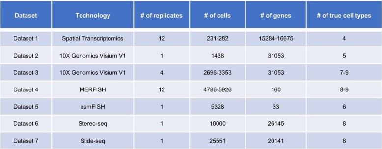
To comprehensively evaluate the performance of different clustering methods, we prepared seven spatial transcriptomics datasets with ground truth information, based on seven real datasets from different technologies. Dataset 1 is based on a mouse olfactory bulb dataset obtained using the spatial transcriptomics technology [20], which measures read counts for pre-determined array spots. This dataset contains 12 mouse brain tissue slices, and we treat each tissue slice as a separate replicate. Dataset 2 is based on a mouse kidney coronal dataset [21] containing a single replicate. Dataset 3 is based on a mouse brain sagittal dataset [22]. As there are two sagittal sections, with each section composed of two cuts (a sagittal-anterior cut and a sagittal-posterior cut), we refer to each cut as a separate replicate. Both Datasets 2 and 3 are based on the 10x Genomics Visium v1 technology [8], which measures read counts for array spots. Dataset 4 is based on a mouse hypothalamic preoptic dataset [23] obtained using the MERFISH technology [24], and the read counts were measured for single cells. We chose animal one for our analysis, which contains 12 different bregma levels (i.e. replicates). Dataset 5 is based on a mouse somatosensory cortex dataset generated using the osmFISH technology [25]. Dataset 6 is based on a mouse olfactory bulb dataset generated using the Stereo-seq technology [26]. Dataset 7 is based on a mouse brain cerebellum dataset obtained from the Slide-seq technology [27]. Both Datasets 5 and 7 have a single-cell resolution. The complete information on dataset size, technology and cell-type number is summarized in Table 1. For Datasets 1–5 and 7, we directly used the spatial locations in the real data; for Dataset 6, we first sampled 10,000 spots from the real data and used the locations of these spots. Then, we generated corresponding simulated read counts and Hematoxylin and Eosin (H&E) stained images as described below (Figure 1).

Table 1.

Summary of the data characteristics. The last column refers to the number of cell types selected using the RShiny program (see Supplementary Methods).

Figure 1.

Simulated H&E-stained images and true cell-type assignments of Datasets 1–7. (A, C, E, G, I, K, M): Simulated H&E-stained images of Datasets 1 to 7. (B, D, F, H, J, L, N): Cells or spots are shown in actual spatial coordinates and colored by their true labels. Datasets are ordered based on increasing number of cells or spots.

Read count matrix

In order to systematically evaluate the performance of different clustering methods, ground truth cell-type labels are needed as a basis to compute quantitative measures. We designed an RShiny program to assign true cell-type labels to individual cells (or spots) in the simulated data, using the spatial locations provided by the real data and accounting for predetermined spatial patterns (see Supplementary Figure S1 and Supplementary Methods). Given each true cell type and corresponding read counts from the real data, we then used scDesign2 [28, 29], a simulator that can generate high-fidelity single-cell gene expression count data and preserve gene–gene correlations, to simulate read counts for synthetic cells. Compared with directly using real counts and corresponding cell-type annotations, the generative model in scDesign2 can help remove noises introduced by mislabeled cells. We compared three gene-wise statistics (the count mean, the count variance and the gene-wise proportion of zero counts) and two cell-wise statistics (the total read count and the cell-wise proportion of zero counts) between simulated and corresponding real data for every dataset, and confirmed that the simulated gene expression captures real-data characteristics (Supplementary Figures S2–S3). We also confirmed that the within-cell-type correlations are indeed larger than between-cell-type correlations (Supplementary Figures S4–S10).

H&E-stained image

H&E is widely used for histology staining and the resulting image is usually characterized by colors ranging from dark purple to pink [30]. As most studies implement spatial transcriptomics methods with histological staining [31], several clustering methods, including SpaCell [17], SpaGCN [16] and stLearn [15], also take the stained images as either an optional or required input to cluster cells (or spots). Since different cell layers or cell types sometimes have distinguishable color patterns, it is valuable to evaluate how these methods perform compared with other methods that do not utilize the histology information. For these methods, we simulated pixel values for red, green and blue (RGB) in a way that reflects the realistic H&E color range and true cell-type assignment (Supplementary Methods).

Clustering methods

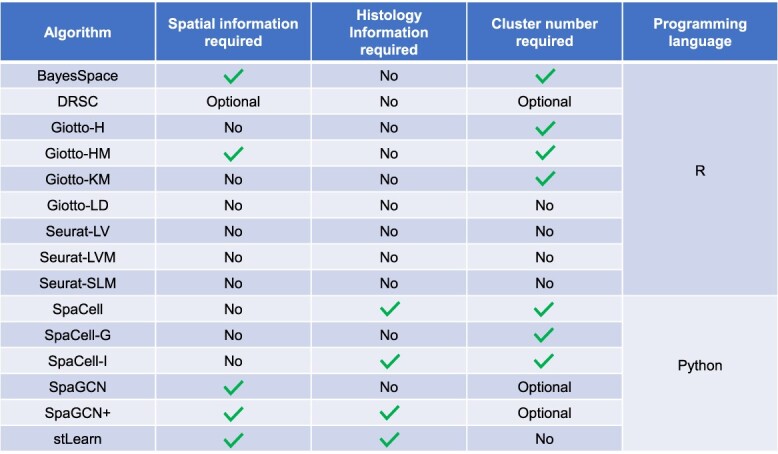
We consider a clustering method as a collection of functions and/or algorithms that take the observed spatial transcriptomics data as the input and output cluster labels. In this study, we compared 15 clustering methods provided by the following seven software tools. A detailed summary of required inputs and programming languages of these methods are summarized in Table 2.

Table 2.

A summary of the 15 clustering methods based on algorithm input and programming language

Seurat [32] is an R toolkit for single-cell genomic data analysis and provides methods for dimensionality reduction and clustering of spatial transcriptomics data. This software includes the option to select multiple clustering methods that only utilize gene expression information. For our analysis, we chose the Louvain (Seurat-LV), Louvain with multi-level refinement (Seurat-LM) and the smart local moving (Seurat-SLM) methods.

The Giotto-Analyzer R toolbox [13] is a specialized package for single-cell spatial transcriptomics analysis. In our comparison, we considered four clustering methods provided by this package: Leiden algorithm (Giotto-LD), Kmeans clustering (Giotto-KM), hierarchical clustering (Giotto-H) and a method based on the hidden Markov random field model (Giotto-HM). Giotto-LD, Giotto-KM and Giotto-H use only gene expression data to perform clustering, while Giotto-HM also uses spatial locations in addition to gene expression information. Additionally, Giotto-HM requires users to input a beta parameter, which defines the strength of the interaction of cells. We set the range of beta parameters as recommended in Giotto’s tutorial (see Supplementary Methods) and selected the results corresponding to the optimal beta value in that range.

The BayesSpace R package implements a Bayesian method with the same name [14]. Using both gene expression and spatial data, the BayesSpace method learns a low-dimensional representation of the gene expression matrix and encourages neighboring spots to belong to the same cluster via a spatial prior.

The DR.SC R package implements a dimensionality reduction and spatial clustering method based on a hidden Markov random field model [18]. The clustering is performed by combining a Gaussian mixture model and a Potts model.

The SpaCell Python package implements a method based on pre-trained convolutional neural networks and autoencoders [17]. Since SpaCell has different options of input data, we use SpaCell to denote the method taking both gene expression and histology data, SpaCell-G to denote the method taking gene expression data alone and SpaCell-I to denote the method taking histology data alone.

The SpaGCN Python package implements a graph convolutional network method with the same name [16]. Using gene expression, spatial locations and histology data (optional), SpaGCN constructs a weighted undirected graph of the spots and carries out the clustering analysis on the constructed graph. Since the histology data are optional, we use SpaGCN to denote the method without using histology information and SpaGCN+ to denote the method with histology data as an input.

The stLearn Python package implements a computational workflow with the same name [15]. Using gene expression, spatial locations and histology data, stLearn performs spatial normalization followed by clustering in a low-dimensional space.

Comparison of clustering accuracy

We applied the 15 methods described in Table 2 to the seven datasets and obtained their inferred cell cluster labels. To quantitatively evaluate and compare the clustering performance, we calculated an adjusted Rand index (ARI) between every set of true cell-type labels and the labels inferred by the clustering methods. For each dataset and method, the performance was summarized using the mean and standard deviation of the ARI score across replicates (Figure 2A–G).

Figure 2.

Comparison of clustering accuracy based on seven spatial transcriptomics datasets. (A–G): Mean adjusted Rand index (ARI) scores for Datasets 1–7. The vertical bars indicate one standard deviation above or below the average score (when more than one replicate is available). (H): Ranking of methods based on average ARI scores. (I): Ranking of methods based on standard deviations of ARIs, for Datasets 1, 3 and 4 which have multiple replicates. Methods with higher average ARI or lower standard deviation are ranked better. Methods are ordered by average ranks in the heatmaps, with methods on the top being the best. The entries marked by NA indicate that the method encountered an error for that dataset.

Even though the Seurat-based methods (Seurat-LV, Seurat-LVM and Seurat-SLM) do not use any spatial or histology information in clustering, they are among the most accurate methods on Datasets 1, 3, 4 and 6. In addition, differences between Seurat-based methods are negligible across all datasets. Three Giotto-based methods (Giotto-H, Giotto-KM Giotto-LD), and SpaCell-G also only use gene expression for clustering, but consistently demonstrate lower accuracy than Seurat-based methods. Since Seurat-based and Giotto-based methods have implemented a series of different clustering algorithms, these results suggest that data processing procedures used by the software may also play an important role in clustering accuracy.

We also compared the four methods that use both gene expression and spatial locations for clustering, including SpaGCN, BayesSpace, Giotto-HM and DRSC. We observed that SpaGCN and BayesSpace perform well on selected datasets, especially when strong spatial patterns are present. For example, BayesSpace is the most accurate on Dataset 2, and SpaGCN is the most accurate on Datasets 3, 5 and 7. However, on Dataset 4, whose spatial distribution of cell types is less obvious, these two methods have lower accuracy than Seurat-based methods. As for the Giotto-HM method, it does not outperform the other Giotto-based methods that do not utilize spatial information. We suspect that Giotto-HM’s heavy reliance on parameter tuning affects its performance on complex data. The DRSC method has an intermediate-level performance on most datasets.

Next, we compared SpaGCN+, stLearn and SpaCell, which incorporate both gene expression and histology information for clustering. On most datasets, stLearn and SpaGCN+ have better performance than SpaCell. stLearn and SpaGCN+ have similar performance on Datasets 5 to 7, but rank very differently on Datasets 1 to 4. Interestingly, SpaGCN+ consistently performs worse than SpaGCN, suggesting that the default configuration of the SpaGCN package does not efficiently leverage histology information to improve performance beyond the use of only gene expression and spatial locations. In addition, we found that stLearn is among the top methods on five datasets, but attains below-average ARIs on Datasets 2 and 3, both of which are based on the 10X Visium technology and sequence the largest number of genes.

We summarized the ranking of each method based on the average ARI scores (Figure 2H) and the standard deviation of ARI across replicates (Figure 2I). Seurat-LVM, SpaGCN, Seurat-LV, Seurat-SLM and stLearn are ranked in the top five by average ARI, which shows that clustering methods using spatial locations and/or histology information did not systematically outperform methods only using gene expression levels. We also compared the concordance between different software packages, but did not observe consistent relationships across datasets (Supplementary Figures S11–S17). In terms of performance across replicates, Seurat-based methods, SpaGCN and stLearn demonstrate better robustness given variation in the data. In summary, Seurat-LVM, SpaGCN and Seurat-LV perform the best and are the most stable across replicates, followed by Seurat-SLM and stLearn.

Comparison of robustness to sequencing depth

Since real datasets often differ in sequencing depths (Supplementary Figure S18), we performed a comparative analysis to evaluate the robustness of different clustering methods given varying sequencing depths. For each dataset in Table 1, we downsampled the read count matrix to a decreasing percentage of the original sequencing depth (from 90% to 10%) (Supplementary Figure S19). The clustering methods were then applied to these new datasets with reduced sequencing depth, and the average ARI score across replicates was used as a summary of performance for every percentage (Figures 3–4).

Figure 3.

Comparison of average clustering accuracy across replicates given a decreasing percentage of original sequencing depth. (A, C, D): Replicates are directly available based on data presented in Table 1. (B, E, F, G): Since the original dataset only has one replicate, for each percentage, five technical replicates were generated in the downsampling process.

Figure 4.

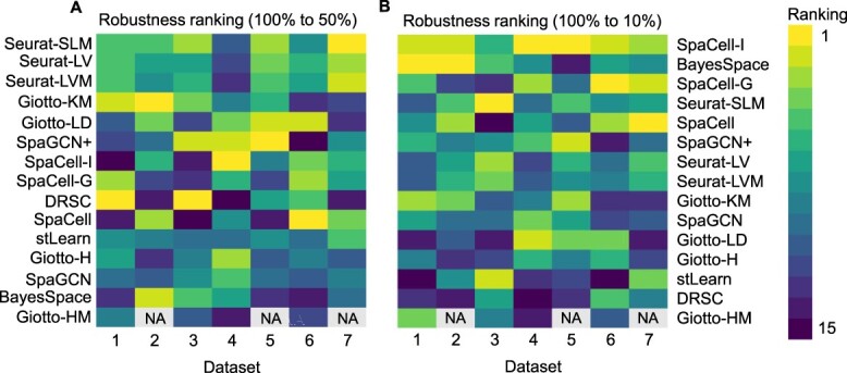
Ranking of methods based on robustness to decreased sequencing depth. Robustness is compared based on the absolute value difference in mean ARI scores when the sequencing depth is reduced to 50% (A) or 10% (B) of the original depth. In both heatmaps, a smaller difference is ranked higher. Entries marked with NA indicate that the corresponding method encountered errors on that dataset.

Among the methods that do not use spatial or histology information, the Seurat-based methods have a more stable performance in average ARI score than do the Giotto-based methods for Datasets 2 and 3, both of which are based on the 10x Genomics Visium technology. However, for all other datasets, the Seurat-based methods have a similar trend to the Giotto-based methods. Even though the SpaCell-G method overall has a smaller change in performance when sequencing depth decreases, its average accuracy is still lower than that of Seurat-based or Giotto-based methods.

We also compared the robustness of methods that use both gene expression and spatial information, namely BayesSpace, Giotto-HM, SpaGCN and DRSC. When the sequencing depth reduces to 50% (Figure 4A), the most robust method among the four is DRSC, followed by Giotto-H, SpaGCN and BayesSpace. However, we observed a reverse order when the sequencing depth reduces to 10% (Figure 4B). In addition, we found that the average ARI scores of BayesSpace and SpaCell-based methods sometimes increase when sequencing depth reduces, for example, in Datasets 2 and 5 (Figure 3B,E). This unexpected performance suggests that these methods may not be efficient enough in distinguishing biological signals and noises. For these methods, the downsampling process helps remove some medium to lowly expressed genes and sometimes improves the signal-to-noise ratio.

Lastly, we compared SpaGCN+, stLearn and SpaCell, which incorporate both gene expression and histology information for clustering. SpaGCN+ and SpaCell have a similar overall performance in robustness to sequencing depth, and both are generally more robust than stLearn.

Comparison of robustness to clustering parameter

The number of true cell types is often unknown to users in practical applications of clustering, but it may have a significant impact on the quality of clustering results. Therefore, we evaluated seven methods for which users are required to input a parameter of cluster number, and three methods for which the parameter is optional (Table 2). For each dataset, we evaluated these methods with different cluster number parameters up to two integer values above or below the ground truth. The average ARI across replicates (Table 1) was then computed to measure clustering performance.

The ARI scores resulting from different cluster number parameters suggest that SpaGCN, SpaGCN+ and BayesSpace generally have more accurate clustering results when the specified cluster number is closer to the true cell-type number (Figure 5A–G). For Datasets 1–3, a sharper decrease in performance is observed when the cluster number parameter is lower than the true cell-type number, compared with cluster parameter being greater than the cell-type number. However, for Dataset 4, which presents a more challenging clustering problem than the other datasets (Figure 2), most methods have improved clustering performance when the cluster number parameter decreases (Figure 5D).

Figure 5.

Comparison of clustering methods based on robustness to clustering parameter. (A–G): Mean ARI of clustering methods given different parameters of cluster number. Change in parameter (the -axis) denotes the difference between the input parameter of cluster number and the true cell type number of a dataset. (H): Ranking of methods according to the mean ARI score across parameter values. Methods with a higher average ARI score across parameter choices are ranked better. Methods are ordered by average ranks across datasets. Entries marked with NA indicate that the method encountered errors on that dataset.

Unlike the methods that utilize spatial information, the Giotto-based methods and SpaCell-based methods do not have a consistent dependence on the cluster number parameter. Moreover, setting the parameter to true cell-type number usually does not lead to the best clustering accuracy of these two types of clustering methods, suggesting the existence of systematic bias. Since the cluster number is often determined based on an estimation of the true cell-type number, we also compared the mean ARI of each method across different parameter values, which suggest SpaGCN, SpaGCN+ and Giotto-H as the best three methods in terms of robustness to the clustering parameter (Figure 5H).

Comparison of robustness to variation in histology images

Histology images often provide useful information to distinguish between different cell populations, so some clustering methods take the histology image as an additional input and attempt to extract distinguishing features for use in the clustering process. In this section, we compare the robustness of SpaGCN+, stLearn, SpaCell and SpaCell-I given histology images with different levels of variation. For each dataset, we simulated five histology images by varying the standard deviations of the pixel colors (Supplementary Methods). A larger standard deviation led to less distinct information about different cell types (Figure 6A and Supplementary Figure S20). Then, we applied the four methods to the same spatial transcriptomics datasets combined with different histology images and compared their clustering accuracy (Figure 6B–H).

Figure 6.

Comparison of clustering methods based on robustness to variation in histology images. (A): Histology images for Dataset 5 that were simulated with an increasing standard deviation. (B–H): Mean ARI of SpaGCN+, SpaCell, SpaCell-I and stLearn given histology images of different levels of variation for Datasets 1–7.

For SpaCell and SpaCell-I, we observed a slight decreasing trend of clustering accuracy when the images have greater variation. In addition, the SpaCell method which uses both gene expression data and histology images consistently has better performance than SpaCell-I, which only uses the images. However, the clustering accuracy of stLearn and SpaGCN+ has a little change on most datasets. Moreover, when these two methods demonstrate obvious changes, they are not guaranteed to have higher accuracy when histology images have a larger signal-to-noise ratio. Since the synthetic histology images were generated with different mean RGB values for different cell types, clustering based on low-variation images supposedly should have better performance than that based on high-variation images, provided that a clustering method can effectively extract and utilize the histology information. However, based on these results, current methods leave room for improvement in their joint analysis of gene expression, spatial and histology information to identify cell populations.

Comparison of software usage

To compare the computational efficiency of different clustering algorithms, we recorded the maximum memory usage and runtime of the methods on Datasets 1–7.

For memory usage, SpaCell-based methods overall use the least memory, followed by SpaGCN-based methods and Seurat-based methods (Figure 7A). The two most memory-demanding methods, BayesSpace and stLearn, both account for spatial locations in their models. As for runtime, Seurat-based methods, SpaGCN-based methods and Giotto-LD have comparable efficiency (Figure 7B). Most methods have a roughly linear trend when dataset size increases from Dataset 1 to Dataset 7. The exception to this trend is Giotto-KM, whose runtime increases significantly.

Figure 7.

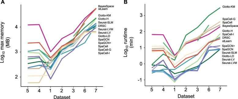
Comparison of clustering methods based on maximum memory usage and runtime. (A): Log of maximum memory measured in megabytes and used by the entire clustering pipeline for each method, including pre-processing. (B): Log of runtime measured in minutes. Datasets are ordered based on cell number gene number. In each panel, methods marked on the right are ordered based on results on Dataset 7. Since Giotto-HM encountered errors on Datasets 2, 5 and 7, its memory usage and runtime are not displayed for these three datasets.

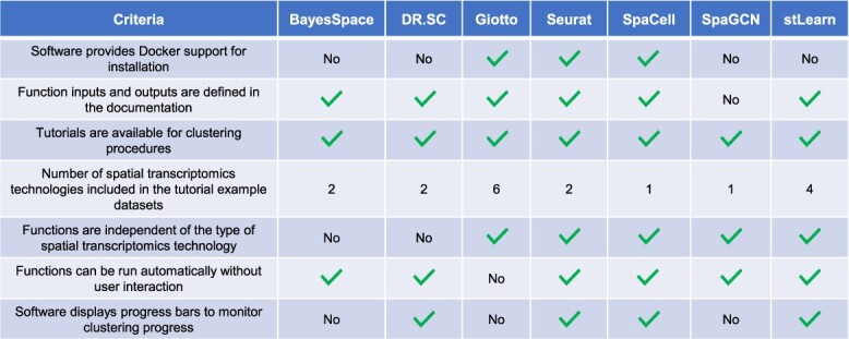
We then compared the software packages for each method based on installation, documentation and usability. The strengths and weaknesses of each software package with respect to these criteria were then summarized in Table 3. Taking all the criteria into consideration, the Seurat, SpaCell and stLearn packages provide better support than the other packages.

Table 3.

Comparison of software packages based on installation, documentation and usability

Comparison based on real data

We performed the majority of comparisons based on the seven semi-synthetic datasets, since gold standard cell-type labels are not yet available for existing spatial transcriptomic datasets. To shed light on method performance on real data, we also compared the clustering accuracy of the 15 methods on five real spatial transcriptomics datasets (Supplementary Table S1), treating cell-type labels reported from the original publications as a reference to evaluate the clustering results. From these results, we found that Seurat-SLM, BayesSpace, Giotto-LD, Giotto-H and SpaGCN have the best clustering accuracy on real datasets 1 to 5, respectively (Supplementary Figure S21). When comparing the relative performance of different methods across datasets, we found that among methods not requiring histology images, Seurat-based methods, BayesSpace and SpaGCN have the best accuracy (Supplementary Figure S22). Furthermore, among methods that depend on histology images as input, SpaGCN+ and stLearn have similar rankings and both outperform the SpaCell-based methods. These results coincide with our observations on the simulated data.

Discussions and Conclusions

In this article, we have benchmarked 15 clustering methods for spatially resolved transcriptomics data based on clustering accuracy, clustering robustness to various sources of variation, computational efficiency and software usability. Our results on seven semi-synthetic datasets highlight the following key findings. First, in terms of clustering accuracy, Seurat-LVM, SpaGCN and Seurat-LV are overall the most accurate clustering methods. However, methods that use additional information from spatial coordinates and histology images do not systematically outperform methods that only use gene expression information. Second, given decreased sequencing depth to 50%, Seurat-based methods are the most robust methods. Again, incorporating spatial or histology information does not guarantee to improve clustering robustness in existing methods. Third, among methods that require users to specify the number of clusters, SpaGCN, SpaGCN+ and Giotto-H maintain the highest average clustering accuracy when given mis-specified parameter values. Fourth, for clustering methods that take histology images as input (stLearn, SpaGCN+, SpaCell and SpaCell-I), they do not demonstrate obvious improvement when images of better quality are supplied. Fifth, Seurat-based and SpaGCN-based methods have the best computational efficiency, and Seurat, SpaCell and stLearn have the best software support. In summary, the additional spatial and histology information provided by spatial transcriptomics data opens new avenues for the development of clustering methods, and we have indeed observed increased accuracy in cell population identification in selected datasets. However, there remain important subjects of future research, including how to more effectively incorporate spatial and histology information in the presence of noises and how to alleviate the dependence of clustering on user-specified cluster numbers or other clustering parameters.

In addition, we would like to discuss two future directions. First, in this study, we utilized semi-synthetic datasets with real spatial locations and synthetic gene expression data generated by the scRNA-seq simulator scDesign2, since real spatial transcriptomics datasets with high-quality cell-type labels are very rare. We anticipate that the comparison can be extended to spatial data with real gene expression levels after curated spatial transcriptomics atlas becomes available. Second, this is a fast evolving field, and we have noticed several new clustering methods during the preparation of this manuscript, including STAGATE [33], SEDR [34], ClusterMap [35] and SC-MEB [36]. To support further comparison of new methods, we have uploaded the data analyzed in this study to a publicly available repository at Github (https://github.com/acheng416/Benchmark-CTCM-ST).

Key Points

• Spatially resolved transcriptomics data provide spatial locations and sometimes histology information in addition to gene expression levels. These additional sources of information are being explored to further improve identification of cell populations.

• Among the 15 clustering methods, we have summarized the best-performing methods in terms of clustering accuracy, clustering robustness to various sources of variation, computational efficiency and software usability.

• Current clustering methods that use spatial location and/or histology information show promising results in selected datasets, but do not consistently perform better and are not more robust to variations in the data than methods that only use gene expression.

• Our comparison indicates that for the clustering of spatial transcriptomics data, there are still opportunities to enhance the overall accuracy and robustness by improving information extraction and feature selection from spatial and histology data.

Data Availability

The mouse olfactory bulb dataset (for Dataset 1 and Real dataset 1 in Table S1) is available from from DOI: 10.1126/SCIENCE.AAF2403. The coronal mouse kidney section (Dataset 2) is available from https://www.10xgenomics.com/resources/datasets. The mouse brain serial sections corresponding to Dataset 3 were obtained from the mouse brain serial section 1 and section 2 datasets at https://www.10xgenomics.com/resources/datasets. The mouse hypothalamic preoptic dataset (for Dataset 4 and Real dataset 4 in Table S1) can be obtained from DOI: 10.5061/dryad.8t8s248. The mouse somatosensory cortex dataset (for Dataset 5 and Real dataset 3 in Table S1) is available from http://linnarssonlab.org/osmFISH/availability/. The Stereo-seq dataset (for Dataset 6 and Real dataset 5 in Table S1) is available from https://db.cngb.org/stomics/mosta/. The mouse brain cerebellum dataset (Dataset 7) is available from https://singlecell.broadinstitute.org/single_cell/study/SCP354. The simulated data generated in this study are available at https://github.com/acheng416/Benchmark-CTCM-ST. Real dataset 2 (Table S1) is available from http://research.libd.org/spatialLIBD/ [37].

Author Biographies

Andrew Cheng is currently pursuing a Master of Science in Computer Science at Stanford University. He is interested in machine learning and bioinformatics.

Guanyu Hu is an assistant professor at the Department of Statistics of the University of Missouri, Columbia, He obtained Ph.D. in Statistics from Florida State University and his research focuses on Bayesian nonparametric methods and sports analytics.

Wei Vivian Li is an assistant professor at the Department of Statistics of the University of California, Riverside. She has a Ph.D. in Statistics and her research focuses on statistical and machine learning methods for biological and biomedical data. Dr. Li was at Rutgers School of Public Health, where part of this work was done.

Funding

This work was supported by National Institutes of Health (NIH) NIGMS R35GM142702, National Science Foundation (NSF) IIS-2128307, Rutgers Busch Biomedical Grant (to W.V.L.), and NSF BCS-2152822, NSF DMS-2210371 (to G.H.).

References

- 1. Larsson L, Frisén J, Lundeberg J. Spatially resolved transcriptomics adds a new dimension to genomics. Nat Methods 2021;18(1):15–8. [DOI] [PubMed] [Google Scholar]
- 2. Dries R, Chen J, Del Rossi N, et al. Advances in spatial transcriptomic data analysis. Genome Res 2021;31(10):1706–18. [DOI] [PMC free article] [PubMed] [Google Scholar]
- 3. Close JL, Long BR, Zeng H. Spatially resolved transcriptomics in neuroscience. Nat Methods 2021;18(1):23–5. [DOI] [PubMed] [Google Scholar]
- 4. Liao J, Xiaoyan L, Shao X, et al. Uncovering an organ’s molecular architecture at single-cell resolution by spatially resolved transcriptomics. Trends Biotechnol 2021;39(1):43–58. [DOI] [PubMed] [Google Scholar]
- 5. Xia C, Fan J, Emanuel G, et al. Spatial transcriptome profiling by merfish reveals subcellular rna compartmentalization and cell cycle-dependent gene expression. Proc Natl Acad Sci 2019;116(39):19490–9. [DOI] [PMC free article] [PubMed] [Google Scholar]
- 6. Codeluppi S, Borm LE, Zeisel A, et al. Spatial organization of the somatosensory cortex revealed by osmfish. Nat Methods 2018;15(11):932–5. [DOI] [PubMed] [Google Scholar]
- 7. Eng C-HL, Lawson M, Zhu Q, et al. Transcriptome-scale super-resolved imaging in tissues by rna seqfish+. Nature 2019;568(7751):235–9. [DOI] [PMC free article] [PubMed] [Google Scholar]
- 8. Ståhl PL, Salmén F, Vickovic S, et al. Visualization and analysis of gene expression in tissue sections by spatial transcriptomics. Science 2016;353(6294):78–82. [DOI] [PubMed] [Google Scholar]
- 9. Rodriques SG, Stickels RR, Goeva A, et al. Slide-seq: A scalable technology for measuring genome-wide expression at high spatial resolution. Science 2019;363(6434):1463–7. [DOI] [PMC free article] [PubMed] [Google Scholar]
- 10. Kiselev VY, Andrews TS, Hemberg M. Challenges in unsupervised clustering of single-cell rna-seq data. Nat Rev Genet 2019;20(5):273–82. [DOI] [PubMed] [Google Scholar]
- 11. Sheng J, Li WV. Selecting gene features for unsupervised analysis of single-cell gene expression data. Brief Bioinform 2021;22(6):bbab295. [DOI] [PMC free article] [PubMed] [Google Scholar]
- 12. Sun S, Zhu J, Zhou X. Statistical analysis of spatial expression patterns for spatially resolved transcriptomic studies. Nat Methods 2020;17(2):193–200. [DOI] [PMC free article] [PubMed] [Google Scholar]
- 13. Dries R, Zhu Q, Dong R, et al. Giotto: a toolbox for integrative analysis and visualization of spatial expression data. Genome Biol 2021;22(78). [DOI] [PMC free article] [PubMed] [Google Scholar]
- 14. Zhao E, Stone MR, Ren X, et al. Spatial transcriptomics at subspot resolution with BayesSpace. Nat Biotechnol 2021;39:1375–84. [DOI] [PMC free article] [PubMed] [Google Scholar]
- 15. Pham D, Tan X, Jun X, et al. stLearn: integrating spatial location, tissue morphology and gene expression to find cell types, cell-cell interactions and spatial trajectories within undissociated tissues. bioRxiv2020. 10.1101/2020.05.31.125658. [DOI]
- 16. Jian H, Li X, Coleman K, et al. SpaGCN: Integrating gene expression, spatial location and histology to identify spatial domains and spatially variable genes by graph convolutional network. Nat Methods 2021;18:1342–51. [DOI] [PubMed] [Google Scholar]
- 17. Tan X, Andrew S, Tran M, et al. Spacell: integrating tissue morphology and spatial gene expression to predict disease cells. Bioinformatics 2019;36(7):2293–4. [DOI] [PubMed] [Google Scholar]
- 18. Wei Liu X, Liao YY, Lin H, et al. Joint dimension reduction and clustering analysis of single-cell rna-seq and spatial transcriptomics data. Nucleic Acids Res 2022;50(12):e72–2. [DOI] [PMC free article] [PubMed] [Google Scholar]
- 19. Rao A, Barkley D, França GS, et al. Exploring tissue architecture using spatial transcriptomics. Nature 2021;596(7871):211–20. [DOI] [PMC free article] [PubMed] [Google Scholar]
- 20. Ståhl PL, Salmén F, Vickovic S, et al.. Visualization and analysis of gene expression in tissue sections by spatial transcriptomics. Science 2016; 353(6294): 78–82. [DOI] [PubMed] [Google Scholar]
- 21. Mouse Kidney Section from C57BL/6 mice (Visium Demonstration v1 Chemistry) . Spatial Gene Expression Dataset by Space Ranger 1.1.0, 10x Genomics, 2020.
- 22. Mouse Brain Serial Sections from C57BL/6 mice (Visium Demonstration v1 Chemistry) . Spatial Gene Expression Dataset by Space Ranger 1.1.0, 10x Genomics, 2020.
- 23. Moffitt JR, Bambah-Mukku D, Eichhorn SW, et al. Molecular, spatial, and functional single-cell profiling of the hypothalamic preoptic region. Science 2018;362(6416):eaau5324. [DOI] [PMC free article] [PubMed] [Google Scholar]
- 24. Chen KH, Boettiger AN, Moffitt JR, et al. Spatially resolved, highly multiplexed RNA profiling in single cells. Science 2015;348(6233). [DOI] [PMC free article] [PubMed] [Google Scholar]
- 25. Codeluppi S, Borm LE, Zeisel A, et al.. Spatial organization of the somatosensory cortex revealed by osmFISH. Nat Methods 2018; 15:932–5. [DOI] [PubMed] [Google Scholar]
- 26. Chen A, Liao S, Cheng M, et al. Spatiotemporal transcriptomic atlas of mouse organogenesis using dna nanoball-patterned arrays. Cell 2022;185(10):1777–92. [DOI] [PubMed] [Google Scholar]
- 27. Rodriques SG, Stickels RR, Goeva A, et al. Slide-seq: A scalable technology for measuring genome-wide expression at high spatial resolution. Science 2019; 363(6434): 1463–7. [DOI] [PMC free article] [PubMed] [Google Scholar]
- 28. Sun T, Song D, Li WV, et al. scDesign2: a transparent simulator that generates high-fidelity single-cell gene expression count data with gene correlations captured. Genome Biol 2021;22(163). [DOI] [PMC free article] [PubMed] [Google Scholar]
- 29. Li WV, Li JJ. A statistical simulator scdesign for rational scrna-seq experimental design. Bioinformatics 2019;35(14):i41–50. [DOI] [PMC free article] [PubMed] [Google Scholar]
- 30. Chan JKC. The wonderful colors of the hematoxylin–eosin stain in diagnostic surgical pathology. Int J Surg Pathol 2014;22(1):12–32. [DOI] [PubMed] [Google Scholar]
- 31. Longo SK, Guo MG, Ji AL, et al. Integrating single-cell and spatial transcriptomics to elucidate intercellular tissue dynamics. Nat Rev Genet 2021;1–18. [DOI] [PMC free article] [PubMed] [Google Scholar]
- 32. Satija R, Farrell JA, Gennert D, et al. Spatial reconstruction of single-cell gene expression data. Nat Biotechnol 2015;33:495–502. [DOI] [PMC free article] [PubMed] [Google Scholar]
- 33. Dong K, Zhang S. Deciphering spatial domains from spatially resolved transcriptomics with an adaptive graph attention auto-encoder. Nat Commun 2022;13(1):1–12. [DOI] [PMC free article] [PubMed] [Google Scholar]
- 34. Huazhu F, Hang X, Chong K, et al. Unsupervised spatially embedded deep representation of spatial transcriptomics. Biorxiv 2021. [DOI] [PMC free article] [PubMed] [Google Scholar]
- 35. He Y, Tang X, Huang J, et al. Clustermap for multi-scale clustering analysis of spatial gene expression. Nat Commun 2021;12(1):1–13. [DOI] [PMC free article] [PubMed] [Google Scholar]
- 36. Yang Y, Shi X, Liu W, et al. Sc-meb: spatial clustering with hidden markov random field using empirical bayes. Brief Bioinform 2022;23(1):bbab466. [DOI] [PMC free article] [PubMed] [Google Scholar]
- 37. Pardo B, Spangler A, Weber LM, et al. spatiallibd: an r/bioconductor package to visualize spatially-resolved transcriptomics data. BMC Genomics 2022;23(1):1–5. [DOI] [PMC free article] [PubMed] [Google Scholar]
Associated Data
This section collects any data citations, data availability statements, or supplementary materials included in this article.
Supplementary Materials
Data Availability Statement