Learning continuous potentials from smFRET

Abstract

Potential energy landscapes are useful models in describing events such as protein folding and binding. While single-molecule fluorescence resonance energy transfer (smFRET) experiments encode information on continuous potentials for the system probed, including rarely visited barriers between putative potential minima, this information is rarely decoded from the data. This is because existing analysis methods often model smFRET output assuming, from the onset, that the system probed evolves in a discretized state space to be analyzed within a hidden Markov model (HMM) paradigm. By contrast, here, we infer continuous potentials from smFRET data without discretely approximating the state space. We do so by operating within a Bayesian nonparametric paradigm by placing priors on the family of all possible potential curves. As our inference accounts for a number of required experimental features raising computational cost (such as incorporating discrete photon shot noise), the framework leverages a structured-kernel-interpolation Gaussian process prior to help curtail computational cost. We show that our structured-kernel-interpolation priors for potential energy reconstruction from smFRET analysis accurately infers the potential energy landscape from a smFRET binding experiment. We then illustrate advantages of structured-kernel-interpolation priors for potential energy reconstruction from smFRET over standard HMM approaches by providing information, such as barrier heights and friction coefficients, that is otherwise inaccessible to HMMs.

Significance

We introduce structured-kernel-interpolation priors for potential energy reconstruction from single-molecule fluorescence resonance energy transfer data, a tool for inferring continuous potential energy landscapes, including barrier heights and friction coefficients, from single-molecule fluorescence resonance energy transfer data. We benchmark on synthetic and experimental data.

Introduction

Potential energy landscapes are useful continuous space model reductions employed across biophysics (1,2,3,4,5,6). For example, potentials can model dynamics along smooth reaction coordinates (3, 7,8,9,10), including the celebrated protein folding funnel (3,8,11). They also provide a natural language from which to calculate thermodynamic quantities (12,13,14). Furthermore, shapes of landscapes, including barrier heights and friction coefficients, can provide insight into molecular function (15,16), such as molecular motor dynamics (16). As such, inferring accurate potentials is a crucial step toward gaining insight into biophysical systems.

One way by which to decode potential energy landscapes from biological systems is through single-molecule fluorescence resonance energy transfer (smFRET) experiments (17,18,19,20,21). Most commonly, smFRET works by tagging two locations of a biomolecule with pairs of fluorophores. When in proximity, the fluorophore excited by the laser (the donor) may transfer its excitation, via dipole-dipole coupling, over to the acceptor fluorophore (22). As the distance between the donor and acceptor fluorophores change, so too does the efficiency of dipole-dipole energy transfer, resulting in higher donor emission rates when fluorophores are further apart. Conversely, more photons are emitted from the acceptor when fluorophores are in close proximity (22). As such, it is common to use the proportion of donor and acceptor photons counted in a given time window, the FRET efficiency, to estimate the pair fluorophore distance (17,23).

To deduce energies from smFRET data, it is common to immediately assume a discrete state space and invoke hidden Markov models (HMMs) in the ensuing analysis 24,25,26,27,28). HMMs work by partitioning the observed smFRET efficiencies into discrete levels coinciding with distinct states. One can then use smFRET data to infer the number of states in addition to the associated transition rate parameters and pair distances (2,27), which in turn can be used to infer the potential energy of the states using the Boltzmann distribution (2,29).

The above approach is useful in gaining quantitative insight into systems well approximated by discrete states (10,25,26,28). However, the above formulation is not appropriate when the dynamics occur along a continuous reaction coordinate poorly approximated by well-separated discrete states (5,11).

Furthermore, while HMMs can be used to infer each state’s relative energies (though parametric HMMs require a specification in the number of states (30)), they cannot reveal energy barriers between states without preexisting knowledge of internal system parameters, such as the landscape curvature and internal friction, due to loss of information inherent to the discretization process (2,31). The inability to infer accurate potential energy barriers from a single data set without the knowledge of hidden internal parameters is an important limitation of HMMs applied to smFRET data. Furthermore, as we will see shortly, analyzing a continuous system with discrete states may introduce important biases in the expected distances defining the FRET states.

As such, a method capable of inferring potential energy landscapes, including barrier heights and friction coefficients, along a continuous coordinate would greatly enhance the resolution with which we can probe biophysical systems and lend deeper insight into protein folding (11), protein binding (3), and the physics of molecular motors (16).

Here, we develop a method to decode a continuous potential from smFRET data without resorting to discrete state-space assumptions inherent to HMM modeling. We do so by incorporating a detailed, physics-informed likelihood distribution describing the relationship between measurements and a potential energy landscape. We then infer the most probable potential energy landscape within the Bayesian nonparametric paradigm by placing a prior on the potential energy landscape with support over the family of all putative continuous curves. Our prior distribution is built upon the structured-kernel-interpolation Gaussian process (32), which allows for inference of continuous potentials while simultaneously avoiding the costly cubic scaling of conventional Gaussian process regression. Cubic scaling becomes especially problematic as we insist on incorporating realistic measurement features into our likelihood.

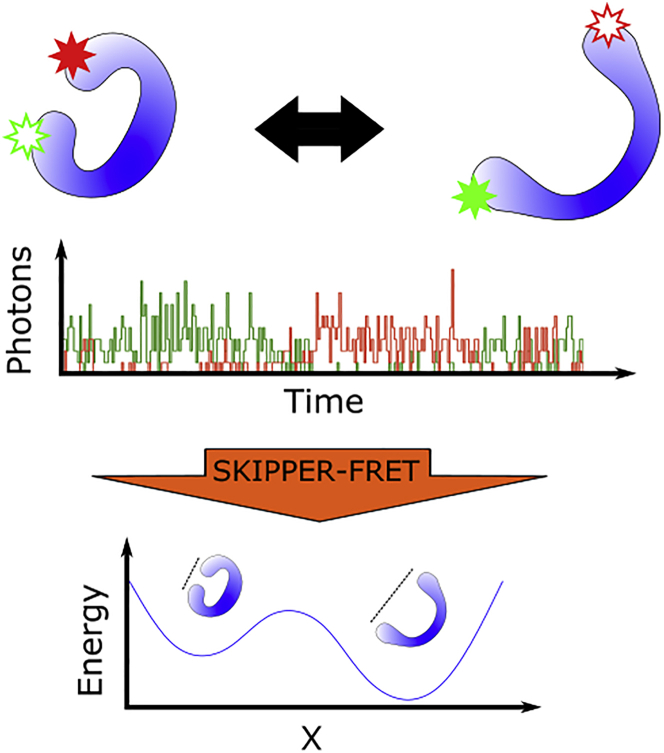
We show that our structured-kernel-interpolation priors for potential energy reconstruction from smFRET (SKIPPER-FRET) analysis unveils the full potential energy landscape, including barrier heights and friction coefficients within reasonable computational times. The essence of SKIPPER-FRET is described in cartoon form in Fig. 1. We benchmark SKIPPER-FRET on synthetic/simulated data as well as experimental data.

Figure 1.

Cartoon description of SKIPPER-FRET. At the top, we see a protein switching between two conformations over time. The protein is labeled with donor and acceptor fluorophores. As the protein changes configuration, the FRET efficiency between the fluorophores also changes. In the middle panel, we illustrate a typical trace containing the number of red and green photons over time. In the bottom panel, we show the outcome of SKIPPER-FRET analysis used to infer the potential energy landscape along the reaction coordinate probed. To see this figure in color, go online.

Materials and methods

Our goal is to learn potentials given photon arrival data from two channels assuming continuous illumination smFRET data. Generalization to pulsed data is possible and addressed in the data acquisition. In this section, we present a forward model describing how a potential gives rise to the data we collect. Next, we describe an inverse model allowing us to infer the potential directly from the data, along with a numerical algorithm developed to sample from our high-dimensional posterior. We conclude by summarizing the experiment we use to validate our method.

Forward model

In our framework, we imagine placing donor and acceptor fluorophores at two points whose relative distance varies with time. That is, we envision either monitoring a molecule undergoing configurational changes along a reaction coordinate or a pair of molecules binding and unbinding; in either case, our formulation is identical. The dynamics of the probes with respect to each other are dictated by a potential we wish to deduce. The labeled system is exposed to continuous illumination in which both fluorophores will be excited. Donor excitations have a position-dependent probability of FRET transfer, whereas acceptor excitations are treated as a source of background. We describe this process in detail in this section.

Pair distance

We begin by assuming that the distance of interest evolves according to Langevin dynamics (5,29)

$$\zeta \frac{dx}{dt}=f\left(x\right)+r\left(t\right)$$ (1)

with unknown constant $\zeta$ (the friction coefficient) and unknown spatially dependent force $\left(f=-\nabla U\right)$. In the above, $r\left(t\right)$ is the thermal noise whose moments read

$$⟨r\left(t\right)⟩=0\mathrm{a}\mathrm{n}\mathrm{d}$$ (2)

$$⟨r\left(t\right)r\left(t^{\prime }\right)⟩=2\zeta kT\delta \left(t-t^{\prime }\right)\text{.}$$ (3)

Here, $kT$ is the usual thermal energy, and $⟨\dots ⟩$ denotes an average over thermal noise realizations. Note that our model assumes a constant friction coefficient.

Under the Ito approximation (33), we can evaluate Eq. 1 on a fine grid of time levels,

$$\frac{\zeta }{\Delta t}\left(x_{n+1}-x_n\right)=f\left(x_n\right)+\sqrt{\frac{2\zeta kT}{\Delta t}}{ϵ}_n\text{,}$$ (4)

where $x_n$ is the distance at time level $n$, $\Delta t$ is the time step size, and ${ϵ}_n$ is a normally distributed random variable with mean 0 and variance 1. We can rewrite the probability of $x_{n+1}$ as follows:

$$\mathcal{P}\left(x_{n+1}|x_n,\zeta ,U\right)=\mathbf{N}\mathbf{o}\mathbf{r}\mathbf{m}\mathbf{a}\mathbf{l}\left(x_{n+1};x_n+\frac{\Delta t}{\zeta }f\left(x_n\right),\frac{2\Delta tkT}{\zeta }\right)\text{,}$$ (5)

which reads “the probability of $x_{n+1}$ given $\zeta$, $U$, and the previous position $\left(x_n\right)$ is a normal distribution with mean $x_n+\frac{\Delta t}{\zeta }f\left(x_n\right)$ and variance $\frac{2\Delta tkT}{\zeta }$”. Here, we let $N$ be the number of time levels and let ${\mathit{x}}_{1:N}$ represent the set of all positions at those time levels. Note that the time step, $\Delta t$, must be chosen to be small enough that the Ito approximation be valid but, in principle, need not coincide with the measurement time scale.

Another important note is in order. When analyzing data from binding experiments, we envision a donor-tagged immobilized biomolecule interacting with an acceptor-tagged binding agent. In this setup, we interpret the pair distance, $x$, as the distance between the donor fluorophore and the nearest acceptor fluorophore with the understanding that the identity of the acceptor fluorophore may change over time.

Photon measurements

To model photon counts, we make a number of physically reasonable assumptions. First, we assume that timescales over which pair distances vary are much slower than fluorophore excited-state relaxation times (23) (microseconds or slower versus nanoseconds (2,10)). Secondly, we assume that the small absorption cross section of the fluorophores results in a low excitation rate compared with the relaxation rate. Thus, the interphoton arrival time is dominated by the excitation rate, ${\lambda }_X$ (23).

As the pair distance is assumed to remain constant over the whole time step (see Eq. 5), the FRET rate will also be assumed constant (with changes approximated as occurring when time levels change). Thus, photon arrival times and the order of photon colors within a time step provide no additional information. In this regime, the probability of the number of measured green, $g_n$, and red, $r_n$, photons are drawn from a Poisson distribution (see supplemental information section S0.5):

$$\mathcal{P}\left(g_n\right)=\mathbf{P}\mathbf{o}\mathbf{i}\mathbf{s}\mathbf{s}\mathbf{o}\mathbf{n}\left(g_n;\Delta t{D}_g\left({\lambda }_X{f}_g\left(x_n\right)+{\lambda }_g\right)\right)\mathrm{a}\mathrm{n}\mathrm{d}$$ (6)

$$\mathcal{P}\left(r_n\right)=\mathbf{P}\mathbf{o}\mathbf{i}\mathbf{s}\mathbf{s}\mathbf{o}\mathbf{n}\left(r_n;\Delta t{D}_r\left({\lambda }_X{f}_r\left(x_n\right)+{\lambda }_r\right)\right)\text{,}$$ (7)

where ${\lambda }_X$ is the donor excitation rate; ${\lambda }_g$ is the green photon background rate; ${\lambda }_r$ is the red photon background rate (which includes the direct acceptor excitation rate); $D_g$ and $D_r$ are detector efficiencies; and $f_g\left(x_n\right)$ and $f_r\left(x_n\right)$ are the fractions of photons emitted by the FRET pair detected in the green and red channels, respectively, calculated from the FRET efficiency as a function of position, $\text{FRET}\left(x\right)$. The cross talk matrix, which encodes the efficiency at which a red photon is measured to be green, and vice versa, reads as follows:

$$\text{FRET}\left(x\right)=\frac{1}{1+{\left(\frac{x}{R_0}\right)}^6}\mathrm{a}\mathrm{n}\mathrm{d}$$ (8)

$$\left[\begin{array}{c}{f}_g\left(x\right)\\ f_r\left(x\right)\end{array}\right]=\left[\begin{array}{cc}{C}_{gg}& C_{gr}\\ C_{rg}& C_{rr}\end{array}\right]\left[\begin{array}{c}1-\text{FRET}\left(x\right)\\ \text{FRET}\left(x\right)\end{array}\right]\text{,}$$ (9)

where $R_0$ is the characteristic distance for the acceptor donor pair at which the FRET efficiency is 0.5 and $C_{ij}$ is the probability that a photon with color $i$ is detected by detector $j$. For example, $C_{rg}$ is the probability that a red photon is detected by the green photon detector.

Inverse model

Our goal is the create a probability distribution for the potential energy landscape, $U\left(x\right)$, the pair distance trajectory, ${\mathit{x}}_{1:N}$, the excitation rate, ${\lambda }_X$, the background photon rates, ${\lambda }_r$ and ${\lambda }_g$, and the friction coefficient, $\zeta$, given a series of photon measurements, ${\mathit{g}}_{1:N}$ and ${\mathit{r}}_{1:N}$. Note that detector efficiencies, $D_g$ and $D_r$, and the cross talk matrix can be calibrated separately and therefore do not need to be inferred. Using Bayes’ theorem, write

$$\mathcal{P}\left(U,{\mathit{x}}_{1:N},{\lambda }_X,{\lambda }_g,{\lambda }_r,\zeta |{\mathit{g}}_{1:N},{\mathit{r}}_{1:N}\right)\propto \mathcal{P}\left({\mathit{g}}_{1:N},{\mathit{r}}_{1:N}|U,{\mathit{x}}_{1:N},{\lambda }_X,{\lambda }_g,{\lambda }_r,\zeta \right)\mathcal{P}\left(U,{\mathit{x}}_{1:N},{\lambda }_X,{\lambda }_g,{\lambda }_r,\zeta \right)\text{.}$$ (10)

The first term on the right side of Eq. 10 is called the likelihood and is equal to the product of Eqs. 6 and 7 for each time level. The second term is called the prior and can further be decomposed as follows

$$\mathcal{P}\left(U,{\mathit{x}}_{1:N},{\lambda }_X,{\lambda }_g,{\lambda }_r,\zeta \right)=\left(\prod _{n=2}^N\mathcal{P}\left(x_n|x_{n-1}U,\zeta \right)\right)\mathcal{P}\left(x_1\right)\mathcal{P}\left(U\right)\mathcal{P}\left(\zeta \right)\mathcal{P}\left({\lambda }_X\right)\mathcal{P}\left({\lambda }_g\right)\mathcal{P}\left({\lambda }_r\right)\text{.}$$ (11)

The first term on the right-hand side, $\mathcal{P}\left(x_n|x_{n-1},U,\zeta \right)$, is the discretized Langevin equation (3.3) (Equation 5). We are free to choose the remaining priors over $\mathcal{P}\left(x_1\right)$, $\mathcal{P}\left(U\right)$, $\mathcal{P}\left(\zeta \right)$, $\mathcal{P}\left({\lambda }_X\right)$, $\mathcal{P}\left({\lambda }_g\right)$, and $\mathcal{P}\left({\lambda }_r\right)$.

We start by placing priors on our photon rates and friction coefficient. We know that our excitation rate, ${\lambda }_X$, is strictly positive, and as such, an acceptable choice of prior is the gamma distribution, which has nonzero probability density along the positive real line

$$\mathcal{P}\left({\lambda }_X\right)=\mathbf{G}\mathbf{a}\mathbf{m}\mathbf{m}\mathbf{a}\left({\lambda }_X;{\kappa }_{{\lambda }_X},{\theta }_{{\lambda }_X}\right)\text{,}$$ (12)

where ${\kappa }_{{\lambda }_X}=2$ is chosen to make the mode of the distribution diffuse (i.e., create an uninformative prior) and ${\theta }_{{\lambda }_X}$ is chosen so as to give a mean expected value close to the average number of observed photons per frame. Similarly, we set a gamma prior on our background photon rates

$$\mathcal{P}\left({\lambda }_r\right)=\mathbf{G}\mathbf{a}\mathbf{m}\mathbf{m}\mathbf{a}\left({\lambda }_r;{\kappa }_{prior:{\lambda }_r},{\theta }_{{\lambda }_r}\right)\mathrm{a}\mathrm{n}\mathrm{d}$$ (13)

$$\mathcal{P}\left({\lambda }_g\right)=\mathbf{G}\mathbf{a}\mathbf{m}\mathbf{m}\mathbf{a}\left({\lambda }_g;{\kappa }_{prior:{\lambda }_g},{\theta }_{{\lambda }_g}\right)\text{,}$$ (14)

where we again choose ${\kappa }_{{\lambda }_r}={\kappa }_{{\lambda }_g}=2$ and choose values for ${\theta }_{{\lambda }_r}$ and ${\theta }_{{\lambda }_g}$ that give mean values close to the measured background rates. Similarly, because $\zeta$ is strictly positive, the gamma distribution is also a good choice. As a prior over the friction coefficient, we choose

$$\mathcal{P}\left(\zeta \right)=\mathbf{G}\mathbf{a}\mathbf{m}\mathbf{m}\mathbf{a}\left(\zeta ;{\kappa }_{\zeta },{\theta }_{\zeta }\right)\text{,}$$ (15)

where ${\kappa }_{\zeta }=2$ and ${\theta }_{\zeta }=\mathrm{5,000}$ ag/ns are chosen to be minimally informative. In other words, we choose ${\kappa }_{\zeta }$ and ${\theta }_{\zeta }$ such that our prior is broad over a physically motivated region (3.4). Note that ${\kappa }_{{\lambda }_X}$, ${\theta }_{{\lambda }_X}$, ${\kappa }_{{\lambda }_g}$, ${\theta }_{{\lambda }_g}$, ${\kappa }_{{\lambda }_r}$, ${\theta }_{{\lambda }_r}$, ${\kappa }_{{\lambda }_{\zeta }}$, and ${\theta }_{{\lambda }_{\zeta }}$ are hyperparameters whose exact values bear little weight on the final form of the posterior as more data are acquired (24)

Next, we place a prior on our initial position. That is, under our dynamics model, Eq. 5, all positions, ${\mathbf{x}}_{2:N}$, are directly conditioned on the previous position, i.e., the dynamics follow a Markov chain. As such, we must only place a prior on the position at the first time level, $x_1$. For computational reasons alone, we choose a normal distribution as the prior over $x_1$ as it matches the form of the transition probability of Eq. 5,

$$\mathcal{P}\left(x_1\right)=\mathbf{N}\mathbf{o}\mathbf{r}\mathbf{m}\mathbf{a}\mathbf{l}\left(x_1;R_0,R_0^2\right)\text{.}$$ (16)

As the initial position is known to be around the characteristic FRET distance up to some uncertainty, we conveniently choose to center our distribution at $R_0$ with standard deviation $R_0$. The latter choices are immaterial in the presence of sufficient data.

Of greatest importance is our choice of prior on potential energy landscape, $U\left(x\right)$. One natural prior choice is the Gaussian process (32,34,35) allowing us to sample from all putative curves without prespecifying any functional form. However, a naive implementation of the Gaussian process is computationally intractable for large data sets as computational complexity scales cubically with the size of the data (32,36). This is especially challenging given the lack of conjugacy between the likelihood and prior rendering direct sampling of the posterior infeasible.

Instead, we develop a computationally efficient adaptation of the Gaussian process, leveraging recent advances in structured-kernel-interpolation Gaussian processes (SKI-GPs) (32,34). Briefly, SKI-GPs work by selecting a set of $M$ nodes, ${\mathbf{x}}_{1:M}^{\ast }$, termed inducing points, where we wish to exactly evaluate the potential. The value of the potential at the inducing points is itself drawn from a zero mean multivariate Normal distribution with some prespecified covariance matrix

$$\mathcal{P}\left({\mathit{U}}_{1:M}^{\ast }\right)=\mathbf{N}\mathbf{o}\mathbf{r}\mathbf{m}\mathbf{a}\mathbf{l}\left({\mathit{U}}_{1:M}^{\ast };\mathbf{0},\mathit{K}\right)$$ (17)

where $\mathit{K}$ is our kernel matrix with elements $K_{ij}=k\left(x_i^{\ast },x_j^{\ast }\right)$, where $k$ is our kernel function defined by

$$k\left(x,y\right)=h^2\exp \left(-\frac{{\left(x-y\right)}^2}{2{\mathcal{l}}^2}\right)\text{,}$$ (18)

where $h$ and $\mathcal{l}$ are hyperparameters setting the prior uncertainty and length scale, respectively, and $x$ and $y$ are two arbitrary arguments. We then interpolate the value of the potential elsewhere (34). For example, collecting the force evaluated along the trajectory into a vector, ${\mathit{f}}_{1:N}$, and the potential evaluated at the inducing points into a vector, ${\mathit{U}}_{1:M}^{\ast }$, we can interpolate

$${\mathit{f}}_{1:N}={\mathit{K}}^{\ast }{\mathit{K}}^{-1}{\mathit{U}}_{1:M}^{\ast }\text{,}$$ (19)

where ${\mathit{K}}^{\ast }$, with elements $K_{nm}^{\ast }=-\nabla k\left(x_n,x_m^{\ast }\right)$, is the kernel matrix between the force at each point in the trajectory and the potential at the inducing points.

Putting together all distributions and priors of our model, we attain a posterior for SKIPPER-FRET given by

$$\mathcal{P}\left({\mathit{U}}_{1:M}^{\ast },{\mathit{x}}_{1:N},\zeta ,{\lambda }_X,{\lambda }_g,{\lambda }_r|{\mathit{r}}_{1:N},{\mathit{g}}_{1:N}\right)\propto \mathbf{N}\mathbf{o}\mathbf{r}\mathbf{m}\mathbf{a}\mathbf{l}\left({\mathit{U}}_{1:M}^{\ast };\mathbf{0},K\right)\mathbf{G}\mathbf{a}\mathbf{m}\mathbf{m}\mathbf{a}\left(\zeta ;{\kappa }_{\zeta },{\theta }_{\zeta }\right)\times \mathbf{G}\mathbf{a}\mathbf{m}\mathbf{m}\mathbf{a}\left({\lambda }_X;{\kappa }_{{\lambda }_X},{\theta }_{{\lambda }_X}\right)\mathbf{G}\mathbf{a}\mathbf{m}\mathbf{m}\mathbf{a}\left({\lambda }_r;{\kappa }_{{\lambda }_r},{\theta }_{{\lambda }_r}\right)\mathbf{G}\mathbf{a}\mathbf{m}\mathbf{m}\mathbf{a}\left({\lambda }_g;{\kappa }_{{\lambda }_g},{\theta }_{{\lambda }_g}\right)\times \mathbf{N}\mathbf{o}\mathbf{r}\mathbf{m}\mathbf{a}\mathbf{l}\left(x_1;R_0,R_0^2\right)\prod _{n=1}^{N-1}\mathbf{N}\mathbf{o}\mathbf{r}\mathbf{m}\mathbf{a}\mathbf{l}\left(x_{n+1};x_n+\frac{\Delta t}{\zeta }f\left(x_n\right),\frac{2\Delta tkT}{\zeta }\right)\times \prod _{n=1}^N\mathbf{P}\mathbf{o}\mathbf{i}\mathbf{s}\mathbf{s}\mathbf{o}\mathbf{n}\left(g_n;\Delta t{D}_g\left({\lambda }_X{f}_g\left(x_n\right)+{\lambda }_g\right)\right)\mathbf{P}\mathbf{o}\mathbf{i}\mathbf{s}\mathbf{s}\mathbf{o}\mathbf{n}\left(r_n;\Delta t{D}_r\left({\lambda }_X{f}_r\left(x_n\right)+{\lambda }_r\right)\right)\text{.}$$ (20)

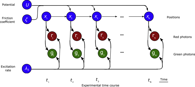
A graphical model of our full posterior, illustrating the conditional dependence of all variables, is shown in Fig. 2.

Figure 2.

Graphical description of the model. Nodes (circles) represent random variables of our model, while arrows connecting the nodes highlight conditional dependency. Blue nodes represent variables we wish to learn in our inference scheme, and the red and green nodes represent the measured photon counts for each bin. To see this figure in color, go online.

Algorithm

Our inverse model leaves us with a high-dimensional posterior, Eq. 20, which does not attain an analytical form and cannot be directly sampled. Thus, we propose using an overall Gibbs sampling (24) scheme to draw samples from our posterior.

Briefly, Gibbs sampling works by starting from an initial guess for the parameters, then iteratively sampling each variable while holding other variables fixed. This scheme, where superscripts indicate the iteration index, is outlined below:

• •Step 1: start with an initial guess for each variable: ${\mathit{U}}_{1:M}^{\ast \left(0\right)}$, ${\mathit{x}}_{1:N}^{\left(0\right)}$, ${\zeta }^{\left(0\right)}$, ${\lambda }_X^{\left(0\right)}$, ${\lambda }_g^{\left(0\right)}$, and 0${\lambda }_r^{\left(0\right)}$.
• •Step 2: for many iterations $i$,

– sample ${\mathit{U}}_{1:M}^{\ast \left(i+1\right)}$ from $\mathcal{P}\left({\mathit{U}}_{1:M}^{\ast }|{\mathit{x}}_{1:N}^{\left(i\right)},{\zeta }^{\left(i\right)},{\lambda }_X^{\left(i\right)},{\lambda }_g^{\left(i\right)},{\lambda }_r^{\left(i\right)},{\mathit{r}}_{1:N},{\mathit{g}}_{1:N}\right)$,

– sample ${\mathit{x}}_{1:N}^{\left(i+1\right)}$ from $\mathcal{P}\left({\mathbf{x}}_{1:N}|{\mathit{U}}_{1:M}^{\ast \left(i+1\right)},{\zeta }^{\left(i\right)},{\lambda }_X^{\left(i\right)},{\lambda }_g^{\left(i\right)},{\lambda }_r^{\left(i\right)},{\mathit{r}}_{1:N},{\mathit{g}}_{1:N}\right)$,

– sample ${\zeta }^{\left(i+1\right)}$ from $\mathcal{P}\left(\zeta |{\mathit{U}}_{1:M}^{\ast \left(i+1\right)},{\mathit{x}}_{1:N}^{\left(i+1\right)},{\lambda }_X^{\left(i\right)},{\lambda }_g^{\left(i\right)},{\lambda }_r^{\left(i\right)},{\mathit{r}}_{1:N},{\mathit{g}}_{1:N}\right)$,

– sample ${\lambda }_X^{\left(i+1\right)}$ from $\mathcal{P}\left({\lambda }_X|{\mathit{U}}_{1:M}^{\ast \left(i+1\right)},{\mathit{x}}_{1:N}^{\left(i+1\right)},{\zeta }^{\left(i+1\right)},{\lambda }_g^{\left(i\right)},{\lambda }_r^{\left(i\right)},{\mathit{r}}_{1:N},{\mathit{g}}_{1:N}\right)$,

– sample ${\lambda }_g^{\left(i+1\right)}$ from $\mathcal{P}\left({\lambda }_g|{\mathit{U}}_{1:M}^{\ast \left(i+1\right)},{\mathit{x}}_{1:N}^{\left(i+1\right)},{\zeta }^{\left(i+1\right)},{\lambda }_X^{\left(i+1\right)},{\lambda }_r^{\left(i\right)},{\mathit{r}}_{1:N},{\mathit{g}}_{1:N}\right)$, and

– sample ${\lambda }_r^{\left(i+1\right)}$ from $\mathcal{P}\left({\lambda }_r|{\mathit{U}}_{1:M}^{\ast \left(i+1\right)},{\mathit{x}}_{1:N}^{\left(i+1\right)},{\zeta }^{\left(i+1\right)},{\lambda }_X^{\left(i+1\right)},{\lambda }_g^{\left(i+1\right)},{\mathit{r}}_{1:N},{\mathit{g}}_{1:N}\right)$.

The conditional probabilities appearing in step 2 above are derived in supporting material section S0.6. Once sufficient samples have been generated (after burn in is discarded (24)), we can use the sample average to provide point estimates for each variable or plot the distribution of all samples drawn.

Data acquisition

We analyze single-photon smFRET data taken from an experiment probing the binding between the nuclear-coactivator binding domain (NCBD) of the CBP/p300 transcription factor and the activation domain of SRC-3 (ACTR) (37). ACTR and NCBD are both intrinsically disordered proteins (37,38,39). In the experiment, ACTR is surface immobilized and labeled with a donor dye (Cy3B). A solution including the acceptor (CF660R)-labeled NCBD is added. To probe the binding coordinate, we collect donor and acceptor photons as the NCBD binds and unbinds to ACTR. Further details on the data acquisition can be found in Zosel et al. (37). Our analysis reveals the binding energy landscape of the ACTR-NCBD complex.

Results

In this section, we demonstrate our method on simulated and experimental data. We first show that our method can accurately infer the potential energy landscape from simulated smFRET data. We then demonstrate our method on real data from an experiment probing the binding energy landscape between the NCBD and ACTR. We compare SKIPPER-FRET results to results obtained using a two-state HMM that uses the same likelihood model as SKIPPER-FRET (see supporting material section S0.10). To be clear, in SKIPPER-FRET, we do not assume a number of potential wells, while, in comparing our methods with HMM, we will give an advantage to HMMs by providing it a number of states coinciding with the number of wells. In the supporting material, we test the robustness of our method with respect to the number of data points as well as present a failure mode when the underlying potential we try to learn has closely spaced wells (1.3).

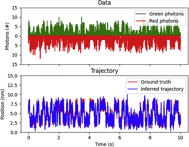
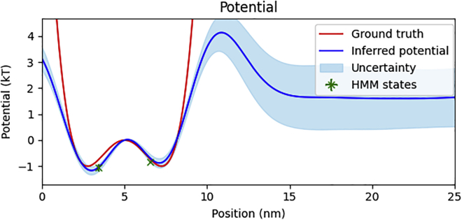
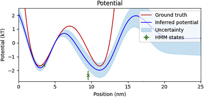
We first analyzed simulated data using a simple double-well potential energy landscape. Values used for the simulation can be found in the supporting material. Fig. 3 shows the data and the trajectory we infer. Fig. 4 shows the SKIPPER-FRET potential energy landscape, the ground-truth potential energy landscape, and the state energies inferred using a Bayesian HMM. The HMM does not infer full potential energy landscapes but rather just the energy and the pair distance of each state (with the added advantage that, both here and elsewhere, we provide the HMM a number of states consistent with the number of potential well minima). As such, we cannot plot a full potential landscape for the HMM results and instead plot point estimates, with uncertainties, indicating the pair distance and energy levels of each state. Indeed, methods that exist to approximate barrier heights between states through such methods necessarily rely on knowledge of other internal parameters of the system such as the friction coefficient and the curvature of the potential at points of inflection (38) (see supporting material) (3.2). We note that in order to compare our method against the ground truth in Fig. 4, we must define a common zero-point energy. Since only potential energy differences (not absolute values) are physical, the reference can be chosen arbitrarily. For our first data set, we chose the point of zero potential energy to be the top of the barrier between the wells.

Figure 3.

Demonstration on simulated data. Here, we demonstrate our method on simulated data. The top shows the raw data from the experiment including red and green photon counts binned every millisecond. The bottom shows the inferred pair distance trajectory (blue) with the ground-truth pair distance trajectory (red). To see this figure in color, go online.

Figure 4.

Simulated potential energy landscape. We show our inferred potential energy landscape (blue) with uncertainty (light blue) against the ground-truth potential energy landscape used in the simulation (red). We additionally plot markers, with uncertainty, indicating the inferred state energy and pair distance using the HMM method (green). The common point of zero potential energy was set at the top of the barrier at 5 nm. To see this figure in color, go online.

As seen in Fig. 3, the SKIPPER-FRET inferred pair distance trajectories are largely consistent with ground-truth trajectory. To be more quantitative, we note in Fig. 4 that our inferred potential energy landscape well minima and barrier height locations fall within 0.2 nm of the ground truth. The inferred well energies were accurate within $0.1kT$ ($-1.2\pm 0.1$ and $-0.9\pm 0.1kT$ versus $-1$ and $-1kT$). We additionally learned a friction coefficient of $0.033\pm 0.002\mathrm{g}/\mathrm{s}$, which is accurate within 12%.

Note that because we can learn the potential only up to a constant, and since we set by hand a point of zero potential energy (the location at which the potential is equal to zero), uncertainty propagation deserves special attention. At the point of zero potential, the potential is precisely defined as zero with no associated uncertainty. As such, the uncertainty in the potential can only grow as we move away from the point of zero potential. In regions with an abundance of data, the uncertainty grows more slowly, while in regions where there are fewer data points, the uncertainty grows more rapidly. Thus, it is the rate of change of the uncertainty that depends on the quantity of data. Put differently, since the potential is the integral of the force, the uncertainty in the potential is the integral of uncertainty in the force. (1.2, 3.6).

We further note from Fig. 4 that while the energies inferred using a Bayesian HMM match the energies learned using SKIPPER-FRET, the pair distances inferred using the HMM deviate from both the ground truth and SKIPPER-FRET well minima. This is on account of the fact that the HMM ascribes a single specified pair distance to what is, in reality, a continuous range of pair distances near potential well minima. To estimate a single specified pair distance, the HMM finds itself effectively averaging the FRET efficiencies over those portions of the trajectory it deems as belonging to one state. This effective pair distance averaging is further complicated when the pair distance trajectory crosses a barrier, in which case the HMM must somehow ascribe the dynamics when surmounting the barrier, which it cannot model, to one of the states.

Next, we analyzed simulated data from a double-well potential where the far rightmost well is centered beyond the range of traditional smFRET measurements (at distance $>2R_0$, where less than 2% of absorbed photons are transferred to the acceptor). Such a potential mimics the data that we expect to see from the binding experiments we later analyze. Fig. 5 shows results where the point of zero potential energy is set at the bottom of the leftmost well. As seen in Fig. 5, our method is able to infer the shape of the left well (where most photons are collected) and still manages to deduce, albeit with reduced accuracy, the shape of the barrier and the far well. The ground-truth potential is enclosed within the uncertainty regions (one standard deviation) of our estimates at almost every point along the left well. Our method further infers a barrier height of about 2.5 kT, which is within 0.5 kT of the ground-truth barrier height (2.9 kT). On the right side of the barrier, where the FRET efficiency drops dramatically and we therefore have less information to inform the shape of the potential inferred, our estimate deviates from the ground truth with a correspondingly growing uncertainty.

Figure 5.

Simulated potential energy landscape when one barrier is far from the characteristic FRET distance. Here, we analyze data simulated using an energy landscape in which one of the wells is outside of the characteristic FRET range. We compare our inferred potential energy landscape with the potential energy landscape inferred using the Bayesian HMM as well as the ground truth. We show our inferred potential energy landscape (blue) with uncertainty (light blue) against the ground-truth potential energy landscape used in the simulation (red). We additionally plot markers, with uncertainty, indicating the inferred state energy and pair distance using the HMM method (green). The common point of zero potential energy was set at the bottom of the leftmost well at 2.87 nm. To see this figure in color, go online.

Roughly speaking, we do not expect to be able to accurately infer the potential at locations where the number of expected photons is of order unity. We can approximate the maximum distance we can probe, $x_{\text{MAX}}$, as the largest distance where the number of photons transferred from the donor to the acceptor (given by the excitation rate, ${\lambda }_X$ multiplied by the probability of FRET is greater than or approximately equal to unity). In other words, $1\approx {\lambda }_X{(1+(x_{\text{MAX}}/R_0)}^6)-1$, and thus

$$x_{\text{MAX}}\approx R_0{\left({\lambda }_X-1\right)}^{1/6}\text{.}$$ (21)

Our method additionally infers a friction coefficient of $0.035\pm 0.02\mathrm{g}/\mathrm{s}$, which is accurate within 20% of the ground truth. When comparing this with the HMM method, we again see that the HMM method and SKIPPER-FRET estimate similar energies but different well locations.

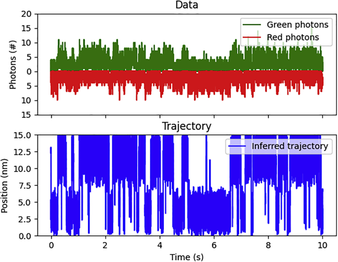
After successfully testing SKIPPER-FRET on simulated data, we now move on to the analysis of experimental data. In Fig. 6, we show the inferred trajectory by applying our method to data from ACTR-NCBD binding-unbinding experiments (37). Based on independent analysis (38,40,41), we expect to find two states corresponding to bound and unbound states. Furthermore, looking at the raw data in the top panel of Fig. 6, we immediately notice that there are alternating sections of high and low FRET efficiency in what appears to be two states. The corresponding inferred pair distance trajectory, as seen in the bottom panel of Fig. 6, also alternates between two levels as expected.

Figure 6.

Demonstration on NCBD-ACTR. Here, we demonstrate our method on data probing the energy landscape of NCBD-ACTR binding. (Top) shows the raw data from the experiment including red and green photon counts. (Bottom) shows the inferred pair distance trajectory (blue). To see this figure in color, go online.

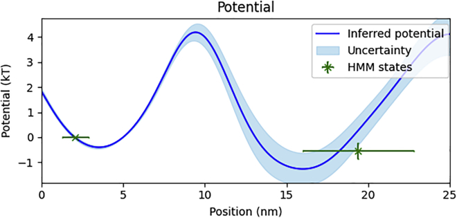
We also show the inferred potential energy landscape in Fig. 7. Indeed, as expected, we recover a double well. The left well in Fig. 7 can be interpreted as the binding energy between ACTR and the NCBD, while the right well can be interpreted as the chemical potential energy required to remove NCBD from a volume surrounding the ACTR.

Figure 7.

NCBD-ACTR potential energy landscape. Here, we compare our inferred potential energy landscape with the relative potential energy landscape inferred using standard HMM methods. We show our inferred potential energy landscape (blue) with uncertainty (light blue). We additionally plot markers, with uncertainty, indicating the inferred state energy and pair distance using the HMM method (green). To see this figure in color, go online.

As the true energy landscape for ACTR-NCBD binding is unknown, we compare our results with the energy landscape inferred using a two state Bayesian HMM model with the same likelihood model as SKIPPER-FRET (see supporting material section S0.10). As seen in Fig. 7, the energies inferred using the HMM method fall within our uncertainty regions, but the position of the wells inferred using SKIPPER-FRET differ from those inferred using the HMM method. As explained earlier, this arises because, fundamentally, the HMM attempts to reconcile its discrete-state picture with the Langevin model’s continuous formulation. As the HMM method does not provide barrier height, we cannot naturally compare the barrier inferred using SKIPPER-FRET within the HMM paradigm without additional information (see supporting material). Lastly, we infer a friction coefficient of $1.54\pm 0.05\text{mg}/\mathrm{s}$. While we lack ground truth to verify our estimate, we can say that this value is consistent with dimensional analysis estimates from the data (see supporting material).

Discussion

Inferring accurate potential energy landscapes is a critical step toward unraveling key biophysical phenomena including protein folding (11), binding (3,8), and the dynamics of molecular motors (16). Here, we have developed a method orthogonal to the HMM paradigm to include continuous states that also yields barrier heights. We benchmarked our method on simulated and experimental data.

We showed that, if warranted, we can avoid making the discrete-state assumption inherent to HMMs, while the HMM only has access to energy barriers between states if we supply it with preexisting knowledge of the internal parameters of the reaction coordinate or if there are at least two data sets taken at different temperatures (see supporting material). This is despite any single data set already encoding this information.

Key to our inference algorithm is the SKI-GP, which allows us to sample the potential energy landscape from a prior over all continuous curves while avoiding the costly cubic scaling requirements of a standard GP. Specifically, with the SKI-GP prior, we are able to define inducing point locations, ${\mathit{x}}_{1:M}^{\ast }$, separate from the trajectory, ${\mathbf{x}}_{1:N}$, to avoid calculating a new covariance matrix, $\mathit{K}$, and its inverse, ${\mathit{K}}^{-1}$, at each iteration of our Gibbs sampler, thereby saving considerable computational time. This would not be possible using standard GP techniques.

Moving forward, there are ways in which we may improve SKIPPER-FRET. Firstly, our method, as it stands, deals with smFRET data from continuously illuminated sources. However, many smFRET experiments work using pulsed excitation (23,42). We could modify our measurement model (Eq. 6 to Eq. 7) to accommodate pulsed illumination by swapping the Poisson distribution, which assumes exponential waiting times between excitation, for a Binomial distribution, compatible with fixed window excitations.

Also, our method deals with dynamics along a single reaction coordinate assumed to be equivalent to the FRET pair distance. However, one can imagine situations in which the system’s dynamics are probed along an axis partly orthogonal to the FRET pair distance (43,44) in a multidimensional incarnation of FRET with, say, one donor and multiple acceptor labels. For example, even in the case of ACTR binding to the NCBD, as analyzed in this manuscript, the ACTR may rotate with respect to the NCBD during binding. Cases with multiple degrees of freedom are traditionally studied using multicolor smFRET (44,45,46,47) or by pairing data analysis with molecular dynamics simulations (44,48). In principle, one could use SKIPPER-FRET to infer potentials along degrees of freedom orthogonal to the FRET distance by including some mapping from the desired degree of freedom to the FRET pair distance in equation (8). As the FRET pair distance is often not directly tied to the reaction coordinate (42,49), this may be a promising direction for future work.

Along these same lines, while our focus has, so far, been on learning one-dimensional potentials and demonstrating that we can learn barriers and potential shapes, avoiding the costly cubic scaling of standard GPs is also critical in deducing higher-dimensional potentials. For instance, an HMM may, for example, distinguish between a fully connected and linear three-state model. Here, our one-dimensional reduction would need to be augmented to two dimensions in order for us to deduce these types of higher-dimensional features. Deducing features, such as potential ridges and valleys, in higher dimensions is the object of future work.

Author contributions

J.S.B. wrote the manuscript and carried out all derivations, coding, and inference. S.P. conceived the project and oversaw all aspects of the project.

Editor: Diane Lidke.

Data and code availability

Our analysis code can be found at https://github.com/LabPresse/PotentialsFromFRET.

References

- 1.Phillips R., Kondev J., et al. Garcia H. Garland Science; 2012. Physical Biology of the Cell. [Google Scholar]
- 2.Schuler B., Lipman E.A., Eaton W.A. Probing the free-energy surface for protein folding with single-molecule fluorescence spectroscopy. Nature. 2002;419:743–747. doi: 10.1038/nature01060. [DOI] [PubMed] [Google Scholar]
- 3.Yan Z., Wang J. Funneled energy landscape unifies principles of protein binding and evolution. Proc. Natl. Acad. Sci. USA. 2020;117:27218–27223. doi: 10.1073/pnas.2013822117. [DOI] [PMC free article] [PubMed] [Google Scholar]
- 4.Weistuch C., Pressé S. Spatiotemporal organization of catalysts driven by enhanced diffusion. J. Phys. Chem. B. 2018;122:5286–5290. doi: 10.1021/acs.jpcb.7b06868. [DOI] [PubMed] [Google Scholar]
- 5.Makarov D.E. Barrier crossing dynamics from single-molecule measurements. J. Phys. Chem. B. 2021;125:2467–2476. doi: 10.1021/acs.jpcb.0c10978. [DOI] [PubMed] [Google Scholar]
- 6.Tiwary P., Parrinello M. From metadynamics to dynamics. Phys. Rev. Lett. 2013;111:230602. doi: 10.1103/PhysRevLett.111.230602. [DOI] [PubMed] [Google Scholar]
- 7.Wang J., Ferguson A.L. Nonlinear reconstruction of single-molecule free-energy surfaces from univariate time series. Phys. Rev. E. 2016;93:032412. doi: 10.1103/PhysRevE.93.032412. [DOI] [PubMed] [Google Scholar]
- 8.Wang J., Verkhivker G.M. Energy landscape theory, funnels, specificity, and optimal criterion of biomolecular binding. Phys. Rev. Lett. 2003;90:188101. doi: 10.1103/PhysRevLett.90.188101. [DOI] [PubMed] [Google Scholar]
- 9.Chu X., Gan L., Wang E., Wang J. Quantifying the topography of the intrinsic energy landscape of flexible biomolecular recognition. Proc. Natl. Acad. Sci. USA. 2013;110:E2342–E2351. doi: 10.1073/pnas.1220699110. [DOI] [PMC free article] [PubMed] [Google Scholar]
- 10.Schuler B., Eaton W.A. Protein folding studied by single-molecule fret. Curr. Opin. Struct. Biol. 2008;18:16–26. doi: 10.1016/j.sbi.2007.12.003. [DOI] [PMC free article] [PubMed] [Google Scholar]
- 11.Dill K.A., MacCallum J.L. The protein-folding problem, 50 years on. Science. 2012;338:1042–1046. doi: 10.1126/science.1219021. [DOI] [PubMed] [Google Scholar]
- 12.Hänggi P., Talkner P., Borkovec M. Reaction-rate theory: fifty years after kramers. Rev. Mod. Phys. 1990;62:251–341. [Google Scholar]
- 13.Berezhkovskii A.M., Dagdug L., Bezrukov S.M. Mean direct-transit and looping times as functions of the potential shape. J. Phys. Chem. B. 2017;121:5455–5460. doi: 10.1021/acs.jpcb.7b04037. [DOI] [PMC free article] [PubMed] [Google Scholar]
- 14.Bessarab P.F., Uzdin V.M., Jónsson H. Potential energy surfaces and rates of spin transitions. Z. Phys. Chem. 2013;227:1543–1557. [Google Scholar]
- 15.Wang H., Oster G. Energy transduction in the f 1 motor of atp synthase. Nature. 1998;396:279–282. doi: 10.1038/24409. [DOI] [PubMed] [Google Scholar]
- 16.Toyabe S., Ueno H., Muneyuki E. Recovery of state-specific potential of molecular motor from single-molecule trajectory. EPL. 2012;97:40004. [Google Scholar]
- 17.Clegg R.M. Fluorescence resonance energy transfer. Curr. Opin. Biotechnol. 1995;6:103–110. doi: 10.1016/0958-1669(95)80016-6. [DOI] [PubMed] [Google Scholar]
- 18.Clegg R.M. Reviews in Fluorescence 2006. Springer; 2006. The history of fret; pp. 1–45. [Google Scholar]
- 19.Lerner E., Cordes T., et al. Weiss S. Toward dynamic structural biology: two decades of single-molecule förster resonance energy transfer. Science. 2018;359 doi: 10.1126/science.aan1133. eaan1133. [DOI] [PMC free article] [PubMed] [Google Scholar]
- 20.Ziv G., Haran G. Protein folding, protein collapse, and tanford’s transfer model: lessons from single-molecule fret. J. Am. Chem. Soc. 2009;131:2942–2947. doi: 10.1021/ja808305u. [DOI] [PMC free article] [PubMed] [Google Scholar]
- 21.Mazal H., Haran G. Single-molecule fret methods to study the dynamics of proteins at work. Curr. Opin. Biomed. Eng. 2019;12:8–17. doi: 10.1016/j.cobme.2019.08.007. [DOI] [PMC free article] [PubMed] [Google Scholar]
- 22.Lindsay S. OUP Oxford; 2009. Introduction to Nanoscience. [Google Scholar]
- 23.Hellenkamp B., Schmid S., et al. Hugel T. Precision and accuracy of single-molecule fret measurements-a multi-laboratory benchmark study. Nat. Methods. 2018;15:669–676. doi: 10.1038/s41592-018-0085-0. [DOI] [PMC free article] [PubMed] [Google Scholar]
- 24.Bishop C.M. Springer; 2006. Pattern Recognition and Machine Learning. [Google Scholar]
- 25.Pressé S., Lee J., Dill K.A. Extracting conformational memory from single-molecule kinetic data. J. Phys. Chem. B. 2013;117:495–502. doi: 10.1021/jp309420u. [DOI] [PMC free article] [PubMed] [Google Scholar]
- 26.Pressé S., Peterson J., et al. Dill K. Single molecule conformational memory extraction: P5ab rna hairpin. J. Phys. Chem. B. 2014;118:6597–6603. doi: 10.1021/jp500611f. [DOI] [PMC free article] [PubMed] [Google Scholar]
- 27.Sgouralis I., Madaan S., et al. Pressé S. A bayesian nonparametric approach to single molecule forster resonance energy transfer. J. Phys. Chem. B. 2019;123:675–688. doi: 10.1021/acs.jpcb.8b09752. [DOI] [PMC free article] [PubMed] [Google Scholar]
- 28.McKinney S.A., Joo C., Ha T. Analysis of single-molecule fret trajectories using hidden markov modeling. Biophys. J. 2006;91:1941–1951. doi: 10.1529/biophysj.106.082487. [DOI] [PMC free article] [PubMed] [Google Scholar]
- 29.Reif F. Waveland Press; 2009. Fundamentals of Statistical and Thermal Physics. [Google Scholar]
- 30.Sgouralis I., Pressé S. Icon: an adaptation of infinite hmms for time traces with drift. Biophys. J. 2017;112:2117–2126. doi: 10.1016/j.bpj.2017.04.009. [DOI] [PMC free article] [PubMed] [Google Scholar]
- 31.Zhang Y., Jiao J., Rebane A.A. Hidden markov modeling with detailed balance and its application to single protein folding. Biophys. J. 2016;111:2110–2124. doi: 10.1016/j.bpj.2016.09.045. [DOI] [PMC free article] [PubMed] [Google Scholar]
- 32.Wilson A., Nickisch H. International Conference on Machine Learning. PMLR; 2015. Kernel interpolation for scalable structured Gaussian processes (kiss-gp) pp. 1775–1784. [Google Scholar]
- 33.Zwanzig R. Oxford university press; 2001. Nonequilibrium Statistical Mechanics. [Google Scholar]
- 34.Bryan J.S., 4th, Basak P., et al. Pressé S. Inferring potential landscapes from noisy trajectories of particles within an optical feedback trap. iScience. 2022;25:104731. doi: 10.1016/j.isci.2022.104731. [DOI] [PMC free article] [PubMed] [Google Scholar]
- 35.Bryan J.S., 4th, Sgouralis I., Pressé S. Inferring effective forces for Langevin dynamics using Gaussian processes. J. Chem. Phys. 2020;152:124106. doi: 10.1063/1.5144523. [DOI] [PMC free article] [PubMed] [Google Scholar]
- 36.Williams C.K., Rasmussen C.E. Vol. 2. MIT press Cambridge; 2006. (Gaussian Processes for Machine Learning). [Google Scholar]
- 37.Zosel F., Soranno A., et al. Schuler B. Depletion interactions modulate the binding between disordered proteins in crowded environments. Proc. Natl. Acad. Sci. USA. 2020;117:13480–13489. doi: 10.1073/pnas.1921617117. [DOI] [PMC free article] [PubMed] [Google Scholar]
- 38.Sturzenegger F., Zosel F., et al. Schuler B. Transition path times of coupled folding and binding reveal the formation of an encounter complex. Nat. Commun. 2018;9:4708. doi: 10.1038/s41467-018-07043-x. [DOI] [PMC free article] [PubMed] [Google Scholar]
- 39.Zosel F., Mercadante D., Schuler B., et al. A proline switch explains kinetic heterogeneity in a coupled folding and binding reaction. Nat. Commun. 2018;9:3332. doi: 10.1038/s41467-018-05725-0. [DOI] [PMC free article] [PubMed] [Google Scholar]
- 40.Saurabh A., Safar M., et al. Pressé S. Single photon smfret. i. theory and conceptual basis. bioRxiv. 2022 doi: 10.1101/2022.07.20.500887. Preprint at. [DOI] [PMC free article] [PubMed] [Google Scholar]
- 41.Saurabh A., Safar M., et al. Pressé S. Single photon smfret. ii. application to continuous illumination. bioRxiv. 2022 doi: 10.1101/2022.07.20.500888. Preprint at. [DOI] [PMC free article] [PubMed] [Google Scholar]
- 42.Baltierra-Jasso L.E., Morten M.J., Magennis S.W. Sub-ensemble monitoring of dna strand displacement using multiparameter single-molecule fret. ChemPhysChem. 2018;19:551–555. doi: 10.1002/cphc.201800012. [DOI] [PubMed] [Google Scholar]
- 43.Harris N., Botello E., et al. Kiang C.-H. Is end-to-end distance a good reaction coordinate? Biophys. J. 2009;96:290a. [Google Scholar]
- 44.Kolimi N., Pabbathi A., et al. Alper J. Out-of-equilibrium biophysical chemistry: the case for multidimensional, integrated single-molecule approaches. J. Phys. Chem. B. 2021;125:10404–10418. doi: 10.1021/acs.jpcb.1c02424. [DOI] [PMC free article] [PubMed] [Google Scholar]
- 45.Feng X.A., Poyton M.F., Ha T. Multicolor single-molecule fret for dna and rna processes. Curr. Opin. Struct. Biol. 2021;70:26–33. doi: 10.1016/j.sbi.2021.03.005. [DOI] [PMC free article] [PubMed] [Google Scholar]
- 46.Wang L., Tan W. Multicolor fret silica nanoparticles by single wavelength excitation. Nano Lett. 2006;6:84–88. doi: 10.1021/nl052105b. [DOI] [PMC free article] [PubMed] [Google Scholar]
- 47.Yoo J., Kim J.-Y., et al. Chung H.S. Fast three-color single-molecule fret using statistical inference. Nat. Commun. 2020;11:3336. doi: 10.1038/s41467-020-17149-w. [DOI] [PMC free article] [PubMed] [Google Scholar]
- 48.Torella J.P., Holden S.J., et al. Kapanidis A.N. Identifying molecular dynamics in single-molecule fret experiments with burst variance analysis. Biophys. J. 2011;100:1568–1577. doi: 10.1016/j.bpj.2011.01.066. [DOI] [PMC free article] [PubMed] [Google Scholar]
- 49.Hu T., Morten M.J., Magennis S.W. Conformational and migrational dynamics of slipped-strand dna three-way junctions containing trinucleotide repeats. Nat. Commun. 2021;12:204. doi: 10.1038/s41467-020-20426-3. [DOI] [PMC free article] [PubMed] [Google Scholar]
Associated Data
This section collects any data citations, data availability statements, or supplementary materials included in this article.
Supplementary Materials
Data Availability Statement