Kalman-based compartmental estimation for covid-19 pandemic using advanced epidemic model

Abstract

The practicality of administrative measures for covid-19 prevention is crucially based on quantitative information on impacts of various covid-19 transmission influencing elements, including social distancing, contact tracing, medical facilities, vaccine inoculation, etc. A scientific approach of obtaining such quantitative information is based on epidemic models of $SIR$ family. The fundamental $SIR$ model consists of S-susceptible, I-infected, and R-recovered from infected compartmental populations. To obtain the desired quantitative information, these compartmental populations are estimated for varying metaphoric parametric values of various transmission influencing elements, as mentioned above. This paper introduces a new model, named $SEIRRPV$ model, which, in addition to the S and I populations, consists of the E-exposed, $R_e$-recovered from exposed, R-recovered from infected, P-passed away, and V-vaccinated populations. Availing of this additional information, the proposed $SEIRRPV$ model helps in further strengthening the practicality of the administrative measures. The proposed $SEIRRPV$ model is nonlinear and stochastic, requiring a nonlinear estimator to obtain the compartmental populations. This paper uses cubature Kalman filter (CKF) for the nonlinear estimation, which is known for providing an appreciably good accuracy at a fairly small computational demand. The proposed $SEIRRPV$ model, for the first time, stochastically considers the exposed, infected, and vaccinated populations in a single model. The paper also analyzes the non-negativity, epidemic equilibrium, uniqueness, boundary condition, reproduction rate, sensitivity, and local and global stability in disease-free and endemic conditions for the proposed $SEIRRPV$ model. Finally, the performance of the proposed $SEIRRPV$ model is validated for real-data of covid-19 outbreak.

Graphical abstract

1. Introduction

Covid-19 is an airborne transmitted viral infection caused by severe acute respiratory syndrome coronavirus-2, often abbreviated as SARS-CoV-2 [1]. It originated from Wuhan, the capital city of the Hubei province of the People’s Republic of China [2]. The World Health Organization (WHO) officially declared the covid-19 an international public health emergency on January 30, 2020. Since the day of its inception, coronavirus has infected close to half a billion people and killed close to 6 million people worldwide (till February 2022) [3], [4]. It also forced almost every country across the globe to impose a strict lockdown to reduce infection rates. On the contrary, the lockdown further caused substantial economic losses to the entire world [5]. Furthermore, recent research suggests that coronavirus mutates its genome sequence resulting in new variants that make the vaccine less effective over time [6], [7].

In this challenging period, researchers developed knowledge-based mathematical analysis for analyzing the disease dynamics as in [8], [9], and [10] to reduce the burden on medical infrastructure. It is also possible that aggressive non-pharmaceutical interventions (nPIs) may cause the country’s financial burden to increase [5]. Therefore, we should focus on nPIs with a minimal financial burden. An effective solution in preventing the covid-19 spread may be an efficient vaccine. However, in the absence of efficient vaccines, the administrative authorities may consider dynamical model-based analytical results in order to frame appropriate administrative strategies and guidelines for public.

The works of [11], [12], and [13] appear in the literature to characterize the repercussions of diseases from mathematical models. Among such mathematical models, compartmental-based models are popular [14]. They categorize total population into different compartments based on the infection level in an individual. The simplest form of compartmental-based model is susceptible–infected–recover ($SIR$) model [15]. During modeling, $SIR$ model considers a few parameters, such as infection rate, recovery rate, and recovery rate from disease.

It is expected that model ($SIR$ model) analysis-based strategy making should be superior if the models comprise of more parameters. With this motivation, the later developments incorporated more compartments, including susceptible (S), exposed (E), infected (I), recovered from exposed (R), recovered from infected (R), passed away (P), and vaccinated individual (V) compartments. With different combinations of such compartments, various models, including $SIRP$ [16], [17], $SEIR$ [18], $SEIRP$ [19], $SEIRRP$ [20], $SIRV$ [21] models, are introduced in the recent literature. These models are nonlinear in order to characterize the nonlinear disease dynamics. Moreover, these models become stochastic in order to characterize the modeling errors and uncertainties of the disease dynamics. Apart from these contributions, [22] introduced a data fitting-based model for analyzing the effect of additional controls in the strategy making for covid prevention. Furthermore, [23], and [24] introduced some advancements in the estimation algorithm for accurately estimating the compartmental populations.

As discussed above, various contributions appear for the model-based analysis of covid-19 spread. However, they lack in different aspects, requiring serious advancements. For example, [16], [17], [19], [22], [23], and [24], assume that the recovery of individuals is consistent for the exposed (asymptomatic infected) and infected populations. In contrast, different covid variants have shown different trends of their recoveries. Adding to this difficulty further, the explicit information on recovery of exposed individual is infeasible, particularly for a large population, as it requires very broad public screening [20], [25]. Thus, in order to monitor the exposed population, Giordano et al. [25] introduced a deterministic epidemic model. This contribution, however, fails to address the model and disease uncertainties due to its deterministic nature. Furthermore, none of the previously discussed contributions consider the exposed and vaccinated populations in a single model, resulting in poor accuracy, particularly after considering the developments of various vaccines, including Pfizer, Covaxin, and AstraZeneca.

Literature on epidemic model state estimation witnesses recursive least square estimation [20], maximum likelihood method [23], [26], [27], and Markov chain Monte-Carlo [13]. Sameni et al. [20] used recursive least square estimation method by minimizing linear least square cost function. These methods are often dependent on accuracy of the measurement data. Hasan et al. [16] developed an extended Kalman filter (EKF)-based $SIRP$ model. In EKF, the partial derivatives are computed to locally linearize the highly nonlinear epidemic model, which does not guarantee the optimality and stability of the estimation for highly nonlinear system. Later unscented Kalman filter (UKF) integrated epidemic model replaces Jacobian matrix-based linearization with simpler and more stable unscented transformation based numerical approximations to linearize nonlinear disease dynamics model [17]. A $SEIRP$ model was proposed to investigate the dynamic behavior of the COVID-19 pandemic [19]. Later, Xinhe et al. developed an EKF-based estimation method for $SEIRP$ epidemic model by incorporating reinfection rate to estimate the covid-19 compartments [24]. Similarly, Jialu et al. introduced an EKF-based estimation of $SEIRP$ model, where the parameters of the model were using the maximum likelihood method [23]. The above discussed estimation methods, such as the EKF, UKF, and their extensions, used in the [16], [17], [23], [24], are known for their poor accuracy and stability. Thus, introducing an efficient estimation method can further improve the accuracy.

Summarizing the above discussions, we highlight the motivations of the manuscript below:

• •Consider the exposed and infected populations separately in order to address their inconsistent recovery pattern.
• •Consider the stochastic nature of the model in order to address the limitations of [25] in the manuscript.
• •Consider the exposed and vaccinated populations in a single model, which is yet not considered in the literature.
• •Use an advanced estimation technique, like the CKF, for estimating the compartmental populations with improved accuracy.
• •Finally, the motivation of the paper is to improve the accuracy of the model-based covid-19 spread analysis by accomplishing the above mentioned motivations.

In order to accomplish the above mentioned motivations, we use an advanced $SIR$ model and a popularly known estimation technique named cubature Kalman filter (CKF) to derive analytical conclusions helpful in non-pharmaceutical policy-making. We include various coronavirus disease impacting parameters, such as infection rate, recovery rate, reinfection rate, mortality rate, incubation rate, recovery rate of exposed group, and vaccination rate to model complex covid-19 disease dynamics. The model considers seven stages of infections: susceptible (S), exposed (E), infected (I), recovered from exposed ($R_e$), recovered from infected (R), passed away (P), and vaccinated (V) population; abbreviated as $SEIRRPV$ epidemic model. Henceforth, we will refer to the advanced $SIR$ model as $SEIRRPV$ model in the acronym form of its compartment. To validate, a mathematical analysis of the proposed epidemic model is demonstrated, which identifies the non-negativity, uniqueness, boundary condition, basic reproduction rate, sensitivity analysis, and stability analysis. A stochastic $SEIRRPV$ model is then combined with a novel estimation technique, the cubature Kalman filter (CKF), to derive analytical conclusions about the epidemic transmission. The CKF is a nonlinear Bayesian approximation filtering method, which is performed in prediction and update steps. The implementation of the prediction and update steps involves intractable integrals. The CKF uses third-degree spherical cubature rule for approximating the intractable integrals. Finally, we compared our results with existing $SIR$, $SIRP$, $SEIRP$, $SEIRRP$, $SIRV$ models [20], [21], and [28]. The meaning of these models can be derived from the descriptions of every word provided. Please note that ‘recover’ represents those recovered from covid-19 infection for $SIR$, $SIRP$, $SEIRP$, and $SIRV$ models where exposed compartment is not considered.

Rest of the paper is organized as follows: A brief discussion on the proposed compartmental-based $SEIRRPV$ epidemic model is provided in Section 2. Problem formulation is described in Section 3. Mathematical analysis for the epidemic model is presented in Section 4. Cubature Kalman filtering method is derived in Section 5 and simulation of the pandemic outbreak for two cases in Section 6. Finally, we present the discussion in Section 7 and concluding remarks in Section 8.

2. Compartmental based $\mathbf{SEIRRPV}$ model for analyzing covid-19 spread

This section gives an overview of the compartmental-based epidemic model used to analyze the spread of covid-19. In general, the behavior of real-life systems or processes is complex, and modeling their exact dynamics is challenging. However, in many cases, the physical laws are well established in the literature to derive an approximated model, e.g., the laws of motion can be used for approximate modeling of the motion of a moving object [15]. On the other hand, modeling dynamics of a biological process, such as the transmission of a new pandemic, is complex and lacks well-established physical laws characterizing their dynamics. The covid-19 transmissibility is dynamic and ever-changing. It is new and unique for the scientific community, and no physical law is yet developed to define its transmission rate and other behavior precisely. In such cases, the standard mathematical models are established in the literature for modeling disease behavior based on certain hypotheses applied to the pandemic behavior. Before introducing the proposed $SEIRRPV$ model, we mention the following hypotheses on any pandemic [14], [29]:

• (i)The disease is contagious and spreads through direct and indirect contact or even airborne transmission.
• (ii)The population remains constant during the period of the study. The deaths (excluding those caused by pandemic) and births during the study duration are ignored. It is worth mentioning that these numbers are expected to be small compared to the total population.
• (iii)There may be some latency period during which an infected individual is not infectious. Similarly, There may be an exposure period during which an individual may be both infected and contagious but does not show any visible symptoms, $i.e.$, asymptomatic.
• (iv)Every individual in the considered population has the same immunity.
• (v)Every individual in the considered population interacts equally with others in other compartments.

It should be mentioned that the hypotheses may not be unique across the practitioners. However, the resulting accuracy and the model complexity should be key factors in specifying a particular set of hypotheses.

The above mentioned hypotheses are generally common for all compartmental-based modeling. A deterministic $SEIRRPV$ model follows these hypotheses. Any modeling study comes with inherent limitations. Here, hypotheses (ii), (iv), and (v) condition are not true for coronavirus epidemic. However, we can approximate a study of shorter duration and associated uncertainty in our model. We consider the scenario of covid-19 pandemic in Delhi, the capital city of India, with a population of 32 million. We implemented the proposed model to estimate the disease transmission in Delhi between 17 January 2021 and 26 April 2021. The simulation study period is important because Delhi witnessed its second wave from March and stretched to June 2021. There was a covid outbreak throughout the city of Delhi. Hence, our assumption stands true that the entire population is equally susceptible to the covid-19 pandemic. Although the birth rate (approximately 0.003% of total population) and natural death rate (0.03% of total population) are negligible compared to the total population of Delhi (approximately 32 million), the imperfection in these models could result in uncertainty in the predictive capability of covid-19. Therefore, authors remodeled the deterministic epidemic model as a stochastic-based $SEIRRPV$ epidemic model. In stochastic systems, there is no disease-endemic state, so persistence of the disease cannot be observed.

2.1. Parameters involved in covid-19 pandemic

The real-world scenarios, such as medical infrastructure, geographic demographics, social structure, public awareness, government strategies, etc., may be linked to a mathematical model. These epidemic models estimate different compartments and simulate various parameters influencing the transmission of the covid-19 pandemic. Some of these parameters have been explained below.

2.1.1. Infection rate ($\alpha$)

As mentioned in the previous section, the $\alpha$ number of susceptible people get infected with covid-19 from an infected or exposed individual per unit of time. The covid-19 disease can transmit through direct and indirect contact and airborne transmission. So infection rate parameter considers the level of social interaction, population density, environment healthiness, and social cleanliness. A high contact rate increases the infected population at a faster pace. However, strict measures and social awareness can slow down the transmission of the SARS-COV-2 virus even in densely populated cities or places having poor healthcare facilities. One such example is Asia’s largest slum bearer, Dharavi, which successfully controlled the pandemic by stricter social measures imposed by Brihanmumbai Municipal Corporation (BMC), Maharastra, India [30], as acknowledged by the world health organization (WHO). Government authority’s decisions include critical social distancing at the workplace, masks in populated areas, protection against virulence and lockdown, and others.

2.1.2. Recovery rate ($\beta$)

It is the rate at which infected individuals are reported to have recovered on a given day. The speedy recovery of people depends on the healthcare facilities and medication they get. Hence state hospitalization facilities, number of intensive care units (ICUs), availability of clinical drugs, transportation facilities, etc., impact the recovery speed for the pandemic. The value of $\beta$ may be different for all pandemics. One influenza-infected individual gets ill for 3–7 days (mean time =5 days), so the recovery rate $\beta$ is 1/5 [20].

2.1.3. Reinfection rate ($\gamma$)

It is the rate at which recovered individuals get reinfected with covid-19. In recent times, few covid-19 fully vaccinated people have also been infected. So, vaccination does not make an individual fully immunized. Thus $\gamma$ is the inverse of the immunity rate. It is otherwise called as immunity loss rate. Preliminary studies claim the immunity rate for covid-19 stands for up to 4 months [31]. In $SEIRP$, $SEIRRP$, and $SEIRRPV$-models, we have segregated infected people into exposed and infected compartments. Recovered people may get exposed or infected with covid-19. In $SEIRP$, $SEIRRP$, and $SEIRRPV$-models, reinfection rate terms are specified as ${\gamma }_e$, and $\gamma$, respectively. Moreover, we have one compartment to address contaminated people (‘infected’ compartment), so the reinfection rate for $SIR$, $SIRV$, and $SIRP$-models, is $\gamma$.

2.1.4. Mortality rate ($\mu$)

The covid-19 pandemic has caused more than 5.8 million human deaths (updated on February 2022) [3]. The mortality rate of the pandemic is the ratio of the daily number of deceased people to the total infected population on the same day. Hence the influencing constraints for mortality rate are the same as infection rate.

2.1.5. Incubation rate ($\kappa$)

The transition of an asymptomatically infected individual (E) to be symptomatically infectious individual (I) is called an incubation rate. In some cases, people are infected and contagious. Still, they do not show any symptoms, or they are medically declared as covid-19 -ve due to the poor medical facility or by an error in real-time polymerase chain reaction (RTPCR) test or antigen test [32]. These exposed people act as an active virus carriers, and the host may die or recover in both cases. So screening policies, contact tracing, etc., like aspects may influence $\kappa$.

2.1.6. Recovery rate of exposed group ($\rho$)

It is the rate at which exposed group individuals recover without being infectious. However, it cannot be inspected and needs lab-based proof. It may be considered equal to or greater than $\beta$.

2.1.7. Vaccination rate ($\Omega$)

It is the rate at which people are vaccinated to be immune from the variants of coronavirus. Vaccination drive speed not only provides a weapon to reduce infection rate but also reduces human fatalities. However, vaccine inefficiency, $\nu$, may reduce the vaccine’s effectiveness. During the vaccine testing and clinical trials, its efficiency is evaluated.

2.2. Mathematical representation

We introduce the compartmental models to analyze the covid-19 transmission behavior based on the above mentioned hypotheses. Our model is inspired by the $SIR$ epidemic model with inclusion of other pandemic spread impacting parameters, such as rate of asypmtomatically infection ${\alpha }_e$, infection rate $\alpha$, recovery rate $\beta$, reinfection rate for covid-19 recovered individual from exposed ${\gamma }_e$ and infected compartment $\gamma$, mortality rate $\mu$, incubation rate $\kappa$, recovery rate of exposed population $\rho$. Additionally, the recent vaccine rollout by Pfizer, AstraZeneca, and others will favor the physical epidemic model. Here, vaccination rate, $\Omega$, and vaccination inefficacy, $\nu$, play a vital role in controlling the pandemic. Hence our proposed model is also more diversified in the model formulation of complex disease transmission.

We follow transmission patterns of the pathogens in classified compartments in terms of ordinary differential equations to formulate the proposed $SEIRRPV$ epidemic model. According to the World Health Organization, there are two varieties of people infected by coronavirus: one does not have symptoms (E), and the other does (I). We consider the scenario of covid-19 pandemic in Delhi, the capital city of India, with a population of 32 million. We implemented the proposed model to estimate the disease transmission in Delhi between 17 January 2021 and 26 April 2021. The period of the simulation study is important in the fact that Delhi witnessed its second wave of covid-19 pandemic from March and stretched up to June of 2021. Here is assumption stands true with the covid-19 pandemic transmission in Delhi, i.e., total population of Delhi is equally susceptible to the covid-19 pandemic.

• (i)Susceptible compartment individual transfer to exposed (E) asymptomatically, and symptomatically, respectively with infection rates of ${\alpha }_e$ and $\alpha$. Additionally, recovered individuals from $R_e$ and $R$ compartments become susceptible with recovery rates ${\gamma }_e$ and $\gamma$, respectively. Further, A small portion of vaccinated population becomes susceptible due to vaccination at a rate of $\Omega$.
• (ii)Population from susceptible (S) and vaccinated (V) compartment transfer to exposed (E) compartment with ${\alpha }_{e}E+\alpha I$ and $\nu {\alpha }_{e}V$, respectively.
• (iii)Incubation rate $\kappa$ of exposed population and $\nu \alpha I$ of vaccinated population coming to the infected (I) compartment from exposed (E) and vaccinated (V) population compartment.
• (iv)Recovered populations from asymptomatically infected or not hospitalized or those populations recovered from covid-19 but got unnoticed by the government data are included in the $R_e$ compartment. It includes the net population of inclusion of recovery rate $\rho$ of exposed population and exclusion of reinfected population at a rate of ${\gamma }_e$.
• (v)$R$ compartment includes individuals $\beta$ rate of infected population (I) by excluding reinfected rate of recovered population (R).
• (vi)Passed away (P) compartment are the mortality rate $\mu$ of infected population (I).
• (vii)Vaccinated population is the net population of vaccinated people from susceptible compartment $S$ with $\Omega$ rate by excluding infected people both symptomatically with $\nu {\alpha }_{e}I$ and asymptomatically infected with $\nu \alpha E$.

We follow the fundamental steps (i)–(vii) to formulate our proposed deterministic epidemic model. The following set of differential equations mathematically represents compartments of the $SEIRRPV$ model.

$$\frac{dS}{dt}=-{\alpha }_{e}SE-\alpha SI+{\gamma }_e{R}_e+\gamma R-\Omega S$$$$\frac{dE}{dt}={\alpha }_{e}SE+\alpha SI-\kappa E-\rho E+\nu V{\alpha }_{e}E$$$$\frac{dI}{dt}=\kappa E-\beta I-\mu I+\nu V\alpha I$$$$\frac{d{R}_e}{dt}=\rho E-{\gamma }_e{R}_e$$$$\frac{dR}{dt}=\beta I-\gamma R$$$$\frac{dP}{dt}=\mu I$$$$\frac{dV}{dt}=\Omega S-\nu V{\alpha }_{e}E-\nu V\alpha I$$ (1)

Fig. 1 shows a block digram representation of the proposed $SEIRRPV$-based epidemic model. The system model obeys mass conservation property. We have

$$\frac{dS}{dt}+\frac{dE}{dt}+\frac{dI}{dt}+\frac{d{R}_e}{dt}+\frac{dR}{dt}+\frac{dP}{dt}+\frac{dV}{dt}=0$$ (2)

Hence, the sum of states will be equal to total population. Expressing states in terms of population ratio, we will get the following;

$$S+E+I+R_e+R+P+V=1,$$ (3)

where 1 is the total population, including deceased. The sum of system states is 1, considering the system is a closed one i.e., no natural death and births are considered.

Fig. 1.

$SEIRRPV$ epidemic model.

3. Problem formulation

The $SEIRRPV$ epidemic model has been briefly discussed in nonlinear ordinary differential Eq. (1). However, it is difficult to model all the states accurately for estimation purposes in a real-world scenario. These modeling inaccuracies can be dealt with by including a random error, $\mathit{\eta }$, that follows Gaussian distribution with mean zero and covariance of $\mathbf{Q}$ in the state model of Eq. (23). Similarly, a measurement for the epidemic model includes the number of infected individuals, $ℐ$, recovered individuals, $ℛ$, passed away people, $\mathcal{P}$, and vaccine inoculated people, $\mathcal{V}$ by the covid-19 pandemic. These measurements are available through government data, surveys, testing, and the medical health update register. These data may not be error free. Furthermore, the RTPCR and other available coronavirus tests are not perfect. Hence, we model this measurement noise as $\mathbf{v}$ for covid-19, and without loss of generality, it is assumed to be Gaussian distribution with zero mean and $\mathbf{R}$ as covariance. All groups of different Compartmental models are expressed in ordinary differential equations as derived in Section 2.2. The state space representation of the proposed $SEIRRPV$ model can be expressed as a state model and measurement model.

$$\left[\begin{array}{c}\hfill \frac{dS}{dt}\hfill \\ \hfill \frac{dE}{dt}\hfill \\ \hfill \frac{dI}{dt}\hfill \\ \hfill \frac{d{R}_e}{dt}\hfill \\ \hfill \frac{dR}{dt}\hfill \\ \hfill \frac{dP}{dt}\hfill \\ \hfill \frac{dV}{dt}\hfill \end{array}\right]=\left[\begin{array}{c}\hfill -{\alpha }_{e}SE-\alpha SI+{\gamma }_e{R}_e+\gamma R-\Omega S\hfill \\ \hfill {\alpha }_{e}SE+\alpha SI+(\nu \alpha V-\kappa -\rho )E\hfill \\ \hfill \kappa E+(\nu \alpha V-\beta -\mu )I\hfill \\ \hfill \rho E-{\gamma }_e{R}_e\hfill \\ \hfill \beta I-\gamma R\hfill \\ \hfill \mu I\hfill \\ \hfill \Omega S-\nu V({\alpha }_{e}E+\alpha I)\hfill \end{array}\right]+\mathit{\eta },$$ (4)

and observed equation for $SEIRRPV$ model is

$$\left[\begin{array}{c}\hfill ℐ\hfill \\ \hfill ℛ\hfill \\ \hfill \mathcal{P}\hfill \\ \hfill \mathcal{V}\hfill \end{array}\right]=\left[\begin{array}{cccc}\hfill 1\hfill & \hfill 0\hfill & \hfill 0\hfill & \hfill 0\hfill \\ \hfill 0\hfill & \hfill 1\hfill & \hfill 0\hfill & \hfill 0\hfill \\ \hfill 0\hfill & \hfill 0\hfill & \hfill 1\hfill & \hfill 0\hfill \\ \hfill 0\hfill & \hfill 0\hfill & \hfill 0\hfill & \hfill 1\hfill \end{array}\right]\left[\begin{array}{c}\hfill I\hfill \\ \hfill R\hfill \\ \hfill P\hfill \\ \hfill V\hfill \end{array}\right]+\mathbf{v},$$ (5)

In this paper, our objective is to estimate the states (each compartment). We will implement a popular nonlinear Kalman filtering algorithm called as cubature Kalman filter, as discussed in Section 5, which has better estimation accuracy among traditional filters, such as Extended Kalman filter (EKF) [24], and Unscented Kalman filter (UKF) [33].

4. Mathematical analysis of the proposed epidemic model

Considering the initial condition of epidemic model, we derived disease-free condition and basic reproduction rate ${ℛ}_0$. Additionally, we also discussed the well-posedness of our proposed deterministic epidemic model.

Theorem 4.1 Existence and Uniqueness of Solution —

: Let$t^{\ast }\in {\mathbb{R}}_{+}^7$. The dynamical system Eq. (1) admits a unique solution on interval $(0,t^{\ast })$ for initial conditions satisfying $S_0>0$ , $E_0>0$ , $I_0>0$ , $R_{e0}>0$ , $R_0>0$ , $P_0>0$ and $V_0>0$ [34] .

Proof

Let us consider, $Y\left(t\right)={\left(S_t,E_t,I_t,R_{et},R_t,P_t,V_t\right)}^T$. Then Eq. (8) is expressed as $Y^{\prime }\left(t\right)=F\left(Y\left(t\right)\right)={\left(f_1,f_2,f_3,f_4,f_5,f_6,f_7\right)}^T$ where $f_i$ are the generalized function of $Y\left(t\right)$. At initial condition, $Y_0={\left(S_0,E_0,I_0,R_{e0},R_0,P_0,V_0\right)}^T>0$. Jacobian matrix of $F\left(Y\left(t\right)\right)$ can be expressed as in the form of $\mathbf{J}\left(F\left(Y\left(t\right)\right)\right)=\frac{\delta f_i}{\delta Y}$ with $i\in \left\{1,2,\dots ,7\right\}$. For simplicity, we mention few elements of the $\mathbf{J}\left(F\left(Y\left(t\right)\right)\right)$ as

$${\mathbf{J}}_{11}=\left|\frac{\delta f_1}{\delta S}\right|=|-{\alpha }_{e}E-\alpha I-\Omega |\le \infty ,{\mathbf{J}}_{12}=\left|\frac{\delta f_1}{\delta E}\right|=|-{\alpha }_{e}S|\le \infty ,$$$${\mathbf{J}}_{13}=\left|\frac{\delta f_1}{\delta I}\right|=|-\alpha S|\le \infty ,{\mathbf{J}}_{14}=\left|\frac{\delta f_1}{\delta R_e}\right|=\left|{\gamma }_e\right|\le \infty ,$$$${\mathbf{J}}_{15}=\left|\frac{\delta f_1}{\delta R}\right|=\left|\gamma \right|\le \infty ,{\mathbf{J}}_{16}=\frac{\delta f_1}{\delta P}=0\le \infty ,$$$${\mathbf{J}}_{17}=\left|\frac{\delta f_1}{\delta V}\right|=\left|0\right|\le \infty ,{\mathbf{J}}_{21}=\left|\frac{\delta f_2}{\delta S}\right|=|{\alpha }_{e}E+\alpha I|\le \infty ,$$$${\mathbf{J}}_{22}=\left|\frac{\delta f_2}{\delta E}\right|=|{\alpha }_{e}S-\kappa -\rho +\nu {\alpha }_{e}V|\le \infty ,{\mathbf{J}}_{23}=\left|\frac{\delta f_2}{\delta I}\right|=\left|\alpha S\right|\le \infty ,\mathit{etc.}$$ (6)

The partial derivative of model Eq. (1) expressed in Eq. (6) exists, are finite and bounded. The system model presented in Eq. (1) and $\mathbf{J}\left(F\left(Y^{\prime }\right)\right)$, are continuous for $t>0$. Hence, $F$ satisfies a Lipschitz condition on ${\mathbb{R}}_{+}^7$. The existence and uniqueness of solution for some time interval $\left(0,t^{\ast }\right)$ follows from Picard-Lindelof Theorem. □

Theorem 4.2 Positivity of Solution —

The set

$$\mathbb{D}=\{\left(S,E,I,R_e,R,P,V\right)\in {\mathbb{R}}_{+}^7:S+E+I+R_e+R$$$$+P+V\le N,S\ge 0,E\ge 0,I$$$$\ge 0,R_e\ge 0,R\ge 0,P\ge 0,V\ge 0,\},$$ (7)

i.e, the dynamical system state variables of Eq. (1) are $(S_t,E_t,I_t,R_{et},R_t,P_t,V_t)$ non-negative $\forall$ $t>0$ [35] .

Proof

Let us consider, $Y\left(t\right)={\left(S_t,E_t,I_t,R_{et},R_t,P_t,V_t\right)}^T$. Then Eq. (1) is expressed as $Y^{\prime }\left(t\right)=F\left(Y\left(t\right)\right)=\left(f_{1t}(.),f_{2t}(.),f_{3t}(.),f_{4t}(.),f_{5t}(.),f_{6t}(.),\right)$ ${\left(f_{7t}(.)\right)}^T$ where $f_{it}$ are the generalized function of $Y\left(t\right)$ $\forall i\in \left\{1,2,\dots ,7\right\}$. Rewriting the first equation of Eq. (1),

$$\frac{\mathrm{d}S}{S}={\psi }_{1t}(.),\text{ where }{\psi }_{1t}(.)=-{\alpha }_{e}E-\alpha I+\frac{{\gamma }_e{R}_e}{S}+\frac{\gamma R}{S}-\Omega$$

Integrating the above expression, we get

$$S_t=S_0{e}^{{\int }_0^t{\psi }_{1t}(S,E,I,R_e,R)\mathrm{d}t}\ge 0\forall t.$$

$\frac{\mathrm{d}E}{E}={\psi }_{2t}(.)$, where  ${\psi }_{2t}(.)={\alpha }_{e}S+\frac{\alpha SI}{E}-\kappa -\rho +\nu V{\alpha }_e$

Integrating the above expression result,

$$E_t=E_0{e}^{{\int }_0^t{\psi }_{2t}(S,E,I,V)\mathrm{d}t}\ge 0\forall t.$$

$\frac{\mathrm{d}I}{I}={\psi }_{3t}(.)$, where  ${\psi }_{3t}(.)=\frac{\kappa E}{I}-\beta -\mu +\nu V\alpha$

Infected population is computed as

$$I_t=I_0{exp}^{{\int }_0^t{\psi }_{3t}(E,I,V)\mathrm{d}t}\ge 0\forall t.$$

$\frac{\delta R_e}{R_e}={\psi }_{4t}(.)$, where  ${\psi }_{4t}(.)=\frac{\rho E}{R_e}-{\gamma }_e$

Population recovered from exposed compartment are,

$$R_{et}=R_{e0}{e}^{{\int }_0^t{\psi }_{4t}(E,R_e)\mathrm{d}t}\ge 0\forall t.\frac{\delta R}{R}={\psi }_{5t}(.),\text{ where }{\psi }_{5t}(.)=\frac{\rho E}{R_e}-\gamma .$$

Integrating the above expression, we get

$$R_t=R_0{exp}^{{\int }_0^t{\psi }_{5t}(I,R)\mathrm{d}t}\ge 0\forall t.$$

$$\delta P={\psi }_{6t}(.),\text{ where }{\psi }_{6t}(.)=\mu I_t,$$

Integrating above equation, we get

$$P_t=P_0+\mu I_t\left(t\right)\ge 0\forall t.\frac{\delta V}{V}={\psi }_{7t}(.),\text{ where }{\psi }_{7t}(.)=\frac{\Omega S}{V}-\nu {\alpha }_{e}E-\nu \alpha I.$$

Simplifying above equation

$V_t=V_0{exp}^{{\int }_0^t{\psi }_{7t}(S,E,I,V)\mathrm{d}t}\ge 0$$\forall t$. Therefore, all solutions to model system Eq. (1) are non-negative. □

Theorem 4.3 Boundedness of Solution —

The solutions of proposed model in Eq. (1) are uniformly bounded with non-negative initial conditions in the region $\mathbb{D}$ .

Proof

The proposed deterministic epidemic model given in (1) can be expressed as

$$\frac{dS}{dt}+\left({\alpha }_{e}E+\alpha I+\Omega \right)S={\gamma }_e{R}_e+\gamma R$$$$\frac{dE}{dt}+\left(\kappa +\rho -{\alpha }_{e}S-\nu V{\alpha }_e\right)E=\alpha SI$$$$\frac{dI}{dt}+\left(\beta +\mu -\nu V\alpha \right)I=\kappa E$$$$\frac{d{R}_e}{dt}+{\gamma }_e{R}_e=\rho E$$$$\frac{dR}{dt}+\gamma R=\beta I$$$$\frac{dP}{dt}=\mu I$$$$\frac{dV}{dt}+\left(\nu {\alpha }_{e}E+\nu \alpha I\right)V=\Omega S$$ (8)

Considering initial conditions of the epidemic model as $\left(S_0,E_0,I_0,R_{e0},\right)\left(R_0,P_0,V_0\right)$, we simplified Eq. (8) by taking the Laplace transformation method. The simplified equations are given below

$$S_t=\frac{{\gamma }_e{R}_{et}+\gamma R_t}{{\varphi }_{1t}}\left(1-e^{-{\varphi }_{1t}t}\right)+S_0{e}^{-{\varphi }_{1t}t},{\varphi }_{1t}={\alpha }_e{E}_t+\alpha I_t+\Omega$$$$E_t=\frac{\alpha S_t{I}_t}{{\varphi }_{2t}}\left(1-e^{-{\varphi }_{2t}t}\right)+E_0{e}^{-{\varphi }_{2t}t},{\varphi }_{2t}={\kappa }_e\rho -{\alpha }_e{S}_t-\nu \alpha V_t$$$$I_t=\frac{\kappa E_t}{{\varphi }_{3t}}\left(1-e^{-{\varphi }_{3t}t}\right)+I_0{e}^{-{\varphi }_{3t}t},{\varphi }_{3t}=\beta +\mu -\nu \alpha V_t$$$$R_{et}=\frac{\rho E_t}{{\varphi }_{4t}}\left(1-e^{-{\varphi }_{4t}t}\right)+R_{e0}{e}^{-{\varphi }_{4t}t},{\varphi }_{4t}={\gamma }_e$$$$R_t=\frac{\beta I_t}{{\varphi }_{5t}}\left(1-e^{-{\varphi }_{5t}t}\right)+R_0{e}^{-{\varphi }_{5t}t},{\varphi }_{5t}=\gamma$$$$P_t={\varphi }_{6t}{\int }_0^t{I}_t\mathrm{d}t+P_0,{\varphi }_{6t}=\mu$$$$V_t=\frac{\Omega S_t}{{\varphi }_{7t}}\left(1-e^{-{\varphi }_{7t}t}\right)+V_0{e}^{-{\varphi }_{7t}t},{\varphi }_{7t}=\nu {\alpha }_e{V}_t+\nu \alpha V_t.$$ (9)

Taking the smallest of the upper bound i.e., supremum (sup) of the Eq. (9), we get

$$\underset{t\to \infty }{lim\; sup}{S}_t=\frac{{\gamma }_e{R}_{et}+\gamma R_t}{{\varphi }_{1t}}\underset{t\to \infty }{lim\; sup}{E}_t=\frac{\alpha S_t{I}_t}{{\varphi }_{2t}}\underset{t\to \infty }{lim\; sup}{I}_t=\frac{\kappa E_t}{{\varphi }_{3t}}\underset{t\to \infty }{lim\; sup}{R}_{et}=\frac{\rho E_t}{{\varphi }_{4t}}\underset{t\to \infty }{lim\; sup}{R}_t=\frac{\beta I_t}{{\varphi }_{5t}}\underset{t\to \infty }{lim\; sup}{P}_t={\varphi }_{6t}{\int }_0^t{I}_t\mathrm{d}t+P_0\le \infty \underset{t\to \infty }{lim\; sup}{V}_t=\frac{\Omega S_t}{{\varphi }_{7t}}.$$ (10)

Adding equations given in Eq. (10) and rewriting the expression,

$$\underset{t\to \infty }{lim\; sup}\left(S_t+E_t+I_t+R_{et}+R_t+P_t+V_t\right)=\frac{{\gamma }_e{R}_{et}+\gamma R_t}{{\varphi }_{1t}}+\frac{\alpha S_t{I}_t}{{\varphi }_{2t}}+\frac{\kappa E_t}{{\varphi }_{3t}}$$$$+\frac{\rho E_t}{{\varphi }_{4t}}+\frac{\kappa E_t}{{\varphi }_{3t}}+\frac{\Omega S_t}{{\varphi }_{7t}}=1,$$ (11)

since $S_t+E_t+I_t+R_{et}+R_t+P_t+V_t=1$. Therefore, the solution of the system given in Eq. (1) remains closed and uniformly bounded in the region ${\mathbb{R}}_{+}^7$. □

4.1. Basic reproduction rate ${ℛ}_0$

It is an indicator of emerging infections and plays a critical role in designing control interventions for existing infections. A basic reproduction rate ${ℛ}_0$ is usually determined by the basic reproduction number ${ℛ}_0$, which measures how many secondary infections will occur from introducing one infected individual into a population of entirely susceptible individuals. Therefore, it determines the extent to which the infection spreads throughout the population.

Basic reproduction number ${ℛ}_0$ is defined as the spectral radius of negative of next generation matrix (${\mathbf{N}}_g$) i.e., ${ℛ}_0=\varrho \left({\mathbf{N}}_g\right)$, where spectral radius ($\varrho$) is a dominant eigenvalue of the ${\mathbf{N}}_g$. From Eq. (1), it is evident that there are two infected compartments and five uninfected compartments. We will calculate the value of ${ℛ}_0$ by the next generation matrix (NGM) method as discussed in [35], [36], [37]. We compute the transmission matrix $\mathbf{T}$ and transition matrix $\Xi$ from the epidemic model. Matrices, $\mathbf{T}$, and $\Xi$, respectively, represent the production of new infections and changes in states i.e., removal of existing infections production of new infections.

$$\mathbf{T}=\left[\begin{array}{cc}\hfill \left({\alpha }_e{S}_0+\nu {\alpha }_e{V}_0\right)\hfill & \hfill \alpha S_0\hfill \\ \hfill 0\hfill & \hfill 0\hfill \end{array}\right],$$$$\Xi =\left[\begin{array}{cc}\hfill -(\kappa +\rho )\hfill & \hfill 0\hfill \\ \hfill \kappa \hfill & \hfill -\left(\beta +\mu -\nu \alpha V_0\right)\hfill \end{array}\right],$$ (12)

and next generation matrix (${\mathbf{N}}_g$) can be computed from $\mathbf{T}$ and $\Xi$ as ${\mathbf{N}}_g=-\mathbf{T}{\Xi }^{-1}$. The next generation matrix for the proposed model is expressed as

$${\mathbf{N}}_g=-\mathbf{T}{\Xi }^{-1}=-\left[\begin{array}{cc}\hfill \left({\alpha }_e{S}_0+\nu {\alpha }_e{V}_0\right)\hfill & \hfill \alpha S_0\hfill \\ \hfill 0\hfill & \hfill 0\hfill \end{array}\right]\times \left\{{\left[\begin{array}{cc}\hfill -(\kappa +\rho )\hfill & \hfill 0\hfill \\ \hfill \kappa \hfill & \hfill -(\beta +\mu -\nu \alpha V_0)\hfill \end{array}\right]}^{-1}\right\},$$ (13)

simplifying Eq. (13), we get

$${\mathbf{N}}_g=-\mathbf{T}{\Xi }^{-1}=\left[\begin{array}{cc}\hfill \frac{{\alpha }_e{S}_0+\nu {\alpha }_e{V}_0}{\kappa +\rho }+\frac{\alpha \kappa S_0}{\left(\beta +\mu -\nu V_0\alpha \right)\left(\kappa +\rho \right)}\hfill & \hfill \frac{\alpha \kappa S_0}{\left(\beta +\mu -\nu V_0\alpha \right)}\hfill \\ \hfill 0\hfill & \hfill 0\hfill \end{array}\right],$$ (14)

as we discussed earlier, we computed the dominant eigenvalue from the linearized infected subsystem i.e., $\varrho (-\mathbf{T}{\Xi }^{-1})$. Hence, basic reproduction rate for the proposed $SEIRRPV$ model is found to be:

$${ℛ}_0=-\varrho (-\mathbf{T}{\Xi }^{-1})=\frac{{\alpha }_e{S}_0+\nu {\alpha }_e{V}_0}{\kappa +\rho }+\frac{\alpha \kappa S_0}{\left(\beta +\mu -\nu V_0\alpha \right)\left(\kappa +\rho \right)},$$ (15)

Eq. (15) can be simplified as

$${ℛ}_0=\frac{\left({\alpha }_e{S}_0+\nu {\alpha }_e{V}_0\right)\left(\beta +\mu -\nu V_0\alpha \right)+\alpha \kappa S_0}{\left(\kappa +\rho \right)\left(\beta +\mu -\nu V_0\alpha \right)}.$$ (16)

Considering total population of the city as susceptible and vaccine inoculation is not started i.e., $S_0=1$ and $V_0=0$ the simplified basic reproduction rate ${ℛ}_0$ will be

$${ℛ}_0=\frac{{\alpha }_e\left(\beta +\mu \right)+\alpha \kappa }{\left(\kappa +\rho \right)\left(\beta +\mu \right)}.$$ (17)

4.2. Sensitivity analysis $\mathcal{S}$

Sensitivity indices assist us with relative variation in ${ℛ}_0$ when a parameter value changes. Additionally, it improves the robustness of our model when different parameters are used. The normalized sensitive index of ${\mathcal{S}}_p$ for a generalized parameter $p$ (such as, ${\alpha }_e$, $\alpha$, $\beta$, $\kappa$, etc.) [36]

$${\mathcal{S}}_p=\frac{\partial {ℛ}_0}{\partial p}\frac{p}{{ℛ}_0}$$ (18)

4.3. Stability analysis

A detailed stability analysis of the proposed $SEIRRPV$ epidemic model was presented using the following theorems:

Theorem 4.4 Disease-Free Condition —

Non-infectious equilibrium conditions for epidemic models with non-negative parameters can be computed as

$$\left(S,E,I\right)=\left(0,0,0\right)$$$$R+R_e+P+V=1,\left(R_e\le 1,R\le 1,P\le 1,0\le V\right)$$ (19)

Eq. (19) describes a disease-free condition when there is no disease within the presence of vaccine combination.

Proof

Equating Eq. (1) to zero, and considering Eq. (2) along with Eq. (3), we obtain equilibrium condition in Eq. (19). □

Theorem 4.5 Endemic Condition —

A model with non-negative parameters can obtain infectious equilibrium conditions as $\left(S^{\ast },E^{\ast },I^{\ast },R_e^{\ast },R^{\ast },P^{\ast },V^{\ast }\right)$ . The total population is assumed to be susceptible due to the pandemic outbreak. This equilibrium condition is termed an endemic equilibrium condition.

Proof

We obtain endemic compartment population by equating Eq. (1) to zero. By simplifying equations, we get

$$S^{\ast }=\frac{{\gamma }_e\gamma \rho \left(\beta +\mu +\nu V^{\ast }\alpha \right)+\gamma {\gamma }_e\beta \kappa }{\left({\alpha }_e+\nu \right)\left(\beta +\mu +\nu V^{\ast }\alpha \right)+\kappa {\alpha }_e}$$$$E^{\ast }=\frac{\alpha S^{\ast }{I}^{\ast }}{\kappa +\rho -\nu V^{\ast }{\alpha }_e-{\alpha }_e{S}^{\ast }}$$$$I^{\ast }=\frac{\kappa E^{\ast }}{\left(\beta +\mu +\nu V^{\ast }\alpha \right)}$$$$R_e^{\ast }=\frac{\rho E^{\ast }}{{\gamma }_e},R^{\ast }=\frac{\beta I^{\ast }}{\gamma }$$$$P^{\ast }={\int }_0^t\mu I\left(t\right)\mathrm{d}{t|}_{t=t^{\ast }}$$$$V^{\ast }=\frac{\Omega S^{\ast }}{\nu \left({\alpha }_e{E}^{\ast }+\alpha I^{\ast }\right)}\square$$ (20)

Theorem 4.6 Local Stability of Disease-Free Condition —

The disease-free equilibrium point $Y^{\ast }\left(S^{\ast },E^{\ast },I^{\ast },R_e^{\ast },R^{\ast },P^{\ast },V^{\ast }\right)$ is locally asymptotically stable in $\mathbb{D}$ when ${ℛ}_0<1$ and unstable for ${ℛ}_0>1$ .

$$\lambda +\kappa +\rho -\nu V^{\ast }{\alpha }_e\le 0$$ (21)

Proof of this theorem is attached with the supplementary materials.

We, therefore, conclude that the pandemic will be disease-free when ${ℛ}_0\le 1$. The value of ${ℛ}_0$ from Eq. (16), (21) highlights epidemic behavioral changes as given below:

Theorem 4.7 Population to Be Vaccinated for a Disease-Free Condition —

The disease-free equilibrium point $Y^{\ast }\left(S^{\ast },E^{\ast },I^{\ast },R_e^{\ast },R^{\ast },P^{\ast },V^{\ast }\right)$ is stable in $\mathbb{D}$ then vaccinated population compartment must satisfy

$$V^{\ast }\le \frac{\left(\kappa +\rho \right)}{\nu {\alpha }_e},$$ (22)

Proof

As we know, the eigenvalues of a characteristic equation must be negative or zero to be locally stable. From Eq. (21), we can easily observe that eigenvalues are negative when $\nu V^{\ast }{\alpha }_e-\left(\kappa +\rho \right)\le 0$. So critical vaccinated population is simplified as $V^{\ast }\le \frac{\left(\kappa +\rho \right)}{\nu {\alpha }_e}$. This concludes our proof. □

Theorem 4.8 Local Stability for Endemic Condition —

The endemic equilibrium point $Y^{\ast }\left(S^{\ast },E^{\ast },I^{\ast },R_e^{\ast },R^{\ast },P^{\ast },V^{\ast }\right)$ is locally asymptotically stable in $\mathbb{D}$ when ${ℛ}_0>1$ .

Proof of this theorem is attached with the supplementary materials.

Theorem 4.9 Global Stability for Disease-Free Condition —

The disease-free equilibrium point $Y^{\ast }\left(S^{\ast },E^{\ast },I^{\ast },R_e^{\ast },R^{\ast },P^{\ast },V^{\ast }\right)$ is globally asymptotically stable in ${\mathbb{D}}_{+}^7$ when ${ℛ}_0<1$ .

Proof of this theorem is attached with the supplementary materials.

Theorem 4.10 Global Stability for Endemic Condition —

The endemic equilibrium point $Y^{\ast }\left(S^{\ast },E^{\ast },I^{\ast },R_e^{\ast },R^{\ast },P^{\ast },V^{\ast }\right)$ is globally asymptotically stable in ${\mathbb{D}}_{+}^7$ when ${ℛ}_0>1$ .

Proof of this theorem is attached with the supplementary materials.

5. Cubature Kalman filter (CKF)

The CKF is a nonlinear extension of the popular linear Kalman filter. It is implemented over a discrete state space model, discussed in Section 3 for different compartmental models of $SIR$ family. Let us present the state space model in its standard form,

$${\mathbf{x}}_k={\varphi }_k\left({\mathbf{x}}_{k-1}\right)+{\mathit{\eta }}_k,$$ (23)

$${\mathbf{y}}_k={\gamma }_k\left({\mathbf{x}}_k\right)+{\mathbf{v}}_k,$$ (24)

where ${\mathbf{x}}_k\in {\mathrm{Re}}^n$ and ${\mathbf{y}}_k\in {\mathrm{Re}}^d$ are standard representations of state and measurement variables, with $k\in \left\{1,2,\dots \right\}$ in subscript representing the time instant $t_k$. Moreover, ${\varphi }_k:{\mathbf{x}}_{k-1}\to {\mathbf{x}}_k$ and ${\gamma }_k:{\mathbf{x}}_k\to {\mathbf{y}}_k$ represents a standard dynamical operator. Finally, ${\mathit{\eta }}_k$ $\in {\mathrm{Re}}^n$ and ${\mathbf{v}}_k$ $\in {\mathrm{Re}}^d$ represent the process and measurement noise, respectively. It should be mentioned that the process noise encounters the epidemic modeling errors, while the measurement noise compensates for the measurement errors. We assume the noises, ${\mathit{\eta }}_k$, and ${\mathbf{v}}_k$ are zero-mean Gaussian distribution random error with noise covariance of ${\mathbf{Q}}_k$, and ${\mathbf{R}}_k$, respectively.

With the state space model of the system already discussed, the CKF is performed under a popular Bayesian framework of filtering [38]. The Bayesian framework involves two steps: prediction and update. The prediction step predicts the state ${\mathbf{x}}_k$ before the measurement ${\mathbf{y}}_k$ is available at $t_k$. Alternatively, it determines the predicted PDF $P\left({\mathbf{x}}_k\right|{\mathbf{y}}_{1:k-1})$, more popularly known as prior PDF. In this regard, it utilizes the Chapman–Kolmogorov equation, which gives [38]

$$P\left({\mathbf{x}}_k\right|{\mathbf{y}}_{1:k-1})=\int P\left({\mathbf{x}}_k\right|{\mathbf{x}}_{k-1})P\left({\mathbf{x}}_{k-1}\right|{\mathbf{y}}_{1:k-1})d{\mathbf{x}}_{k-1}.$$ (25)

In an update step, the predicted PDF $P\left({\mathbf{x}}_k\right|{\mathbf{y}}_{1:k-1})$ is corrected using the noisy information received from the measurement ${\mathbf{y}}_k$ arrived at $t_k$. Subsequently, it constructs the updated PDF $P\left({\mathbf{x}}_k\right|{\mathbf{y}}_{1:k})$, which is popularly known as posterior PDF. This step is performed using Baye’s rule, which gives [39], [40]

$$P\left({\mathbf{x}}_k\right|{\mathbf{y}}_{1:k})=\frac{1}{c_k}P\left({\mathbf{y}}_k\right|{\mathbf{x}}_k)P\left({\mathbf{x}}_k\right|{\mathbf{y}}_{1:k-1}),$$ (26)

where $P\left({\mathbf{y}}_k\right|{\mathbf{x}}_k)$ is measurement likelihood obtained from Eq. (24) and $c_k$ is a normalization constant, given as [40]

$$c_k=\int P\left({\mathbf{y}}_k\right|{\mathbf{x}}_k)P\left({\mathbf{x}}_k\right|{\mathbf{y}}_{1:k-1})d{\mathbf{x}}_k.$$ (27)

In the remaining parts of this paper, we will use the simplified notations for $P\left({\mathbf{x}}_k\right|{\mathbf{y}}_{1:k-1})$ and $P\left({\mathbf{x}}_k\right|{\mathbf{y}}_{1:k})$ as $P\left({\mathbf{x}}_{k|k-1}\right)$ and $P\left({\mathbf{x}}_{k|k}\right)$, respectively.

Please note that the Bayesian framework gives a probabilistic solution, which may not be used in its original form for finding the analytical estimates of ${\mathbf{x}}_k$. A popular simplification of the Bayesian framework for obtaining an analytical solution is Gaussian filtering [41], and [42]. The Gaussian filter approximates the conditional PDFs that appeared in the Bayesian framework as Gaussian distributed. In other words, it makes the following approximations [39], [42]:

• •$P\left({\mathbf{x}}_k\right|{\mathbf{y}}_{1:k-1})$ is approximated as $\aleph ({\mathbf{x}}_k;{\hat{\mathbf{x}}}_{k|k-1},{\mathbf{P}}_{k|k-1})$, where $\aleph$ denotes Gaussian distribution and ${\hat{\mathbf{x}}}_{k|k-1}$, and ${\mathbf{P}}_{k|k-1}$ are prior estimate and covariance, respectively.
• •$P\left({\mathbf{x}}_k\right|{\mathbf{y}}_{1:k})$ is approximated as $\aleph ({\mathbf{x}}_k;{\hat{\mathbf{x}}}_{k|k},{\mathbf{P}}_{k|k})$, where ${\hat{\mathbf{x}}}_{k|k}$ and ${\mathbf{P}}_{k|k}$ are posterior estimate and covariance, respectively.
• •$P\left({\mathbf{y}}_k\right|{\mathbf{y}}_{1:k-1})$ is approximated as $\aleph ({\mathbf{y}}_k;{\hat{\mathbf{y}}}_{k|k-1},{\mathbf{P}}_{k|k-1}^{\mathbf{yy}})$, where ${\hat{\mathbf{y}}}_{k|k-1}$ and ${\mathbf{P}}_{k|k-1}^{\mathbf{yy}}$ are measurement estimate and covariance, respectively.

As a consequence of the Gaussian approximation of arbitrary PDFs, conditional PDFs are characterized by their respective mean and covariance. The computation of mean and covariance involves multivariate Gaussian weighted integrals of the form [39], [43]

$$I^n={\int }_{-\infty }^{\infty }f\left(\mathbf{x}\right)\aleph (\mathbf{x};\hat{\mathbf{x}},\mathbf{P})d\mathbf{x},$$ (28)

when $f:{\mathrm{Re}}^n\to {\mathrm{Re}}^n$ denotes a general function. It should be mentioned that the integrals of this form are intractable for almost every nonlinear form of $f\left(\cdot \right)$ and require numerical approximation. The CKF utilizes the third-degree spherical cubature rule [43], [44] of numerical approximation, which is defined for standard Gaussian distribution $\aleph (\mathbf{x};\mathbf{0},{\mathbf{I}}_n)$, with ${\mathbf{I}}_n$ representing the $n$-dimensional identity matrix. Subsequently, the desired integral $I^n$ with respect to $\aleph (\mathbf{x};\mathbf{0},{\mathbf{I}}_n)$, denoted as $I_0^n$, is approximated as

$$I_0^n={\int }_{-\infty }^{\infty }f\left(\mathbf{x}\right)\aleph (\mathbf{x};\mathbf{0},{\mathbf{I}}_n)d\mathbf{x}\approx \sum _{j=1}^{N_s}{\mathbf{W}}_{j}f\left({\mathit{\xi }}_j\right),$$ (29)

where ${\mathit{\xi }}_j$ and ${\mathbf{W}}_j$ $\forall$ $j\in \{1,2,\dots ,N_s\}$ represent the sample points and weights, respectively, generated by the third-degree spherical cubature rule, where $N_s=2n$ is the total number of sample points considered. The $j$th sample point, ${\mathit{\xi }}_j$, is obtained as $j$th column of $\mathit{\xi }=\sqrt{n}[{\mathbf{I}}_n-{\mathbf{I}}_n]$. The weights for all sample points remain constant as $1/2n$. The sample points, $\mathit{\xi }$, generated by the third-degree spherical cubature rule are often called cubature points. The readers may please refer to [39], [44] for a detailed discussion on the third-degree spherical cubature rule.

The third-degree spherical cubature rule is extended for approximating the desired intractable integral $I^n$. So, we transform the cubature points with mean $\hat{\mathbf{x}}$, covariance $\mathbf{P}$, and keep the weights unchanged. Thus, we get

$$I^n\approx \sum _{j=1}^{N_s}{\mathbf{W}}_{j}f(\hat{\mathbf{x}}+\mathbf{S}{\mathit{\xi }}_j),$$ (30)

where $\mathbf{S}$ is Cholesky decomposition of $\mathbf{P}$.

Arbitrary Gaussian PDFs in Eq. (29) were approximated using the integral approximation method given in Eq. (30). The prediction and update steps for implementing the CKF are discussed in the subsequent parts.

5.1. Prediction

This step determines the prior mean and covariance, ${\hat{\mathbf{x}}}_{k\mid k-1}$ and ${\mathbf{P}}_{k\mid k-1}$, to characterize the prior PDF, $P\left({\mathbf{x}}_k\right|{\mathbf{y}}_{1:k-1})\approx \aleph ({\mathbf{x}}_k;{\hat{\mathbf{x}}}_{k|k-1},{\mathbf{P}}_{k|k-1})$, as follows [39]

$${\hat{\mathbf{x}}}_{k\mid k-1}=\sum _{j=1}^{N_s}{\mathbf{W}}_j{\mathit{\xi }}_{j,k\mid k-1},$$ (31)

$${\mathbf{P}}_{k\mid k-1}=\sum _{j=1}^{N_s}{\mathbf{W}}_j({\mathit{\xi }}_{j,k\mid k-1}-{\hat{\mathbf{x}}}_{k\mid k-1}){({\mathit{\xi }}_{j,k\mid k-1}-{\hat{\mathbf{x}}}_{k\mid k-1})}^T+{\mathbf{Q}}_k,$$ (32)

where ${\mathit{\xi }}_{j,k\mid k-1}={\varphi }_k({\hat{\mathbf{x}}}_{k-1\mid k-1}+{\mathbf{S}}_{k-1\mid k-1}{\mathit{\xi }}_j)$.

5.2. Update

The update step characterizes the posterior PDF, $P\left({\mathbf{x}}_k\right|{\mathbf{y}}_{1:k})\approx \aleph ({\mathbf{x}}_k;{\hat{\mathbf{x}}}_{k|k},{\mathbf{P}}_{k|k})$, by computing ${\hat{\mathbf{x}}}_{k\mid k}$ and ${\mathbf{P}}_{k\mid k}$ as [42], [43]

$${\hat{\mathbf{x}}}_{k\mid k}={\hat{\mathbf{x}}}_{k\mid k-1}+{\mathbf{K}}_k({\mathbf{y}}_k-{\hat{\mathbf{y}}}_{k|k-1})$$ (33)

$${\mathbf{P}}_{k\mid k}={\mathbf{P}}_{k\mid k-1}-{\mathbf{K}}_k{\mathbf{P}}_{k|k-1}^{\mathbf{yy}}{\mathbf{K}}_k^T,$$ (34)

where ${\mathbf{K}}_k$ is called Kalman gain, and obtained as

$${\mathbf{K}}_k={\mathbf{P}}_{k|k-1}^{\mathbf{x}\mathbf{y}}{\left({\mathbf{P}}_{k|k-1}^{\mathbf{yy}}\right)}^{-1}.$$ (35)

Moreover, ${\hat{\mathbf{y}}}_{k|k-1}$, ${\mathbf{P}}_{k|k-1}^{\mathbf{yy}}$ and ${\mathbf{P}}_{k|k-1}^{\mathbf{x}\mathbf{y}}$ are the measurement estimate, measurement error covariance, and state-measurement cross-covariance, respectively, which are obtained as [42], [45]

$${\hat{\mathbf{y}}}_{k|k-1}=\sum _{i=1}^{N_s}{\mathbf{W}}_i{\mathit{\xi }}_{i,k\mid k-1}^{\gamma },$$ (36)

$${\mathbf{P}}_{k|k-1}^{\mathbf{yy}}=\sum _{i=1}^{N_s}{\mathbf{W}}_i({\mathit{\xi }}_{i,k\mid k-1}^{\gamma }-{\hat{\mathbf{y}}}_{k|k-1}){({\mathit{\xi }}_{i,k\mid k-1}^{\gamma }-{\hat{\mathbf{y}}}_{k|k-1})}^T+{\mathbf{R}}_k,$$ (37)

$${\mathbf{P}}_{k|k-1}^{\mathbf{x}\mathbf{y}}=\sum _i{W}_i({\mathit{\xi }}_{i,k\mid k-1}-{\hat{\mathbf{x}}}_{k\mid k-1}){({\mathit{\xi }}_{i,k\mid k-1}^{\gamma }-{\hat{\mathbf{y}}}_{k|k-1})}^T,$$ (38)

with ${\mathit{\xi }}_{i,k\mid k-1}^{\gamma }={\gamma }_k({\mathbf{S}}_{k\mid k-1}{\mathit{\xi }}_i+{\hat{\mathbf{x}}}_{k\mid k-1})$ and ${\mathit{\xi }}_{i,k\mid k-1}={\mathbf{S}}_{k\mid k-1}{\mathit{\xi }}_i+{\hat{\mathbf{x}}}_{k\mid k-1}$.

The CKF can be implemented through Eqs. (31) to (38) over the state space model corresponding to the proposed $SEIRRPV$ model in order to estimate the desired compartmental populations. We use the standard CKF, which was developed more than a decade ago, while the state-of-art filtering literature witnesses some advancements in order to marginally improve the accuracy at the cost of increased computational budget. For example, [45] replaces the third-degree spherical cubature rule with higher-degree spherical cubature rule while [46] redesigns the CKF under maximum correntropy criterion in order to improve the accuracy. A practitioner can use such advancements to marginally improve the accuracy but with an additional computational budget.

6. Simulation and results

This section discusses the performance validation of the proposed $SEIRRPV$ model integrated with CKF techniques. To demonstrate the superiority of the proposed $SEIRRPV$ model over the various epidemic parameters discussed in Section 2.1, a simulation-based comparative analysis is performed. Epidemic models, such as $SIR$ [13], $SIRV$ [21], $SIRP$ [16], $SEIRP$ [19], $SEIRRP$ [20], along with the proposed $SEIRRPV$ models, are represented in the state-space model as stated in Eqs. (23), (24). Each model has a different state and measurement model, as suggested in Section 3. In this simulation-based study, two scenarios are examined. First, vaccinated models are validated through real-data of an epidemic outbreak that occurred in Delhi caused by the SARS-COV-2 virus, and second, a comparison with $SIR$ family models is performed. We categorize simulation parameters as estimation parameters and epidemic parameters for better understanding. We consider the below parameter values in our simulation.

Estimation parameter.

We study the propagation of disease dynamics of the city for$T=200$ days with a sampling period of 1 day. Here, epidemic compartments are put in the state matrix $i.e.$, state of a $SEIRRPV$ model is considered as ${\mathbf{x}}_k={\left[S_k{E}_k{I}_k{R}_{ek}{R}_k{P}_k{V}_k\right]}^T$, with k in subscript representing the time instant $t_k$. The initial compartmental values for covid-19 pandemic $E_0$, $I_0$, $R_{e0}$, $R_0$, $P_0$, $V_0$ are 100, 200, 0, 1, 0, and 0, respectively. Rest of the population is assumed to be equally susceptible to being sick due to the ongoing pandemic. ${\mathit{\eta }}_k$ is the process noise that follows ${\mathit{\eta }}_k\approx \aleph (\mathbf{0},{\mathbf{Q}}_k)$, where $\aleph$ denotes Gaussian distribution. Process noise standard deviation, ${\sigma }_x$ for susceptible, exposed, infected, recovered from exposed, recovered from infection, passed away, and vaccine inoculation are 31.622, 6.3245, 7.071, 2.236, 2.236, 1, and 7.746, respectively. Similarly, ${\mathbf{v}}_k$ measurement noise follows ${\mathbf{v}}_k\approx \aleph (0,{\mathbf{R}}_k)$. Standard deviation ${\sigma }_y$ for the measurements of infected, recovered, passed away, and vaccine inoculation groups are 10, 8.944, 3.162, and 10⁻⁴, respectively. $x\in \left\{1,2,\dots ,n\right\}$, and $y\in \left\{1,2,\dots ,d\right\}$ in subscript represent the state and measurement vector, where $n$, and $d$ are the number of states and measurement vectors, respectively. The initial estimate of state ${\hat{\mathbf{x}}}_{0|0}$ is generated as a Gaussian random number with mean ${\mathbf{x}}_0$, and initial covariance ${\mathbf{P}}_{0|0}=\text{diag}\left([1000,1000,1000,100,100,1,500]\right)$, where $\text{diag}$ represents diagonal matrix. Hence we implement the CKF technique over different epidemic models for 200 days with a sample time of 1 day.

Epidemic parameter.

Let us consider that the coronavirus causes pandemics in an anonymous city with a population of 35 million. Epidemic parameters have been adopted from [20] and are shown in Table 1.

Table 1.

Epidemic parameters values considered.

Case	N	${\alpha }_e$	$\alpha$	$\beta$	${\gamma }_e$	$\gamma$	$\mu$	$\kappa$	$\rho$	$\nu$	$\Omega$
1	32 $\times 10^6$	0.3	0.13	0.05	$10^{-4}$	0.08	0.04	0.9	0.8	0.35	0.002
2	35 $\times 10^6$	2	2	0.05	0.071	0.1	0.032	0.2	0.08	0.35	0.002

6.1. Case-1: Vaccinated model validation through real-data of epidemic outbreak at Delhi caused by SARS-COV-2 virus

Publicly available covid-19 pandemic data, which provide insights into epidemic dynamics in Delhi, the capital city of India, have been implemented for simulation-based research [3], [4]. For our simulated modeling, we collected information on per day infection, recovered, death, and vaccinated compartments. We used these data as measurements to model our true state model between 17 January 2021 and 26 April 2021. Please note that the excessive stress on the healthcare system left many without access to adequate healthcare. As a result, we have more noisy information about the epidemic outbreak. Hence we verified the proposed model to be validated with a hundred times more process noise standard deviation, ${\sigma }_x$ for susceptible, exposed, infected, recovered from exposed, recovered from infection, passed away, and vaccine inoculation, as discussed earlier.

For evaluating the performances, the matrices root mean square error (RMSE) and percentage RMSE are considered, which can be obtained as

$$RMS{E}_k\left(i\right)=\sqrt{\frac{1}{M}\sum _{j=1}^M{\left({\mathit{x}}_k\left(i\right)-{\hat{\mathit{x}}}_{k|k}\left(i\right)\right)}^2},$$ (39)

$$\text{\%}RMS{E}_k\left(i\right)=\sqrt{\frac{1}{M}\sum _{i=1}^M{\left(\frac{{\mathit{x}}_k\left(i\right)-{\hat{\mathit{x}}}_{k|k}\left(i\right)}{{\mathit{x}}_k\left(i\right)}\times 100\right)}^2},$$ (40)

where ${\mathit{x}}_k\left(i\right)$ and ${\hat{\mathit{x}}}_{k|k}\left(i\right)$ denote the true and estimated states, respectively at $i$th Monte-Carlo simulation for the $k$th time step, considering $M=1000$ number of Monte-Carlo simulations.

Please note that the true values of compartmental populations, i,e. real-data of ${\mathit{x}}_k$ are collected from [3] and [4]. Subsequently, the RMSE and $\text{\%}$RMSE are obtained for the error between the true compartmental population data and the estimated compartmental population ${\hat{\mathit{x}}}_{k|k}$. Fig. 2 shows that the proposed $SEIRRPV$ model successfully tracks the covid-19 spread. Moreover, Fig. 3 and Table 2 collectively infer that the RMSE is reduced for the proposed $SEIRRPV$ model in comparison to the $SIRV$ model.

Fig. 2.

Case-1: Estimates of different compartments in form of population ratio

(a) infected compartment, (b) recovered people from infected compartment, (c) vaccinated people compartment.

Fig. 3.

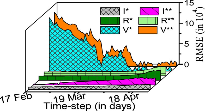
Case-1: RMSE based performance comparison between $SEIRRPV$ and $SIRV$ model, represented with $\ast$, and $\ast \ast$, respectively.

Table 2.

Average $\text{\%}$ RMSE comparison of the $SEIRRPV$ and $SIRV$ model using real-data.

Epidemic model	I	R	P	V
$SEIRRPV$	2.09	2.78	19.7	29.20
$SIRV$	2.60	2.60	$na{n}^{†}$	29.42

$na{n}^{†}$: $\text{\%}$RMSE does not exist for the given compartment.

6.2. Case-2: Comparison with $SIR$ family models

In the above discussions, we limited the comparison of the proposed $SEIRRPV$ model with the $SIRV$ model, as the two models include the vaccinated population in common. We now extend the comparison of the proposed $SEIRRPV$ model with all famous existing models under the $SIR$ family, including the $SIR$, $SIRP$, $SIRV$, $SEIRP$, and $SEIRRP$ models. In this regard, we compare the percentage RMSEs for all models in Table 3. The table concludes an improved accuracy of the proposed $SEIRRPV$ model in comparison to the existing models. To ensure that the estimation errors of the proposed $SEIRRPV$ model for different compartmental populations are within acceptable ranges, we plot the RMSEs of compartmental populations obtained using the proposed $SEIRRPV$ model in Fig. 4.

Table 3.

$\text{\%}$RMSE for different models with 1000 Monte-Carlo simulations.

Model	S	E	I	Re	R	P	V
$SIR$	10.57	$na{n}^{†}$	1.607	$na{n}^{†}$	0.0041	$na{n}^{†}$	$na{n}^{†}$
$SIRP$	11.06	$na{n}^{†}$	1.974	$na{n}^{†}$	0.0901	0.0131	$na{n}^{†}$
$SIRV$	5.359	$na{n}^{†}$	2.246	$na{n}^{†}$	0.0289	$na{n}^{†}$	0.00015
$SEIRP$	45.19	60.57	10.31	$na{n}^{†}$	0.0901	0.0131	$na{n}^{†}$
$SEIRRP$	4.15	3.535	0.0765	1.996	0.00017	0.00017	$na{n}^{†}$
$SEIRRPV$	0.0020	0.0022	0.0011	0.0004	0.00001	0.00001	0.00002

$na{n}^{†}$: $\text{\%}$ RMSE does not exist for the given compartment.

Fig. 4.

Case-2: RMSE of different compartments by $SEIRRPV$ model.

For a comprehensive analysis of the pandemic’s persistence, all parameters corresponding to the basic reproduction number have been analyzed for sensitivity. In this regard, we implemented Eqs. (16), and (17) in Eq. (18) to compute the sensitivity index $\mathcal{S}$ for different epidemic parameters.

The Table 4 shows the sensitivity of the epidemic parameters, such as ${\alpha }_e$, $\alpha$, $\beta$, $\mu$, $\kappa$, $\rho$, $\nu$ and $\Omega$ on the epidemic. Sensitive analysis shows that the most important factor in containing the epidemic is vaccination rate, followed by infection rate, which shows no symptoms and recovery rate. The least sensitive parameter is incubation rate. Positive sensitivity indicates that increases in relevant parameters lead to increases in ${ℛ}_0$, and vice versa. Lower ${\alpha }_e$ and higher $\Omega$ are necessary constraints for lower ${ℛ}_0$ values. As a result of the sensitivity analysis, vaccine rate appears to be more important than the following different nPIs.

Table 4.

Sensitive index for different epidemic parameters.

Parameter	${\alpha }_e$	$\alpha$	$\beta$	$\mu$	$\kappa$	$\rho$	$\nu$	$\Omega$
$\mathcal{S}$	1.00	0.784	−0.98	−0.63	0.11	−0.28	0.79	−4.27

7. Discussion

Covid-19 pandemic caused by SARS-COV-2 started in Wuhan city of China and jolted the entire world within a few months. Its uniqueness is not only its speed of transmission but also life-threatening. In this article, we estimate the dynamics of the covid-19 from the noisy process and measurement model. Process noise is due to various real-life complex constraints involved in it. So accurate information about disease transmission is imperative to strategize correctly. Considering new developments in vaccination, we focus on the proposed $SEIRRPV$ epidemic model to estimate the susceptible, exposed, infected, recovered from exposed, recovered from infected, and passed away people during this pandemic. In this paper, we observed the positive impact of various nPIs, such as social distancing, social awareness, and cleanliness, on the covid-19 pandemic. In addition to this, we observed a rapid decline in the infected population by improving healthcare infrastructure and increasing the mass vaccination drive, as shown in Table 4. We compared the estimation performance of the proposed $SEIRRPV$ model with the existing $SIRV$ model using the real-data of Delhi and compared it with the existing $SIRV$ model using CKF-based method. Fig. 2, Fig. 3 and Table 2 validated that the proposed $SEIRRPV$ has considerably higher estimation accuracy in comparison to the existing $SIRV$ models.

The monitoring and analysis of covid-19 spread using the epidemic models, like the proposed $SEIRRPV$ model, give an edge in formulating appropriate administrative strategies for its control. However, for efficient control of its spread, the public awareness is also equally important, and the public must take care of other measures, like social distancing, use of face-masks, non-pharmaceutical interventions, hand sanitization, etc., seriously. In spreading such awarenesses, the role of print and electronic media has been appreciable and we may have similar expectations from the media in the future. It has been observed that the spread of the first wave of covid-19 (approximately between April to July months of 2020) was relatively slower in India when the people awareness was considered to be at its best. However, the spread was severely faster in the second wave, when the media reports were frequently highlighting a lack of precautions from the public side.

8. Conclusion

An advanced $SIR$ epidemic model named $SEIRRPV$ with the required mathematical analysis is presented in this paper. We present uniqueness, positivity, boundedness, and stability analysis (local and global) for both infection-free and endemic conditions. Epidemic model parameters functionalities are computed from their sensitivity indices. A novel CKF technique is implemented on the proposed epidemic model to dynamically estimate the compartments population. We implemented the proposed model to estimate the disease transmission in Delhi, between 17 January 2021 to 26 April 2021. The simulation study period is important because it witnessed its second wave from March and stretched up to June of 2021. Through simulation-based analysis, we conclude that the proposed $SEIRRPV$ has better performance and also provides additional information to policy-makers about the people who are infected but non-infectious, improving the overall efficiency of the model. However, proposed algorithm does not give information about the evolution of new variants of covid-19, which may stimulate further research. We present a comparative analysis of $SIR$ family’s different epidemic models. Additionally, we validate the proposed $SEIRRPV$ model provides more accurate information to the policy-maker to implement the social and clinical strategy with minimal economic loss. Table 3 and Table 4, respectively, are the estimation accuracy of the proposed epidemic model and sensitivity indices for different epidemic parameters. It concludes that by improving healthcare infrastructure and increasing the mass vaccination drive, epidemic outbreaks can be contained, i.e., ${ℛ}_0$ brought below one. It is possible to extend this research to the dynamic estimation of pandemics with incomplete information and irregular data.

CRediT authorship contribution statement

Sumanta Kumar Nanda: Conceived and designed the analysis, Collected the data, Contributed data or analysis tools, Performed the analysis, Wrote the paper. Guddu Kumar: Contributed data or analysis tools, Performed the analysis, Wrote the paper. Vimal Bhatia: Conceived and designed the analysis, Contributed data or analysis tools, Wrote the paper, Editing & organization of the manuscript. Abhinoy Kumar Singh: Conceived & designed the analysis, Performed the analysis, Wrote the paper, Editing & reorganization of the manuscript.

Declaration of Competing Interest

The authors declare that they have no known competing financial interests or personal relationships that could have appeared to influence the work reported in this paper.

Appendix A. Supplementary data

The following is the Supplementary material related to this article. Proof of Theorem 4.6, 4.8-4.10 are presented in suppymentary material.

MMC S1

.

Data availability

Data will be made available on request.

References

- 1.Cascella M., Rajnik M., Cuomo, et al. Features, evaluation and treatment coronavirus covid-19. Statpearls [Internet] 2020 [PubMed] [Google Scholar]
- 2.Zhang T., Wu Q., Zhang Z. Probable pangolin origin of SARS-CoV-2 associated with the covid-19 outbreak. Curr. Biol. 2020;30(7):1346–1351. doi: 10.1016/j.cub.2020.03.022. [DOI] [PMC free article] [PubMed] [Google Scholar]
- 3.MultiMedia LLC T. 2021. Covid-19 coronavirus pandemic. URL https://www.worldometers.info/coronavirus/ [Google Scholar]
- 4.Mygov T. 2021. Covid-19 coronavirus pandemic. URL https://www.mygov.in/covid-19/?cbps=1/ [Google Scholar]
- 5.Suthar S., Das S., Nagpure Z., et al. Epidemiology and diagnosis, environmental resources quality and socio-economic perspectives for COVID-19 pandemic. J. Environ. Manag. 2021;280 doi: 10.1016/j.jenvman.2020.111700. [DOI] [PMC free article] [PubMed] [Google Scholar]
- 6.Chaudhary P.K., Pachori R.B. FBSED based automatic diagnosis of covid-19 using X-ray and CT images. Comput. Biol. Med. 2021;134 doi: 10.1016/j.compbiomed.2021.104454. [DOI] [PMC free article] [PubMed] [Google Scholar]
- 7.Bhattacharyya A., Bhaik D., et al. A deep learning based approach for automatic detection of COVID-19 cases using chest X-ray images. Biomed. Sig. Proc. Cont. 2022;71 doi: 10.1016/j.bspc.2021.103182. [DOI] [PMC free article] [PubMed] [Google Scholar]
- 8.Di Giamberardino P., Iacoviello D. Evaluation of the effect of different policies in the containment of epidemic spreads for the covid-19 case. Biomed. Sig. Proc. Cont. 2021;65:102325. doi: 10.1016/j.bspc.2020.102325. [DOI] [PMC free article] [PubMed] [Google Scholar]
- 9.Briat C., Verriest E.I. A new delay-SIR model for pulse vaccination. Biomed. Sig. Proc. Cont. 2009;4(4):272–277. [Google Scholar]
- 10.Treesatayapun C. Epidemic model dynamics and fuzzy neural-network optimal control with impulsive traveling and migrating: Case study of covid-19 vaccination. Biomed. Sig. Proc. Cont. 2022;71 doi: 10.1016/j.bspc.2021.103227. [DOI] [PMC free article] [PubMed] [Google Scholar]
- 11.Bhatia V., Mitra R. Signal processing based predictor for covid-19 cases. ResearchGate. 2020 doi: 10.13140/RG.2.2.23431.55201. [DOI] [Google Scholar]
- 12.Lahrouz A., Omari L., et al. Global analysis of a deterministic and stochastic nonlinear SIRS epidemic model. Nonlinear Anal.: Model Control. 2011;16(1):59–76. [Google Scholar]
- 13.Gatto M., Bertuzzo E., et al. Spread and dynamics of the covid-19 epidemic in Italy: Effects of emergency containment measures. Proc. Natl. Acad. Sci. 2020;117(19):10484–10491. doi: 10.1073/pnas.2004978117. [DOI] [PMC free article] [PubMed] [Google Scholar]
- 14.Kabir K.A., Kuga K., Tanimoto J. Analysis of SIR epidemic model with information spreading of awareness. Chaos Solitons Fractals. 2019;119:118–125. [Google Scholar]
- 15.Kermack W.O., McKendrick A.G. A contribution to the mathematical theory of epidemics. Proc. R. Soc. Lond. Ser. A Math. Phys. 1927;115(772):700–721. [Google Scholar]
- 16.Hasan A., Susanto H., et al. A new estimation method for covid-19 time-varying reproduction number using active cases. Sci. Rep. 2022;12(1):1–9. doi: 10.1038/s41598-022-10723-w. [DOI] [PMC free article] [PubMed] [Google Scholar]
- 17.Islam M.S., Hoque M.E., Amin M.R. Integration of Kalman filter in the epidemiological model: a robust approach to predict covid-19 outbreak in Bangladesh. Internat. J. Modern Phys. C. 2021;32(08) [Google Scholar]
- 18.Bootsma M.C., Ferguson N.M. The effect of public health measures on the 1918 Influenza pandemic in US cities. Proc. Natl. Acad. Sci. 2007;104(18):7588–7593. doi: 10.1073/pnas.0611071104. [DOI] [PMC free article] [PubMed] [Google Scholar]
- 19.Sidi Ammi M., Tahiri M. Analysis of Infectious Disease Problems (Covid-19) and their Global Impact. Springer; 2021. Study of transmission dynamics of covid-19 virus using fractional model: case of Morocco; pp. 617–627. [Google Scholar]
- 20.Sameni R. 2020. Mathematical modeling of epidemic diseases; a case study of the covid-19 coronavirus. arXiv preprint arXiv:2003.11371. [Google Scholar]
- 21.Yang W., Sun C., Arino J. Global analysis for a general epidemiological model with vaccination and varying population. J. Math. Anal. Appl. 2010;372(1):208–223. [Google Scholar]
- 22.Parolini N., Ardenghi G., Quarteroni A., et al. Modelling the COVID-19 epidemic and the vaccination campaign in Italy by the SUIHTER model. Infect. Dis. Model. 2022;7(2):45–63. doi: 10.1016/j.idm.2022.03.002. [DOI] [PMC free article] [PubMed] [Google Scholar]
- 23.Song J., Xie H., Gao B., Zhong Y., Gu C., Choi K.-S. Maximum likelihood-based extended Kalman filter for covid-19 prediction. Chaos Solitons Fractals. 2021;146 doi: 10.1016/j.chaos.2021.110922. [DOI] [PMC free article] [PubMed] [Google Scholar]
- 24.Zhu X., Gao B., Zhong Y., et al. Extended Kalman filter based on stochastic epidemiological model for covid-19 modelling. Comput. Biol. Med. 2021;137:104810. doi: 10.1016/j.compbiomed.2021.104810. [DOI] [PMC free article] [PubMed] [Google Scholar]
- 25.Giordano G., Colaneri M., Di Filippo A., et al. Modeling vaccination rollouts, SARS-CoV-2 variants and the requirement for non-pharmaceutical interventions in Italy. Nature Med. 2021;27(6):993–998. doi: 10.1038/s41591-021-01334-5. [DOI] [PMC free article] [PubMed] [Google Scholar]
- 26.Ferguson N.M., Donnelly C.A., Anderson R.M. The foot-and-mouth epidemic in great britain: pattern of spread and impact of interventions. Sci. J. 2001;292(5519):1155–1160. doi: 10.1126/science.1061020. [DOI] [PubMed] [Google Scholar]
- 27.Moore S., Hill E.M., Tildesley M.J., Dyson L., Keeling M.J. Vaccination and non-pharmaceutical interventions for COVID-19: a mathematical modelling study. Lancet Infect. Dis. 2021;21(6):793–802. doi: 10.1016/S1473-3099(21)00143-2. [DOI] [PMC free article] [PubMed] [Google Scholar]
- 28.Trawicki M.B. Deterministic SEIRs epidemic model for modeling vital dynamics, vaccinations, and temporary immunity. Math. 2017;5(1):7. [Google Scholar]
- 29.Arino J., Van Den Driessche P. Positive Systems. Springer; 2003. The basic reproduction number in a multi-city compartmental epidemic model; pp. 135–142. [Google Scholar]
- 30.Golechha M. Covid-19 containment in Asia’s largest Urban Slum Dharavi-Mumbai, India: Lessons for policy-makers globally. J. Urban Health. 2020;97(6):796–801. doi: 10.1007/s11524-020-00474-2. [DOI] [PMC free article] [PubMed] [Google Scholar]
- 31.Wheatley A.K., Juno P., et al. Evolution of immune responses to SARS-CoV-2 in mild-moderate covid-19. Nat. Comm. 2021;12(1):1–11. doi: 10.1038/s41467-021-21444-5. [DOI] [PMC free article] [PubMed] [Google Scholar]
- 32.Arevalo-Rodriguez I., Buitrago P., et al. False-negative results of initial RT-PCR assays for covid-19: a systematic review. PLoS One. 2020;15(12):E0242958. doi: 10.1371/journal.pone.0242958. [DOI] [PMC free article] [PubMed] [Google Scholar]
- 33.Singh U.K., Singh A.K., et al. EKF and UKF based estimators for radar system. Front. Sig. Proc. 2021;1:5. [Google Scholar]
- 34.Oke M., Ogunmiloro O., et al. Mathematical modeling and stability analysis of a SIRV epidemic model with non-linear force of infection and treatment. Commun. Math. Appl. 2019;10(4):717–731. [Google Scholar]
- 35.Khajanchi S., Bera S., Roy T.K. Mathematical analysis of the global dynamics of a HTLV-I infection model, considering the role of cytotoxic T-lymphocytes. Math. Comput. Simul. 2021;180:354–378. [Google Scholar]
- 36.Bera S., Khajanchi S., Roy T.K. Dynamics of an HTLV-I infection model with delayed CTLs immune response. Appl. Math. Comput. 2022;430 [Google Scholar]
- 37.Ottaviano S., Sensi M., Sottile S. Global stability of SAIRS epidemic models. Nonlinear Anal. RWA. 2022;65 [Google Scholar]
- 38.Arasaratnam I., Haykin S., Hurd T.R. Cubature Kalman filtering for continuous-discrete systems: theory and simulations. IEEE Trans. Signal Proces. 2010;58(10):4977–4993. [Google Scholar]
- 39.Arasaratnam I., Haykin S. Cubature Kalman filters. IEEE Trans. Automat. Control. 2009;54(6):1254–1269. [Google Scholar]
- 40.Nanda S.K., Bhatia V., Singh A.K. Performance analysis of Cubature rule based Kalman filter for target tracking. 2020 IEEE 17th India Counc. Int. Conf.; INDICON; IEEE; 2020. pp. 1–6. [Google Scholar]
- 41.Särkkä S., Sarmavuori J. Gaussian filtering and smoothing for continuous-discrete dynamic systems. Signal Proces. 2013;93(2):500–510. [Google Scholar]
- 42.Bhaumik S., Date P. CRC Press; 2019. Nonlinear Estimation: Methods and Applications with Deterministic Sample Points. [Google Scholar]
- 43.Singh A.K., Bhaumik S. Higher degree cubature quadrature Kalman filter. Int. J. Cont. Autom. Syst. 2015;13(5):1097–1105. [Google Scholar]
- 44.Stroud A. Approximate Calculation of Multiple Integrals. Prentice-Hall, Inc.; Englewood Cliffs, NJ: 1971. (Prentice-Hall Ser. in Auto. Comp.). [Google Scholar]
- 45.Bhaumik S. Cubature quadrature Kalman filter. IET Sig. Proc. 2013;7(7):533–541. [Google Scholar]
- 46.Li S., Xu B., et al. Improved maximum correntropy cubature Kalman filter for cooperative localization. IEEE Sens. J. 2020;20(22):13585–13595. [Google Scholar]
Associated Data
This section collects any data citations, data availability statements, or supplementary materials included in this article.
Supplementary Materials
.
Data Availability Statement