Adaptive lasso for the Cox regression with interval censored and possibly left truncated data

Abstract

We propose a penalized variable selection method for the Cox proportional hazards model with interval censored data. It conducts a penalized nonparametric maximum likelihood estimation with an adaptive lasso penalty, which can be implemented through a penalized EM algorithm. The method is proven to enjoy the desirable oracle property. We also extend the method to left truncated and interval censored data. Our simulation studies show that the method possesses the oracle property in samples of modest sizes and outperforms available existing approaches in many of the operating characteristics. An application to a dental caries data set illustrates the method’s utility.

1. Introduction

In biomedical and epidemiological studies, a large number of potential predictors are often collected with the goal of evaluating their effects on a given phenotypic endpoint. For example, the Detroit Dental Health Project (DDHP) collected a wide variety of hypothesized oral health factors covering parenting, diet intake, health behaviors, dental care, social and physical environments, etc., aiming to identify the predictors of early childhood caries in low-income African-American children. Guided by the Fisher-Owens et al.’s¹ conceptual model, Ismail et al.² compiled from the DDHP data a list of over thirty possible predictors for caries progression, and tested their associations with the increment of decayed, filled and missing tooth surfaces between study waves.

Regression modeling is a standard practice to study jointly the effects of multiple predictors on a response. When the number of candidate predictors is large, building a regression model including all of them is undesirable because it has low prediction accuracy and is hard to interpret (Hastie et al.³, section 3.3). For these reasons, variable selection has become an important focus in regression modeling. There have been many statistical methods on variable selection. Among them, a popular class of methods is variable selection via regularization, also known as penalized variable selection. This class of methods has the key advantage of simultaneously selecting important variables and estimating their effects on the outcome. Popular penalized variable selection methods include the lasso,⁴ the smoothly clipped absolute deviation⁵ (SCAD), and the adaptive lasso.⁶ The last two methods enjoy the so-called oracle property: when the sample size is large, they build the regression model as if they knew which of the variables are important. Most of the existing penalized variable selection methods were proposed for linear or generalized linear models, where the outcome is fully observed. There are some methods for censored time-to-event responses. For instance, lasso, SCAD, and adaptive lasso have been extended to the Cox model for right censored data by Tibshirani,⁷ Fan and Li,⁸ and Zhang and Lu,⁹ respectively.

Interval censored time-to-event outcomes arise widely from cohort studies of chronic disease progression, where a subject’s disease status is assessed periodically and thus the time to disease onset is known up to lying between two clinical exams. For instance, in the Detroit Dental Health Project, age of onset of dental caries is interval censored, since the participants’ caries status was assessed periodically every two to three years in the study. As an another example, the Bangkok Metropolitan Administration injecting drug users cohort study¹⁰ examined the subjects for HIV-1 sero-conversion approximately every four months, leading to interval censored time to HIV-1 infection.

Regression analysis for interval censored data has been studied extensively. See Section 5 of Zhang and Sun¹¹ for a review of the literature prior to 2010. Rigorous semiparameric regression methods for mixed case interval censored data,¹² which is the most general type, were developed more recently. Zhang et al.¹³ proposed a sieve maximum likelihood approach for the Cox regression with such data and established its asymptotic properties. Zeng et al.¹⁴ developed a nonparametric maximum likelihood procedure and associated asymptotic theory for a class of semiparametric transformation models.

Despite the extensive literature on regression analysis for interval censored data, variable selection methods for such outcomes are scarce. To the best of our knowledge, there are only three published works^15–17 on penalized variable selection for interval censored data. Wu and Cook¹⁵ assume a proportional hazards model with a piecewise constant baseline hazard function, and perform the variable selection through penalized likelihood estimation with a lasso, SCAD, or adaptive lasso penalty. Although the underlying idea seems quite intuitive, these authors did not provide a careful study of the asymptotic property of the method, and more importantly used a marginal-quantile-based approach to specify the number and location of break points for the piecewise constant baseline hazard function, which is ad hoc. Scolas et al.¹⁶ considered variable selection for interval censored data with a cure fraction and assumed a parametric accelerated failure time mixture cure model. They performed the variable selection via penalized likelihood estimation with double adaptive lasso penalties. Like Wu and Cook¹⁵ and Scolas et al.¹⁶ did not study the asymptotic property of their procedure. Zhao et al.¹⁷ in a recently accepted paper, performed the variable selection for the Cox model with interval censored data through an iteratively reweighted Ridge regression. This approach has two thresholding parameters to tune and uses a sieve estimator for the baseline hazard, which does not have a closed-form updating formula. Hence, it is computationally demanding. Although the article has a proof of oracle property, the simulations therein did not assess the asymptotic normality of the estimators of non-zero regression coefficients.

In this paper, we propose another penalized variable selection method for the Cox proportional hazards model with interval censored data. Unlike Wu and Cook¹⁵ and Zhao et al.,¹⁷ our method avoids approximating the baseline hazard by piecewise constant function, other splines or any polynomial. Instead, it performs the variable selection via a penalized nonparametric maximum likelihood estimation (PNPMLE) with an adaptive lasso penalty. We carefully characterize the support of the PNPMLE of cumulative baseline hazard based on the work of Alioum and Commenges,¹⁸ and develop a penalized EM algorithm, similar in spirit to the EM algorithms in Wang et al.¹⁹ and Zeng et al.,¹⁴ to carry out the penalized nonparametric maximum likelihood estimation. An advantage of our algorithm over Wu and Cook’s¹⁵ and Zhao et al.’s¹⁷ is that the PNPMLE of the baseline hazard has a closed-form updating formula, enhancing the stability and speed of the penalized estimation. We show that our method enjoys the oracle property through both mathematical proof and numerical experiments. We also provide an explicit formula to estimate the covariance matrix of the penalized estimator, which was not provided by Wu and Cook¹⁵ and Zhao et al.,¹⁷ and demonstrate its accuracy in simulations. In addition, we extend the method to left truncated and interval censored data, which has application to longitudinal studies of chronic disease progression where participants are disease-free at enrollment. To the best of our knowledge, this is the first penalized variable selection method for left truncated and interval censored data.

The rest of the article is organized as follows. In Section 2, we describe the algorithm of the penalized variable selection method, a procedure for tuning the penalty parameter, and the approach to estimate the covariance matrix of the penalized estimator. In Section 3, we establish the oracle property of our method, with the proof relegated to a Web Appendix. The extension to left truncated and interval censored data is elaborated in Section 4. Section 5 presents some numerical experiments to evaluate the finite-sample performance of the methods, followed by an application to the DDHP data to identify predictors for age of caries onset in Section 6. We conclude the article by discussing several future research directions.

2. Methodology

2.1. Data and model

We consider a random sample of n independent subjects. Let T_i and Z_i, respectively, denote the time-to-event of interest and a d-dimensional vector of covariates for subject i (i = 1, …, n). We study how to select significant covariates among Z_i for the time-to-event outcome T_i in the situation where T_i is subject to mixed case interval censoring.¹² Denote the sequence of inspection times for subject i by ${\overrightarrow{V}}_i={\left(V_{i1},\dots ,V_{i{K}_i}\right)}^T$. Define Δ_ik = I(V_i,k−1 < T_i ≤ V_ik) (k = 1, …, K_i) with V_i0 = 0, and ${\overrightarrow{\Delta }}_i={\left({\Delta }_{i1},\dots ,{\Delta }_{i{K}_i}\right)}^T$. Then the observed data consist of ${\left\{{𝒪}_i=\left({\overrightarrow{V}}_i,{\overrightarrow{\Delta }}_i,{\mathbf{\text{Z}}}_i\right)\right\}}_{i=1}^n$.

We assume that the inspection process is independent of the time to event given the covariates, i.e. $T_i\perp \left({\overrightarrow{V}}_i,K_i\right)\mid {\mathbf{\text{Z}}}_i$. We also assume that the conditional distribution of T_i given Z_i satisfies the Cox proportional hazards model

$$\lambda \left(t\mid {\text{Z}}_i\right)=\lambda (t)\text{exp}\left({\mathit{\beta }}^T{\text{Z}}_i\right)$$ (1)

where λ(t|Z_i) ≡ lim_Δt→0+ pr(t ≤ T_i < t + Δt|T_i ≥ t, Z_i)/Δt, λ(t) is an unspecified baseline hazard function, and β is a vector of unknown regression parameters.

2.2. Variable selection

We conduct the variable selection via a semiparametric adaptive lasso estimation. Let L_i and R_i denote, respectively, the last inspection time before T_i and the first inspection time after T_i. Set L_i = 0 if T_i is smaller than V_i1 and R_i = ∞ if T_i is larger than $V_{i{K}_i}$, i.e. T_i is right censored. Under the Cox model (1) and the mixed case interval censoring, the logarithm of the observed-data likelihood is

$$l_n(\mathit{\beta },\Lambda )=\sum _{i=1}^n\text{log}\left[\text{exp}\left\{-\Lambda \left(L_i\right)\text{exp}\left({\mathit{\beta }}^T{\text{Z}}_i\right)\right\}-\text{exp}\left\{-\Lambda \left(R_i\right)\text{exp}\left({\mathit{\beta }}^T{\text{Z}}_i\right)\right\}\right]$$ (2)

where $\Lambda (t)={\int }_0^t\lambda (s)\text{d}s$ and the convention, exp{−Λ(∞) exp(β^TZ_i)} = 0, is used. The semiparametric adaptive lasso estimation is

$$\underset{\mathit{\beta },\Lambda }{\text{max}}\left\{l_n(\mathit{\beta },\Lambda )-n\theta \sum _{j=1}^d\left|{\beta }_j\right|/\left|{\tilde{\beta }}_j\right|\right\}$$ (3)

where $\tilde{\mathit{\beta }}\equiv {\left({\tilde{\beta }}_1,\dots ,{\tilde{\beta }}_d\right)}^T$ is the unpenalized nonparametric maximum likelihood estimator for β, which can be obtained using the EM algorithm introduced below but without penalty, θ is a thresholding parameter whose selection is discussed later, and the maximization with respect to Λ is over the space of nondecreasing nonnegative functions. We denote the estimator from equation (3) by $(\widehat{\mathit{\beta }},\widehat{\Lambda })$.

The penalty in equation (3) does not involve Λ. Thus the support set over which $\widehat{\Lambda }(\cdot )$ increases is the same as that of the unpenalized nonparametric maximum likelihood estimator (NPMLE) for Λ, which was characterized by Alioum and Commenges.¹⁸ Specifically, the estimator $\widehat{\Lambda }$ increases only on so-called maximal intersections: intervals of the form (l, u] where $l\in {\left\{L_i\right\}}_{i=1}^n$, $u\in {\left\{R_i\right\}}_{i=1}^n$ and there is no L_i or R_i in (l, u). Additionally, $\widehat{\Lambda }$ is indifferent to how it increases on the maximal intersections, as only the overall jump sizes over (l, u]’s (u < ∞), $\widehat{\Lambda }(u)-\widehat{\Lambda }(l)$, affect the penalized likelihood in equation (3). Write the maximal intersections with a finite upper endpoint as (l₁, u₁], …, (l_m, u_m]. According to the characterization of $\widehat{\Lambda }$, we can assume, just for the purpose of computing $\widehat{\Lambda }$, that Λ is flat on $\overline{{\cup }_{j=1}^m\left(l_j,u_j\right]}$. Define λ_k = Λ(u_k) − Λ(l_k) (k = 1, …, m). Then the log likelihood l_n(β, Λ) can be written as l_n(β, λ), where λ = (λ₁, …, λ_m)^T, and

$$\begin{gathered} l_n(\mathit{\beta },\mathit{\lambda })=\sum _{i=1}^n\text{log}\left[\text{exp}\left\{-\sum _{u_k\le L_i}{\lambda }_k\text{\hspace{0.17em}exp}\left({\mathit{\beta }}^T{\mathbf{\text{Z}}}_i\right)\right\}-I\left(R_i<\infty \right)\text{exp}\left\{-\sum _{u_k\le R_i}{\lambda }_k\text{\hspace{0.17em}exp}\left({\mathit{\beta }}^T{\mathbf{\text{Z}}}_i\right)\right\}\right] \\ =\sum _{i=1}^n\text{log}\left(\text{exp}\left\{-\sum _{u_k\le L_i}{\lambda }_k\text{\hspace{0.17em}exp}\left({\mathit{\beta }}^T{\mathbf{\text{Z}}}_i\right)\right\}\times {\left[1-\text{exp}\left\{-\sum _{L_i<u_k\le R_i}{\lambda }_k\text{\hspace{0.17em}exp}\left({\mathit{\beta }}^T{\mathbf{\text{Z}}}_i\right)\right\}\right]}^{I\left(R_i<\infty \right)}\right) \end{gathered}$$

Direct maximization of $l_n(\mathit{\beta },\mathit{\lambda })-n\theta {\sum }_{j=1}^d\left|{\beta }_j\right|/\left|{\tilde{\beta }}_j\right|$ is challenging because of no closed-form expression for the maximizer $\widehat{\mathit{\lambda }}$, whose dimension increases with the sample size. In the spirit of Zeng et al.,¹⁴ we propose an EM algorithm for the adaptive lasso estimation as follows. Let W_ik (i = 1, …, n; k = 1, …, m) be independent Poisson random variables with means λ_k exp(β^TZ_i). Define $A_i={\sum }_{u_k\le L_i}{W}_{ik}$ and $B_i=I\left(R_i<\infty \right){\sum }_{L_i<u_k\le R_i}{W}_{ik}$. Consider $\widetilde{𝒪}\equiv \{\left(L_i,R_i,{\mathbf{\text{Z}}}_i,A_i=0\right):1\le i\le n$ and R_i = ∞} ∪ {(L_i, R_i, Z_i, A_i = 0, B_i > 0) : 1 ≤ i ≤ n and R_i < ∞} as an observed data set, where A_i = 0 means that A_i is observed to be zero and B_i > 0 means that B_i is observed to be positive. The log likelihood of $\widetilde{𝒪}$ has the form

$$\begin{gathered} \sum _{i=1}^n\text{log}\left[\left\{\prod _{u_k\le L_i}\text{pr}\left(W_{ik}=0\right)\right\}{\left\{1-\text{pr}\left(\sum _{L_i<u_k\le R_i}{W}_{ik}=0\right)\right\}}^{I\left(R_i<\infty \right)}\right] \\ =\sum _{i=1}^n\text{log}\left(\text{exp}\left\{-\sum _{u_k\le L_i}{\lambda }_k\text{\hspace{0.17em}exp}\left({\mathit{\beta }}^T{\text{Z}}_i\right)\right\}{\left[1-\text{exp}\left\{-\sum _{L_i<u_k\le R_i}{\lambda }_k\text{\hspace{0.17em}exp}\left({\mathit{\beta }}^T{\text{Z}}_i\right)\right\}\right]}^{I\left(R_i<\infty \right)}\right) \end{gathered}$$

which is the same as l_n(β, λ). Therefore, we can maximize $l_n(\mathit{\beta },\mathit{\lambda })-n\theta {\sum }_{j=1}^d\left|{\beta }_j\right|/\left|{\tilde{\beta }}_j\right|$ via an EM algorithm by treating $\left\{W_{ik}:i=1,\dots ,n\text{ and }{u}_k\le R_i^{*}\right\}$, where $R_i^{*}=L_{i}I\left(R_i=\infty \right)+R_{i}I\left(R_i<\infty \right)$, as the complete data corresponding to $\widetilde{𝒪}$.

The complete-data log likelihood is

$$\sum _{i=1}^n\sum _{k=1}^{m}I\left(u_k\le R_i^{*}\right)\left[W_{ik}\text{\hspace{0.17em}log}\left\{{\lambda }_k\text{\hspace{0.17em}exp}\left({\mathit{\beta }}^T{\text{Z}}_i\right)\right\}-{\lambda }_k\text{\hspace{0.17em}exp}\left({\mathit{\beta }}^T{\text{Z}}_i\right)-\text{log\hspace{0.17em}}{W}_{ik}!\right]$$ (4)

At the E-step, we compute, $\widehat{E}\left(W_{ik}\right)$, the conditional means of W_ik’s given the observed data $\widetilde{𝒪}$ and the current parameter updates (β^(s), λ^(s)) (s = 0, 1, …,). For u_k ≤ L_i, Ê(W_ik) = 0 since A_i = 0. For L_i < u_k ≤ R_i with R_i < ∞

$$\begin{gathered} \widehat{E}\left(W_{ik}\right)=E\left(W_{ik}\mid L_i,R_i,{\text{Z}}_i,A_i=0,B_i>0\right) \\ =E\left(W_{ik}\mid \sum _{L_i<u_j\le R_i}{W}_{ij}>0\right) \\ =\frac{{\lambda }_k^{(s)}\text{\hspace{0.17em}exp}\left({\mathit{\beta }}^{(s)T}{\text{Z}}_i\right)}{1-\text{exp}\left\{-{\sum }_{L_i<u_j\le R_i}{\lambda }_j^{(s)}\text{\hspace{0.17em}exp}\left({\mathit{\beta }}^{(s)T}{\text{Z}}_i\right)\right\}} \end{gathered}$$

At the M-step, we first maximize the expected complete-data log likelihood with respect to λ conditioning on β. The maximizer has an analytical expression

$${\lambda }_k^{(s+1)}(\mathit{\beta })\equiv \frac{{\sum }_{i=1}^{n}I\left(u_k\le R_i^{*}\right)\widehat{E}\left(W_{ik}\right)}{{\sum }_{i=1}^{n}I\left(u_k\le R_i^{*}\right)\text{exp}\left({\mathit{\beta }}^T{Z}_i\right)}(k=1,\dots ,m)$$

Plugging ${\lambda }_k={\lambda }_k^{(s+1)}(\mathit{\beta })$ into the conditional expectation of equation (4), we update β by maximizing

$$Q\left(\mathit{\beta },{\mathit{\lambda }}^{(s+1)}(\mathit{\beta })\mid {\mathit{\beta }}^{(s)},{\mathit{\lambda }}^{(s)}\right)-n\theta \sum _{j=1}^d\left|{\beta }_j\right|/\left|{\tilde{\beta }}_j\right|$$

where

$$Q\left(\mathit{\beta },{\mathit{\lambda }}^{(s+1)}(\mathit{\beta })\mid {\mathit{\beta }}^{(s)},{\mathit{\lambda }}^{(s)}\right)=\sum _{i=1}^n\sum _{k=1}^{m}I\left(u_k\le R_i^{*}\right)\widehat{E}\left(W_{ik}\right)\times \left[-\text{log}\left\{\sum _{j=1}^{n}I\left(u_k\le R_j^{*}\right)\text{exp}\left({\mathit{\beta }}^T{\text{Z}}_j\right)\right\}+{\mathit{\beta }}^T{\text{Z}}_i\right]$$

and ${\mathit{\lambda }}^{(s+1)}(\mathit{\beta })={\left({\lambda }_1^{(s+1)}(\mathit{\beta }),\dots ,{\lambda }_m^{(s+1)}(\mathit{\beta })\right)}^T$. To perform this maximization, we approximate −Q(β, λ^(s+1)(β)|β^(s), λ^(s)) by a second-order Taylor expansion around β^(s). It can be written in a quadratic form 2⁻¹(Y − Xβ)^T(Y − Xβ), where X is from the Cholesky decomposition of ${\nabla }^{2}Q\left({\mathit{\beta }}^{(s)}\right)\equiv -{\partial }^{2}Q/{\partial \mathit{\beta }\partial {\mathit{\beta }}^T|}_{\mathit{\beta }={\mathit{\beta }}^{(s)}}$, that is ∇²Q(β^(s)) = X^TX, and Y = (X^T)⁻¹ {∇²Q(β^(s))β^(s) − ∇Q(β^(s)) with $\nabla Q\left({\mathit{\beta }}^{(s)}\right)=-\partial Q/{\partial \mathit{\beta }|}_{\mathit{\beta }={\mathit{\beta }}^{(s)}}$. Then we minimize

$$\frac{1}{2}{(\text{Y}-\text{X}\mathit{\beta })}^T(\text{Y}-\text{X}\mathit{\beta })+n\theta \sum _{j=1}^d\left|{\beta }_j\right|/\left|{\tilde{\beta }}_j\right|$$ (5)

to obtain β^(s+1), using the modified shooting algorithm in Zhang and Lu.⁹ The corresponding update for λ is λ^(s+1) = λ^(s+1) (β^(s+1)).

The EM algorithm stops if the maximum of the absolute differences between the estimates at two successive iterations is smaller than, say 10⁻³. We choose the initial parameter values (β⁽⁰⁾, λ⁽⁰⁾) to be the unpenalized nonparametric maximum likelihood estimator $\left(\tilde{\mathit{\beta }},\tilde{\mathit{\lambda }}\right)$, which can be obtained from the same EM algorithm as the above except that the objective function (5) becomes 2⁻¹(Y − Xβ)^T(Y – Xβ). Note that this unpenalized version of EM algorithm is different from the EM algorithm in Zeng et al.,¹⁴ as their algorithm does not make use of the characterization of the NPMLE for cumulative baseline hazard but estimates its jump sizes at every L_i > 0 and R_i < ∞, which is unnecessary and takes longer.

2.3. Covariance matrix of the adaptive lasso estimator

The estimator $\widehat{\mathit{\beta }}$ obtained from equation (3) is equivalent to the solution of the following penalized profile likelihood estimation

$$\underset{\mathit{\beta }}{\text{max}}\left\{l_{pn}(\mathit{\beta })-n\theta \sum _{j=1}^d\left|{\beta }_j\right|/\left|{\tilde{\beta }}_j\right|\right\}$$ (6)

where l_pn(β) = sup_Λ l_n(β, Λ). Adapting the standard error derivation in Section 4.1 of Lu and Zhang²⁰ to equation (6), the covariance matrix of $\widehat{\mathit{\beta }}$ can be estimated by a sandwich formula

$${\left\{{\nabla }^2{l}_{pn}(\widehat{\mathit{\beta }})+n\theta A(\widehat{\mathit{\beta }})\right\}}^{-1}\Sigma (\widehat{\mathit{\beta }}){\left\{{\nabla }^2{l}_{pn}(\widehat{\mathit{\beta }})+n\theta A(\widehat{\mathit{\beta }})\right\}}^{-1}$$ (7)

where ∇²l_pn(β) is the negative hessian of l_pn(β), $\Sigma (\widehat{\mathit{\beta }})=\left\{{\nabla }^2{l}_{pn}(\widehat{\mathit{\beta }})+n\theta D(\widehat{\mathit{\beta }})\right\}{\left\{{\nabla }^2{l}_{pn}(\widehat{\mathit{\beta }})\right\}}^{-1}\left\{{\nabla }^2{l}_{pn}(\widehat{\mathit{\beta }})+n\theta D(\widehat{\mathit{\beta }})\right\}$, $A(\mathit{\beta })=\text{diag}\left(1/{\beta }_1^2,\dots ,1/{\beta }_d^2\right)$ and $D(\mathit{\beta })=\text{diag}\left(I\left({\beta }_1\ne 0\right)/{\beta }_1^2,\dots ,I\left({\beta }_d\ne 0\right)/{\beta }_d^2\right)$. Here we take the convention 0/0 = 0 and set 1/0 to a very large number, say 10¹⁰. A detailed derivation of equation (7) is given in the Web Appendix.

Since l_pn(β) does not have a closed form, we calculate ${\nabla }^2{l}_{pn}(\widehat{\mathit{\beta }})$ using a second-order numerical difference as in Murphy and van der Vaart²¹ (see the first equation on Page 384), that is

$${\left({\nabla }^2{l}_{pn}(\widehat{\mathit{\beta }})\right)}_{i,j}\approx -\frac{l_{pn}\left(\widehat{\mathit{\beta }}+h_n{e}_i+h_n{e}_j\right)-l_{pn}\left(\widehat{\mathit{\beta }}+h_n{e}_i\right)-l_{pn}\left(\widehat{\mathit{\beta }}+h_n{e}_j\right)+l_{pn}(\widehat{\mathit{\beta }})}{h_n^2}$$ (8)

where e_i is the ith unit vector in ${ℝ}^d$ and h_n = O_p(n^−1/2). The value of l_pn(β) can be evaluated using the EM algorithm in Section 2.2 with β held fixed.

2.4. Thresholding parameter tuning

Like all other penalized variable selection methods, the performance of our adaptive lasso estimator ${\widehat{\mathit{\beta }}}_{\theta }$ depends critically on the choice of the thresholding parameter θ. To select it, we minimize the following Bayesian information criterion

$$\text{BIC}(\theta )=-2l_{pn}\left({\widehat{\mathit{\beta }}}_{\theta }\right)+\left|{\alpha }_{\theta }\right|\text{log}(n)$$ (9)

where ${\alpha }_{\theta }=\left\{j:{\widehat{\mathit{\beta }}}_{\theta ,j}\ne 0\right\}$ is the active set identified by the adaptive lasso estimation with thresholding parameter θ, and |α_θ| is its size. For generalized linear models with a fixed number of covariates, the adaptive lasso with the thresholding parameter selected using _BIC identifies the true model consistently.^22,23 This motivates us to use _BIC to select the thresholding parameter in our variable selection method.

3. Asymptotic properties

We study the asymptotic properties of the adaptive lasso estimator $\widehat{\mathit{\beta }}$ obtained from maximizing the penalized likelihood

$$W_n(\mathit{\beta },\Lambda )=l_n(\mathit{\beta },\Lambda )-n{\theta }_n\sum _{j=1}^d\left|{\beta }_j\right|/\left|{\tilde{\beta }}_j\right|$$ (10)

with respect to β and Λ. Denote the true value of β by ${\mathit{\beta }}_0={\left({\mathit{\beta }}_{10}^T,{\mathit{\beta }}_{20}^T\right)}^T$, where β₁₀ denotes the vector of all q non-zero components (1 ≤ q ≤ d) and β₂₀ the vector of zero components. Write $\widehat{\mathit{\beta }}$ as ${\left({\widehat{\mathit{\beta }}}_1^T,{\widehat{\mathit{\beta }}}_2^T\right)}^T$ accordingly.

We assume the following regularity conditions:

• (C1)The true value β₀ belongs to the interior of a known compact set ℬ. The union of the supports of (V₁, …, V_K) is a finite interval [ζ, τ], where 0 < ζ < τ < ∞. The true value of Λ(·), denoted by Λ₀(·), is strictly increasing and continuously differentiable on [ζ, τ], and 0 < Λ₀(ζ) < Λ₀(τ) < ∞.
• (C2)The covariate vector Z is bounded almost surely.
• (C3)The covariance matrix of Z is positive definite.
• (C4)The number of inspection times, K, is positive almost surely, and E(K) < ∞. Additionally, pr(V_j+1 − V_j ≥ η|Z, K) = 1 (j = 1, …, K − 1) for some positive constant η. Furthermore, the conditional densities of (V_j, V_j+1) given (Z, K), denoted by f_j(s, t|Z, K) (j = 1, …, K − 1), have continuous second-order derivatives with respect to s and t when t − s > η and are continuously differentiable with respect to Z.

(C1) is the regularity condition 1 assumed in Zeng et al.¹⁴ (C2) and (C3) are the special cases of their regularity conditions 2 and 3, respectively. (C4) is almost the same as their regularity condition 4 except that we do not assume pr(V_K = τ|Z, K) to be greater than a positive constant since this assumption is too restrictive and unnecessary for proving the asymptotic properties in Zeng et al.,¹⁴ as discussed by Zeng et al.²⁴ The regularity condition 5 in Zeng et al.¹⁴ automatically holds for the Cox proportional hazards model. (C1)–(C4) ensure the root-n consistency of the unpenalized maximum likelihood estimator $\tilde{\mathit{\beta }}$,¹⁴ which is required for the penalty term in equation (10) to be an adaptive lasso penalty as defined in Zou.⁶ These conditions also ensure that the log profile likelihood l_pn(β) has a quadratic expansion around β₀ (Zeng et al.,¹⁴ Remark A1). Our proofs of the asymptotic properties of $\widehat{\mathit{\beta }}$ rely on it.

The following asymptotic results are obtained under the above regularity conditions. Their proofs are relegated to the Web Appendix.

Theorem 1. If $\sqrt{n}{\theta }_n=O_p(1)$, then $\Vert \widehat{\mathit{\beta }}-{\mathit{\beta }}_0\mid \Vert =O_p\left(n^{-1/2}\right)$.

Theorem 2. If $\sqrt{n}{\theta }_n\to 0$ and nθ_n → ∞, then $\widehat{\mathit{\beta }}$ has the following properties:

1. ${\text{lim}}_{n\to \infty }\text{\hspace{0.17em}pr}\left({\widehat{\mathit{\beta }}}_2=0\right)=1$;

2. $\sqrt{n}\left({\widehat{\mathit{\beta }}}_1-{\mathit{\beta }}_{10}\right)\rightsquigarrow N\left(\mathit{0},{\tilde{I}}_{10}^{-1}\right)$, where Ĩ₁₀ is the upper-left q × q sub-matrix of the efficient Fisher information matrix for β, denoted by Ĩ₀, as given implicitly in Zeng et al.¹⁴

The consistency and sparsity of $\widehat{\mathit{\beta }}$ shown in Theorem 1 and Theorem 2(i), respectively, imply that the adaptive lasso estimator enjoys the selection consistency property, that is, lim_n→∞ pr(𝒜_n = {1, …, q}) = 1 with ${𝒜}_n=\left\{j:{\widehat{\beta }}_j\ne 0\right\}$. Theorem 2(ii) implies that the adaptive lasso estimator for the non-zero regression parameters is semiparametrically efficient as if the unimportant covariates were known. It is more efficient than the unpenalized maximum likelihood estimator ${\tilde{\mathit{\beta }}}_1$, whose covariance matrix is ${\left({\tilde{I}}_0^{-1}\right)}_{11}$, the leading q × q sub-matrix of ${\tilde{I}}_0^{-1}$.

4. Extension to left truncated and interval censored data

In this section, we extend the variable selection method to left truncated and interval censored data. Such data have one additional variable V_i0 (i = 1, …, n), the time to entering the study, to the observed data described in Section 2.1. Left truncation means that the random sample comes from the subpopulation of subjects whose time to event is greater than his/her time to study entry, also called left truncation time. To avoid confusion in understanding the sampling plan, we define T*, $V_0^{*}$ and Z* to be the time to event, left truncation time and covariate vector of a subject from the target population, respectively. Then (T_i, V_i0, Z_i) (i = 1, …, n) are a random sample from the subpopulation of (T*, $V_0^{*}$, Z*) with $T^{*}>V_0^{*}$. To describe the assumption below on the inspection process, we introduce a positive random variable U_k (k = 1, …, K) to represent the time from study entry to the k-th inspection of a sampled subject, where K denotes the random total number of inspections. Hence U_ik = V_ik − V_i0 (i = 1, …, n; k = 1, …, K_i). Define $\overrightarrow{U}={\left(U_1,\dots ,U_K\right)}^T$. We assume that T* is independent of ($V_0^{*}$, K, $\overrightarrow{U}$) given Z* and that the joint distribution of ($V_0^{*}$, K, $\overrightarrow{U}$, Z*) does not involve β and Λ.

Under the above assumptions, the log likelihood of left truncated and interval censored data is, up to an additive constant free of (β, Λ),

$$l_n^{(T)}(\mathit{\beta },\Lambda )=\sum _{i=1}^n\text{\hspace{0.17em}log}\left[\text{exp}\left\{-\left(\Lambda \left(L_i\right)-\Lambda \left(V_{i0}\right)\right)\text{exp}\left({\mathit{\beta }}^T{\text{Z}}_i\right)\right\}-\text{exp}\left\{-\left(\Lambda \left(R_i\right)-\Lambda \left(V_{i0}\right)\right)\text{exp}\left({\mathit{\beta }}^T{\text{Z}}_i\right)\right\}\right]$$ (11)

where the superscript (T) means truncation. We perform the variable selection through the following semiparametric adaptive lasso estimation

$$\underset{\mathit{\beta },\Lambda }{\text{max}}\left\{l_n^{(T)}(\mathit{\beta },\Lambda )-n\theta \sum _{j=1}^d\left|{\beta }_j\right|/\left|{\tilde{\beta }}_j\right|\right\}$$ (12)

where $\tilde{\mathit{\beta }}\equiv {\left({\tilde{\beta }}_1,\dots ,{\tilde{\beta }}_d\right)}^T$ is the unpenalized nonparametric maximum likelihood estimator for β, which can be obtained using the EM algorithm below except no penalty being involved, θ is a thresholding parameter whose selection can follow the method in Section 2.4, and the maximization with respect to Λ is over the space of nondecreasing nonnegative functions. We denote the estimator from equation (12) by $(\widehat{\mathit{\beta }},\widehat{\Lambda })$.

Similar to the case of interval censored data, $\widehat{\Lambda }$ has the same characterization as the unpenalized nonparametric maximum likelihood estimator for Λ, which was given in Alioum and Commenges.¹⁸ Specifically, the estimator $\widehat{\Lambda }$ increases only on intervals of the form (l, u] where $l\in {\left\{L_i\right\}}_{i=1}^n$, $u\in {\left\{R_i,V_{i0}\right\}}_{i=1}^n$ and there is no L_i, R_i or V_i0 in (l, u). Additionally, $\widehat{\Lambda }$ is indifferent to how it increases on those intervals, as only the overall jump sizes over (l, u]’s with l > 0 and u < ∞, $\widehat{\Lambda }(u)-\widehat{\Lambda }(l)$, affect the penalized likelihood in equation (12). Write the intervals (l, u]’s with l > 0 and u < ∞ as (l₁, u₁], …, (l_m, u_m]. According to the characterization of $\widehat{\Lambda }$, we can assume, just for the purpose of computing $\widehat{\Lambda }$, that Λ is flat on $\overline{{\cup }_{j=1}^m\left(l_j,u_j\right]}$. Define λ_k = Λ(u_k) − Λ(l_k) (k = 1, …, m). Then the log likelihood $l_n^{(T)}(\mathit{\beta },\Lambda )$ can be written as $l_n^{(T)}(\mathit{\beta },\mathit{\lambda })$, where λ = (λ₁, …, λ_m)^T, and

$$\begin{gathered} l_n^{(T)}(\mathit{\beta },\mathit{\lambda })=\sum _{i=1}^n\text{\hspace{0.17em}log}\left[\text{exp}\left\{-\sum _{V_{i0}<u_k\le L_i}{\lambda }_k\text{\hspace{0.17em}exp}\left({\mathit{\beta }}^T{\text{Z}}_i\right)\right\}-I\left(R_i<\infty \right)\text{exp}\left\{-\sum _{V_{i0}<u_k\le R_i}{\lambda }_k\text{\hspace{0.17em}exp}\left({\mathit{\beta }}^T{\text{Z}}_i\right)\right\}\right] \\ =\sum _{i=1}^n\text{\hspace{0.17em}log}\left(\text{exp}\left\{-\sum _{V_{i0}<u_k\le L_i}{\lambda }_k\text{\hspace{0.17em}exp}\left({\mathit{\beta }}^T{\text{Z}}_i\right)\right\}\times {\left[1-\text{exp}\left\{-\sum _{L_i<u_k\le R_i}{\lambda }_k\text{\hspace{0.17em}exp}\left({\mathit{\beta }}^T{\text{Z}}_i\right)\right\}\right]}^{I\left(R_i<\infty \right)}\right) \end{gathered}$$

In view of the similarity between $l_n^{(T)}(\mathit{\beta },\mathit{\lambda })$ and l_n(β, λ), the semiparametric adaptive lasso estimation (12) can be performed using the same EM algorithm as for the case of interval censored data except that the indices u_k ≤ L_i are replaced by V_i0 < u_k ≤ L_i throughout the algorithm. The covariance matrix of the resulting estimator can be estimated using the same approach as in Section 2.3.

5. Numerical experiments

To evaluate the finite sample performance of our variable selection methods, we conducted numerical experiments in two cases, one without left truncation and one with it. In the former, we also compare the performance of our method with Wu and Cook’s¹⁵ and Zhang and Lu’s,⁹ for the latter of which the event times were obtained using mid-point imputations. We used the R codes developed by those authors to implement Wu and Cook’s¹⁵ and Zhang and Lu’s⁹ methods. It is worthwhile to also compare our method with Zhao et al.’s¹⁷ in simulations. However, due to the lack of available software implementing their method and the difficulty of implementing by ourselves, we did not make the comparison.

The simulation scenario is the following. For every subject of a sample, a vector of ten covariates is generated from a multivariate normal distribution, Z_i ~ MVN₁₀(0, Σ) where Σ is the covariance matrix whose ij-th element is Σ_ij = 0.5^|i−j|. We set β_j = 0.5 for j = 1, 2, 9, and 10, and β_j = 0 for j = 3, …, 8 in the Cox model, λ(t|Z_i) = λ(t) exp(β^TZ_i). We use the Weibull hazard as the baseline hazard function, λ(t) = κη(ηt)^κ−1 with κ = 1.5 and η = 0.2, which renders P(T_i < 10|Z_i = 0) ≈ 0.95. The number of planned inspections is three, but we allow subjects to miss each of the second and third planned inspections with a 5% chance so that the actual number of inspections could vary across subjects. This mimics the actual follow-up of the DDHP study. In the untruncated case, the inspection times V₁, V₂ and V₃ are generated from V₁ ~ U(3.2, 4.8), V₂ = V₁ + U(1.5, 2.5), and V₃ = V₂ + U(1.5, 2.5). In the truncated case, we generate the left-truncation time V₀ from V₀ = 2.5 + U(0, 4), and the inspection times are obtained from V₁ = V₀ + U(3.2, 4.8), V₂ = V₁ + U(1.5, 2.5) and V₃ = V₂ + U(1.5, 2.5). The proportions of subjects being right-censored are 24.2% in the untruncated case and 29.7% in the truncated case. We considered two sample sizes, 200 and 400. One thousand Monte Carlo samples were generated for each sample size. However, for 247 Monte Carlo samples of size 200 and 210 samples of size 400, Wu and Cook’s¹⁵ method failed to converge for a wide range of thresholding parameter values. We removed these Monte Carlo samples from computing the simulation performance measurements for their method.

Table 1 gives the variable selection percentages of our method, Zhang and Lu’s⁹ method based on mid-point imputation, and Wu and Cook’s¹⁵ method in the untruncated case. Our method’s selection percentages of significant covariates are almost 1 and higher than the other two methods. Our method’s selection percentages of non-significant covariates are less than 8% for n = 200 and less than 5% for n = 400, slightly worse than Zhang and Lu’s⁹ but better than Wu and Cook’s.¹⁵ All the three methods’ variable selection percentages improved with the sample size. Table 2 shows the average numbers of correct and incorrect zero coefficients as well as the mean squared error of the coefficient estimator, ${(\widehat{\beta }-\beta )}^T\Sigma (\widehat{\beta }-\beta )$, where Σ is the population covariance matrix of the covariates. Our method outperforms the other two in terms of the average numbers of incorrect zero coefficients and the mean squared error. Zhang and Lu’s⁹ method has a relatively large mean squared error because of the estimation bias for the non-zero coefficients caused by the mid-point imputation, as shown in Table 3. Our method’s average numbers of correct zero coefficients are only worse than Zhang and Lu’s,⁹ but are still reasonably good. Table 3 gives the mean estimate, the empirical standard error of the estimator, the mean of the standard error estimates, and the coverage of the Normal-based confidence interval for the non-zero coefficients. For the variance estimation of our method and the oracle method, we set h_n = 5n^−1/2. Concurring with the theory, our method performs like the oracle method as the sample size increases. Even in small samples, our variance formula (7) is rather accurate, and our estimators for the non-zero coefficients showed normality, as reflected by the coverage of the Normal-based confidence intervals and the Normal Q-Q plots in Figure 1(a). Zhang and Lu’s⁹ estimators were shown to be biased. This is because of the mid-point imputation. Wu and Cook’s¹⁵ method performs well in terms of bias and empirical variance, but it has convergence issues as mentioned earlier. The standard errors and the coverage of the Normal-based confidence intervals for Wu and Cook’s¹⁵ method were not computed, because the bootstrap, suggested by them for computing the standard errors, experienced convergence issues for some of the bootstrap samples. Figure 1 shows that our regularized estimators for the non-zero coefficients converge to Normal in distribution as the sample size increases.

Table 1.

The variable selection percentages of our method, Zhang and Lu’s⁹ method based on mid-point imputation, and Wu and Cook’s¹⁵ method in the untruncated case.

N	Method	Z 1	Z 2	Z 3	Z 4	Z 5	Z 6	Z 7	Z 8	Z 9	Z 10
200	Ours	0.997	0.993	0.067	0.067	0.069	0.060	0.072	0.066	0.992	0.993
	ZL	0.974	0.963	0.038	0.019	0.032	0.030	0.035	0.035	0.967	0.971
	WC	0.991	0.992	0.121	0.102	0.112	0.086	0.106	0.130	0.987	0.983
400	Ours	1.000	1.000	0.037	0.026	0.042	0.040	0.047	0.033	1.000	1.000
	ZL	0.999	0.998	0.012	0.009	0.008	0.009	0.012	0.008	1.000	0.999
	WC	0.996	0.995	0.113	0.086	0.085	0.090	0.106	0.109	0.996	0.998

Ours: our method; ZL: Zhang and Lu’s⁹ method based on mid-point imputation; WC: Wu and Cook’s¹⁵ method.

Table 2.

Average numbers of correct and incorrect zero coefficients and mean squared errors of the coefficient estimators in the untruncated case.

n	Method	Correct (6)	Incorrect (0)	MSE
200	Ours	5.599	0.025	0.083
	ZL	5.811	0.125	0.297
	WC	5.343	0.048	0.098
400	Ours	5.775	0	0.034
	ZL	5.942	0.004	0.229
	WC	5.411	0.015	0.043

Note: In the parentheses are the ideal numbers of correct and incorrect zero coefficients. MSE: mean squared error; Ours: our method; ZL: Zhang and Lu’s⁹ method based on mid-point imputation; WC: Wu and Cook’s¹⁵ method.

Table 3.

Simulation results on the estimation of the non-zero coefficients in the untruncated case.

	n = 200				n = 400
Coef	Est	CP	SE	SEE	Est	CP	SE	SEE
Oracle
β1 = 0.5	0.531	0.974	0.123	0.137	0.518	0.963	0.085	0.090
β2 = 0.5	0.535	0.972	0.124	0.136	0.516	0.961	0.090	0.089
β9 = 0.5	0.536	0.972	0.127	0.137	0.517	0.953	0.087	0.089
β10=0.5	0.525	0.969	0.124	0.136	0.517	0.961	0.084	0.090
Our method
β1= 0.5	0.481	0.939	0.140	0.139	0.491	0.952	0.091	0.091
β2 = 0.5	0.483	0.948	0.147	0.150	0.488	0.948	0.098	0.098
β9 = 0.5	0.484	0.955	0.148	0.149	0.488	0.947	0.094	0.098
β10=0.5	0.476	0.936	0.142	0.138	0.490	0.937	0.091	0.091
Zhang and Lu’s9
β1 = 0.5	0.298	0.470	0.133	0.097	0.318	0.299	0.089	0.068
β2 = 0.5	0.296	0.493	0.134	0.097	0.314	0.280	0.090	0.068
β9 = 0.5	0.300	0.485	0.135	0.097	0.314	0.285	0.090	0.068
β10 = 0.5	0.295	0.469	0.132	0.097	0.315	0.285	0.086	0.068
Wu and Cook’s15
β1 = 0.5	0.514	–	0.132	–	0.507	–	0.094	–
β2 = 0.5	0.514	–	0.139	–	0.504	–	0.101	–
β9 = 0.5	0.515	–	0.150	–	0.504	–	0.102	–
β10 = 0.5	0.512	–	0.146	–	0.505	–	0.091	–

Note: The standard errors and the coverage of the Normal-based confidence intervals for Wu and Cook’s¹⁵ method were not computed due to the bootstrap, suggested by them for computing the standard errors, experiencing convergence issues for some of the bootstrap samples. Oracle: the unpenalized nonparametric maximum likelihood estimation with only the covariates whose coefficients are non-zero, i.e. Z₁, Z₂, Z₉ and Z₁₀; Coef: regression coefficient; Est: empirical average of the parameter estimator; CP: empirical coverage of the 95% Normal-based confidence interval; SE: empirical standard error of the parameter estimator; SEE: empirical average of the standard error estimator.

Figure 1.

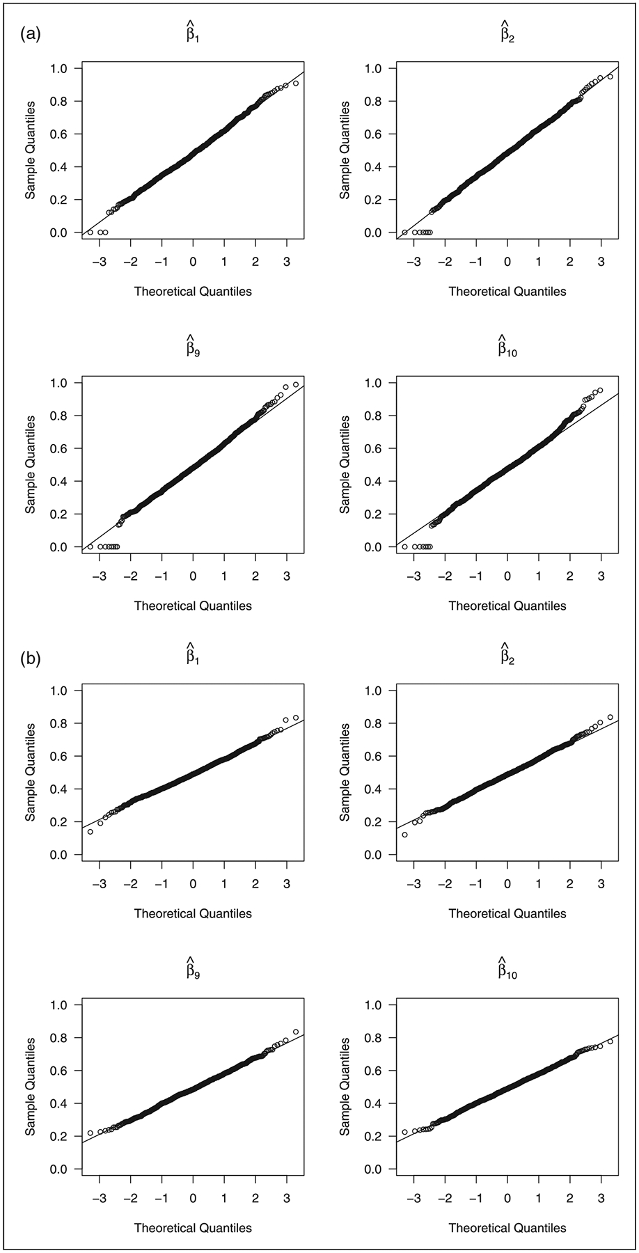
Normal Q–Q plots of the proposed estimators for the non-zero coefficients in the untruncated case. (a) n = 200; (b) n = 400.

The simulation results for the truncated case are in the Web Appendix. In the truncated case, our adaptive lasso method also performed very well in terms of variable selection percentages, average numbers of correct and incorrect zero coefficients, and estimation accuracy of the non-zero coefficients. Figure S1 in the Web Appendix shows that the distributions of our regularized estimators for the non-zero coefficients converge to Normal as the sample size increases. For the variance estimation of our method and the oracle method in the truncated case, we again set h_n = 5n^−1/2.

6. Application

We apply the proposed method to the data of Detroit Dental Health Project. This is a longitudinal study that was designed to understand the oral health of low income African-American children in the city of Detroit. A total of 1021 dyads of children and their caregivers were enrolled in the study. The study collected a broad array of hypothesized determinants of oral health and made tooth-surface-level caries assessments on the participants over three waves from 2003 to 2007. The subjects considered in our analysis are the child participants. At Wave I, the children’s age range is 0–5 years with an average of 2.6. In the analysis, we consider the event of interest to be that a child has any non-cavitated or cavitated lesion in the primary dentition. We use age as the time scale and call the time to event age to caries. According to the study design, each child had one to three inspection times depending on whether he or she missed study visits. So the age to caries is either left censored, interval censored or right censored. The number of children in the analyzed data set is 1020, because one child does not have age-at-inspection information. We study the effects of child-, family- and community-level factors on mouth-level primary dental caries development. A list of variables considered in the analysis are in Table 4. All of them except WATER were picked out from Ismail et al.⁴ by excluding the obviously time-varying predictors therein. These variables’ values at Wave I were used in the analysis, assuming that the time-dependent variables in the list did not change much during the follow-up, which is reasonable to some extent owing to the dichotomization of many of the time-dependent variables.

Table 4.

The candidate covariates considered in the analysis of Detroit Dental Health Project.

Variable name	Variable description
Child-level
GENDER	Gender of child
WEIGHT	Weight-for-age percentile
BRUSHRATE	Brushing frequency during the preceding week (0 for < 7; 1 for ≥ 7)
WIPE	Frequency of wiping teeth of the child (0 = never or rarely; 1 = sometimes or usually)
WATER	Frequency of cleaning teeth of the child with water (0 = never or rarely; 1 = sometimes or usually)
WIC	Participating in WIC (0 = no; 1 = yes)
HEADSTART	Participating in Head Start (0 = no; 1 = yes)
Family-level
OHSE	Caregiver’s score of perception of self-efficacy related to brushing the child’s teeth regularly
KBU	Caregiver’s score of knowledge of bottle use
KCOH	Caregiver’s score of knowledge of children’s oral hygiene
OHF	Caregiver’s belief in oral health fatalism (0 = neutral, disagree, or strongly disagree; 1 = agree or strongly agree)
KITCHEN	Water filter/purifier on kitchen tap (0 = no; 1 = yes)
CESD	Caregiver’s depressive symptoms (0 = absence; 1 = presence)
PARENTSTRESS	Caregiver’s parenting stress score
SUPPORT	Social support received by the caregiver (0 = low; 1 = high)
EDU	Caregiver’s education attainment (0 = less than high school; 1 = high school diploma or more)
EMPLOYMENT	Caregiver’s full-time employment status (0 = no; 1 = yes)
RELIGIOUSNESS	Caregiver’s frequency of attending religious services (0 for less than three times a month; for at least once a week)
Community-level
DENTIST	Number of dentists in the neighborhood
GROCER	Number of grocery stores in the neighborhood
CHURCH	Number of churches in the neighborhood

The data analysis results are shown in Table 5. Six covariates, BRUSHRATE, WIPE, HEADSTART, OHSE, KBU and EDU, were selected into the Cox model by the proposed adaptive lasso approach. All of their effect directions except WIPE’s make common sense. A possible explanation about the positive effect of WIPE could be that the wiping cloth was dirty so that wiping teeth accelerated the caries development. As can be seen from Table 5, the 5%-level two-sided Wald tests for each covariate based on the nonparametric maximum likelihood estimation would pick BRUSHRATE, WIPE, HEADSTART and OHSE as significant covariates, a subset of the covariates selected by the adaptive lasso. This test-based variable selection approach suffers from the multipletesting issue, especially in this case of 21 candidate covariates.

Table 5.

Results of the analysis of Detroit Dental Health Project.

Variable	NPMLE	Adaptive lasso
Child-level
GENDER	−0.037 (0.038)	0 (−)
WEIGHT	−0.028 (0.038)	0 (−)
BRUSHRATE	−0.111 (0.041)	−0.189 (0.084)
WIPE	0.181 (0.040)	0.342 (0.083)
WATER	0.016 (0.040)	0 (−)
WIC	0.036 (0.040)	0 (−)
HEADSTART	−0.117 (0.037)	−0.268 (0.105)
Family-level
OHSE	−0.080 (0.039)	−0.093 (0.052)
KBU	−0.079 (0.043)	−0.040 (0.041)
KCOH	0.040 (0.044)	0 (−)
OHF	0.036 (0.040)	0 (−)
KITCHEN	0.013 (0.037)	0 (−)
CESD	−0.005 (0.040)	0 (−)
PARENTSTRESS	−0.054 (0.042)	0 (−)
SUPPORT	0.032 (0.043)	0 (−)
EDU	−0.069 (0.041)	−0.082 (0.081)
EMPLOYMENT	−0.033 (0.039)	0 (−)
RELIGIOUSNESS	−0.051 (0.042)	0 (−)
Community-level
DENTIST	0.056 (0.050)	0 (−)
GROCER	0.021 (0.050)	0 (−)
CHURCH	−0.043 (0.045)	0 (−)

Note: Standard errors are given in the parentheses. NPMLE: the coefficient estimate from the nonparametric maximum likelihood estimation; Adaptive lasso: the coefficient estimate from the proposed shrinkage method.

7. Discussion

Section 4 actually also provides an unpenalized nonparametric maximum likelihood estimation algorithm for the Cox model with left truncated and interval censored data. The covariance matrix of the corresponding regression coefficient estimator can be estimated using the profile likelihood method.²⁵ These approaches, to the best of our knowledge, are new in the literature. They performed well in finite samples, as seen in Table S3 of the Web Appendix.

The proposed variable selection method can be readily extended to interval censored data with time-dependent covariates whose trajectories are fully observed, e.g., marital status and parity. The asymptotic properties for the extension can be also easily derived based on this paper and Zeng et al.,¹⁴ which considered fully-observed time-dependent covariates. Computationally, it is straightforward to extend our method to other semiparametric transformation models in Zeng et al.¹⁴ and to other penalties like SCAD. The proofs of the corresponding asymptotic theories would be a bit more involved though, since the profile likelihood for other transformation models is a more complex function of regression parameters and SCAD is not a convex penalty. A more interesting and challenging extension is to the high-dimensional setting, i.e. d is comparable to n or even much larger than n. We are working on this problem.

References

- 1.Fisher-Owens SA, Gansky SA, Platt LJ, et al. Influences on children’s oral health: a conceptual model. Pediatrics 2007; 120: e510–e520. [DOI] [PubMed] [Google Scholar]
- 2.Ismail A, Sohn W, Lim S, et al. Predictors of dental caries progression in primary teeth. J Dental Res 2009; 88: 270–275. [DOI] [PMC free article] [PubMed] [Google Scholar]
- 3.Hastie T, Tibshirani R and Friedman J. The elements of statistical learning: data mining, inference and prediction. 2nd ed. Springer, 2009. [Google Scholar]
- 4.Tibshirani R Regression shrinkage and selection via the lasso. J Royal Stat Soc Ser B (Methodological) 1996; 58: 267–288. [Google Scholar]
- 5.Fan J and Li R. Variable selection via nonconcave penalized likelihood and its oracle properties. J Am Stat Assoc 2001; 96: 1348–1360. [Google Scholar]
- 6.Zou H The adaptive lasso and its oracle properties. J Am Stat Assoc 2006; 101: 1418–1429. [Google Scholar]
- 7.Tibshirani R The lasso method for variable selection in the Cox model. Stat Med 1997; 16: 385–395. [DOI] [PubMed] [Google Scholar]
- 8.Fan J and Li R. Variable selection for Cox’s proportional hazards model and frailty model. Annals Stat 2002; 30: 74–99. [Google Scholar]
- 9.Zhang HH and Lu W. Adaptive lasso for Cox’s proportional hazards model. Biometrika 2007; 94: 691–703. [Google Scholar]
- 10.Vanichseni S, Kitayaporn D, Mastro TD, et al. Continued high HIV-1 incidence in a vaccine trial preparatory cohort of injection drug users in Bangkok, Thailand. AIDS 2001; 15: 397–405. [DOI] [PubMed] [Google Scholar]
- 11.Zhang Z and Sun J. Interval censoring. Stat Meth Med Res 2010; 19: 53–70. [DOI] [PMC free article] [PubMed] [Google Scholar]
- 12.Schick A and Yu Q. Consistency of the GMLE with mixed case interval-censored data. Scand J Stat 2000; 27: 45–55. [Google Scholar]
- 13.Zhang Y, Hua L and Huang J. A spline-based semiparametric maximum likelihood estimation method for the Cox model with interval-censored data. Scand J Stat 2010; 37: 338–354. [Google Scholar]
- 14.Zeng D, Mao L and Lin DY. Maximum likelihood estimation for semiparametric transformation models with interval-censored data. Biometrika 2016; 103: 253–271. [DOI] [PMC free article] [PubMed] [Google Scholar]
- 15.Wu Y and Cook RJ. Penalized regression for interval-censored times of disease progression: selection of HLA markers in psoriatic arthritis. Biometrics 2015; 71: 782–791. [DOI] [PubMed] [Google Scholar]
- 16.Scolas S, El Ghouch A, Legrand C, et al. Variable selection in a flexible parametric mixture cure model with interval-censored data. Stat Med 2016; 35: 1210–1225. [DOI] [PMC free article] [PubMed] [Google Scholar]
- 17.Zhao H, Wu Q, Li G, et al. Simultaneous estimation and variable selection for interval-censored data with broken adaptive ridge regression. J Am Stat Assoc. Epub ahead of print 22 April 2019. DOI: 10.1080/01621459.2018.1537922. [DOI] [PMC free article] [PubMed] [Google Scholar]
- 18.Alioum A and Commenges D. A proportional hazards model for arbitrarily censored and truncated data. Biometrics 1996; 52: 512–524. [PubMed] [Google Scholar]
- 19.Wang L, McMahan CS, Hudgens MG, et al. A flexible, computationally efficient method for fitting the proportional hazards model to interval-censored data. Biometrics 2016; 72: 222–231. [DOI] [PMC free article] [PubMed] [Google Scholar]
- 20.Lu W and Zhang HH. Variable selection for proportional odds model. Stat Med 2007; 26: 3771–3781. [DOI] [PubMed] [Google Scholar]
- 21.Murphy SA and van der Vaart AW. Observed information in semi-parametric models. Bernoulli 1999; 5: 381–412. [Google Scholar]
- 22.Zhang Y, Li R and Tsai CL. Regularization parameter selections via generalized information criterion. J Am Stat Assoc 2010; 105: 312–323. [DOI] [PMC free article] [PubMed] [Google Scholar]
- 23.Hui FKC, Warton DI and Foster SD. Tuning parameter selection for the adaptive lasso using ERIC. J Am Stat Assoc 2015; 110: 262–269. [Google Scholar]
- 24.Zeng D, Gao F and Lin DY. Maximum likelihood estimation for semiparametric regression models with multivariate interval-censored data. Biometrika 2017; 104: 505–525. [DOI] [PMC free article] [PubMed] [Google Scholar]
- 25.Murphy SA and van der Vaart AW. On profile likelihood. J Am Stat Assoc 2000; 95: 449–465. [Google Scholar]
Associated Data
This section collects any data citations, data availability statements, or supplementary materials included in this article.