SVision: A deep learning approach to resolve complex structural variants

Abstract

Complex structural variants (CSVs) encompass multiple breakpoints and are often missed or misinterpreted by state-of-the-art variant detection algorithms. We developed SVision, a deep-learning based multi-object recognition framework, to automatically detect and characterize CSVs from long-read data. SVision outperforms current variant callers at identifying internal structure of complex events and revealed 80 high-quality CSVs with 25 distinct structures from an individual genome. SVision directly detects CSVs without pattern matching against a database of known structures, allowing sensitive detection of both common and previously uncharacterized complex rearrangements.

Complex structural variants (CSVs) contain multiple breakpoints and may delete, duplicate, and/or invert multiple segments of DNA in both healthy¹ and disease genomes^{2, 3}, creating events more likely to be deleterious than simple structural variants (SVs)^{4, 5}. Previous short-read based studies detected CSVs via intensive breakpoint analysis, but subsequent manual inspections with complementary data were required to determine CSV internal structures^{1, 6}, hindering CSV study in population-scale. Even though long-reads have greatly facilitated the detection of phased SVs⁷ and somatic SV^{4, 8}, three major issues have impeded their use in CSV detection. Firstly, the model-based inference approach, initially designed for simple SV discovery from short-reads⁹, requires construction of each SV model for fitting aberrant alignment patterns (Extended Data Fig. 1) and prohibits effective discovery of largely unexplored CSV structures^{10, 11}. Secondly, ambiguous alignments at repetitive regions complicate SV discovery, leading to false calls or missing events⁶. Lastly, current subjective definition of CSV types is based on predefined models lacking a unified and computer-interpretable framework, thereby prohibiting cross-study comparison of CSVs.

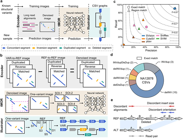
We developed SVision, a method designed to automatically detect and characterize complex variants from long-read data. SVision begins by encoding pairs of sequences, a given read and its counterpart in reference genome, as an image showing sequence similarity and difference adapting variant detection to a multi-object recognition problem amenable to existing deep learning frameworks. SVision is composed of three core components: an encoder that represents the differences and similarities between a variant supporting read and its corresponding segment in the reference genome as a denoised image, a targeted multi-object recognition (tMOR) framework that detects and characterizes CSVs via a convolutional neural network (CNN) in the denoised image, and an illustrator that creates and unifies each detected CSV as a graph representation from the denoised image (Fig. 1a). To generate a denoised image, the encoder first collects aberrant long-read alignments, the so-called variant feature sequence (VAR), and its aligned segment on the reference genome, referring to reference sequence (REF). For a VAR, the encoder identifies matched and unmatched bases, from which the matched and the locally realigned unmatched sequences are combined to create VAR-to-REF and REF-to-REF images (Fig. 1b). Since the repetitive sequences are present in both variant feature and reference sequences, the variant signature can be isolated and accentuated when the reference background is removed. Thus, a denoised image is created for each feature sequence by subtracting REF-to-REF image from its corresponding VAR-to-REF image, which reduces false calls introduced by repeats (Online Methods). In the tMOR step, since a denoised image might contain more than one SV, SVision uses a two-step image segmentation process to first obtain one-variant images, containing the full structure of a SV. Then, SVision defines each location surrounding a breakpoint in the one-variant image as a Segment of Interest (SOI), and SOIs that are collected from a one-variant image are recognized as a single CSV through a pre-trained CNN (Online Methods). The third component of SVision, illustrator, adopts a graph-based approach to depict different CSV structures. A given CSV graph structure and its topologically equivalent events are combined through detection of isomorphic graphs (Online Methods). Additionally, SVision reports the CSV graph in the Reference Graphical Fragment Assembly (rGFA) format introduced by MiniGraph¹² (Online Methods). Finally, SVision clusters similar one-variant images that supports an event and integrates CNN prediction probability of each one-variant image and similarity across one-variant images in a cluster to measure confidence of an event.

Fig. 1 ∣. Workflow and evaluation of SVision detecting complex structural variants.

a, Overview of three modules in SVision. b, Workflow of each module; SOI- segment of interest. c, Performance for calling simulated complex structural variants (CSVs) was evaluated by recall (y-axis), precision (x-axis) and F-score (F, dashed line). d, SVision detected all previously reported and manually curated NA12878 CSVs, all of which passed exact match criteria. e, A misinterpreted complex event from short-read data, which is correctly detected by Svision as simple deletion. This event is surrounded by repeats that introduce two distinct patterns of discordant paired-end mapping, misleading short-read callers to report a CSV.

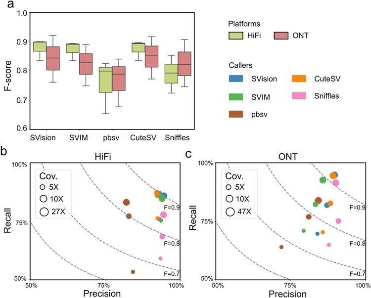
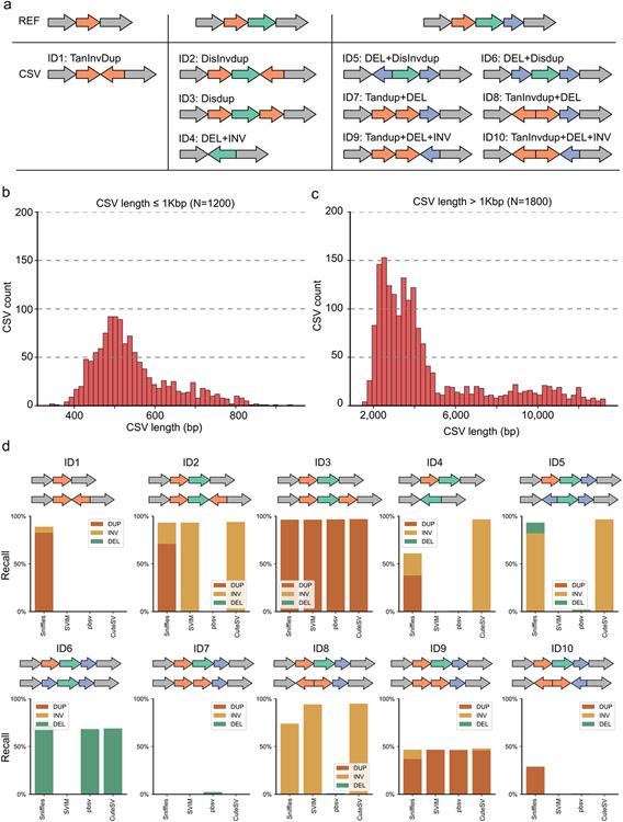
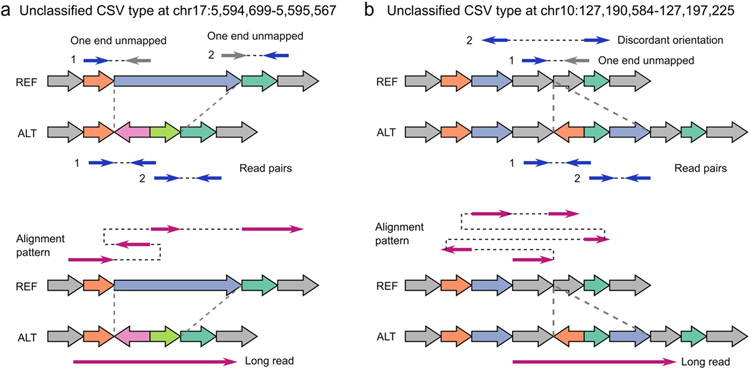
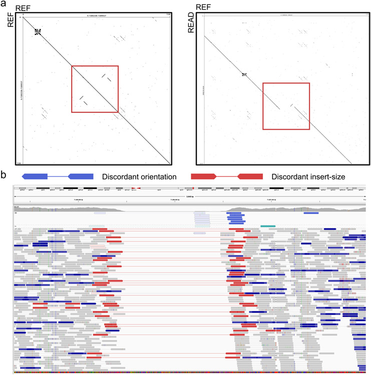
We next explored how well the sequence-to-image coding schema and the CNN model perform across different long-read sequencing platforms for canonical SV detection, where SVision, CuteSV¹³, pbsv, SVIM¹⁴ and Sniffles¹⁰ were applied to the HG002 genome (~27X PacBio HiFi and ~47X Oxford Nanopore, ONT) released by Genome-In-A-Bottle¹⁵. The results showed that SVision outperforms other callers at all different coverages (Supplementary Table S1), where the F-score of SVision ranged from 0.83 to 0.90 for HiFi and from 0.76 to 0.92 for ONT (Extended Data Fig. 2). Furthermore, performance was also assessed on simulated CSVs of 10 types (Extended Data Fig. 3a-c) extracted from the 1000 Genomes Project (1KGP)¹ and a cohort study of autism disorders² (Online Methods). The simulated genome harboring 3,000 CSVs (300 per each of 10 types, Supplementary Table S2) was created on one haplotype and a dataset of 30X coverage HiFi reads were simulated (Online Methods). In a method analogous to that employed by Sniffles¹⁰, we used both region-match and exact-match for performance evaluation. The region-match requires correct detection of a CSV site, while exact-match requires correct detection of both a CSV site and its subcomponents (e.g., the deletions and insertions that comprise a CSV). For region-match, the recall and the precision of SVision were 91% and 93%, while those of the second-best tool CuteSV were 62% and 36%, respectively (Fig. 1c, Supplementary Table S3). A significant proportion of CSV sites were missed by CuteSV because the observed novel signatures were beyond its predefined SV models, while its low precision could be largely attributed to partial CSV detection (Extended Data Fig. 3d, Supplementary Table S4). For exact-match, SVision detected 89% of the CSVs, more than double of Sniffles, while other callers were not able to characterize any CSVs (Fig. 1c, Supplementary Table S3). To examine the performance of detecting CSV in NA12878, we manually curated 62 complex deletion and 251 complex inversion sites initially reported by 1KGP¹ with HiFi reads (Online Methods). As a result, 18 CSVs of six unique structures, including one novel structure that unclassified by 1KGP, were verified (two from the 62 deletion sites, 16 from the 251 inversion sites), while the remaining events were either simple SVs (64) or false discoveries (231) (Fig. 1d, Supplementary Table S5, Supplementary File 1). SVision automatically and correctly characterized the internal structure of all manually curated CSVs (Fig. 1d, Supplementary Table S6), including two CSVs that were unclassified by short-read data¹, i.e., a deletion replaced by an inverted segment and a duplicated segment on chromosome 17, and a complex insertion of the novel structure on chromosome 10 consisting of an inverted duplication and two dispersed duplications (Extended Data Fig. 4). Moreover, SVision was able to resolve incorrectly reported complex events within repetitive loci. For example, a simple deletion (chr9:71,895,338-71,896,537) at a region flanked by duplicates (inverted and dispersed) was mistakenly reported as a CSV based on short-reads¹ while SVision correctly detected it as a simple deletion (Fig. 1e, Extended Data Fig. 5, Supplementary Table S5). Taken together, our results suggest that SVision can detect both simple and complex SVs from long-read data with high sensitivity and accuracy.

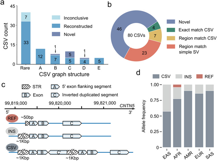
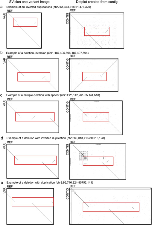
To explore novel CSV loci and structures, we further applied SVision to HG00733 data (~30X PacBio HiFi) released by HGSVC⁷, where CSVs were not well characterized. SVision detected 80 high-quality CSVs of 25 unique structures, 20 of which were novel, accounting for half of the events, and the rest five CSV graph structure matched frequently reported CSV types^{1, 2} (Extended Data Fig. 6, Supplementary Table S7, Supplementary File 4). We then introduced computational and experimental approaches to validate the structure and breakpoint junctions of those 80 CSV events. Firstly, GraphAligner¹⁶ was used to assess the internal structure and breakpoints of CSVs by aligning ONT reads¹⁷ of HG00733 to SVision CSV graphs (Online Methods). The graph alignments showed that single reads cover the entire paths of 79 CSV graphs, while one CSV graph path was covered by two different reads (Supplementary Table S8). Secondly, we found that 73 CSVs overlapped Phased Assembly Variant (PAV)⁷ calls, and 90% of them could be successfully reconstructed via haplotype contigs used by PAV for SV discovery (Fig. 2a), while others were challenging to characterize visually but could be verified via GraphAligner (Supplementary Table S8, Supplementary File 2). In addition, 20 CSVs were selected for inspection of assembly data and experimental validation after excluding SVs with breakpoints in annotated highly repetitive regions. Of these 20 CSVs, manual inspection confirmed that 18 events matched SVision’s reports, and two loci appeared to contain expansions of short tandem repeats that were collapsed in the reference (Supplementary Table S8). As for the experiment, eight CSVs failed PCR due to repetitive sequence or high GC content and the other 12 events were successfully confirmed by PCR and Sanger (Supplementary Table S8). The above validations indicate that SVision can detect and characterize CSV reliably from long-read data. Compared to 80 CSVs detected by SVision, short-read misinterpreted 23 as simple events and completely missed 46 CSVs (Supplementary Table S9), while 4 and 7 were fully and partially interpreted, respectively (Fig. 2b, Supplementary Table S9).

Fig. 2 ∣. Application of Svision on HG00733 HiFi data.

a, The Svision complex structural variants (CSVs) overlapping with Phased Assembly Variant (PAV) calls and reconstructed with phased HiFi contigs. The rare type represented multiple CSV graph structures, each of which contains fewer than five complex events. A: Inverted duplication. B: Deletion associated with inversion. C: Deletion associated with inverted duplication. D: Multiple deletion with spacer. E: Deletion associated with duplication. Inconclusive: Unable to characterize visually. Reconstructed: SVision CSV structure validated via contig based manual curation. Novel: No overlapping PAV call. b, Compared to 80 CSVs in HG00733 detected by SVision, short-read callset correctly reported the full structure of 4 CSVs (exact match), partially called 7 (region match), misinterpreted 23 events as simple (region match) and completely missed 46 CSVs. c, Three distinct alleles were found for the CNTN5 locus, including a contracted tandem repeat (REF), an expanded tandem repeat (INS), and an expanded tandem repeat with a complex duplication containing CNTN5 exon 4. d, The frequencies of three CNTN5 alleles differ among populations.

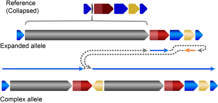
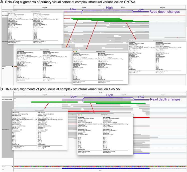
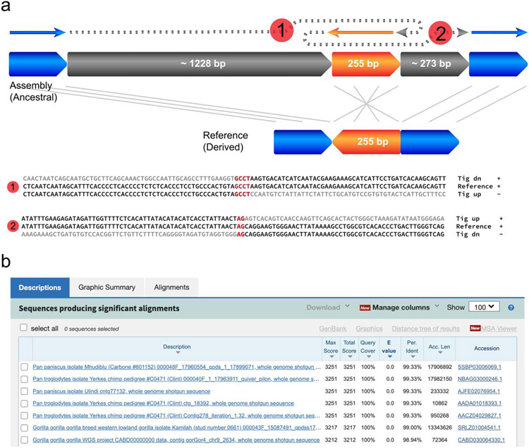
Of the 80 HG00733 CSVs detected by SVision, 19 (23.7%) overlapped 18 different genes (Supplementary Table S7). A complex duplication in CNTN5 (chr11:99,819,283-99,820,576), a neuronal gene expressed during development, is composed of a direct duplication of CNTN5 exon 4 and an inverted intronic duplication, both of which inserted in tandem within a CNTN5 intronic tandem repeat proximal to exon 4 (Fig. 2c, Extended Data Fig. 7). In a previous study⁷, this event was missed by short-reads, and PAV called only a simple insertion leaving the duplicated exon unannotated. Using the PAV calls and the SVision CSV structure, three distinct alleles were noted for this site, a contracted tandem repeat, an expanded tandem repeat, and an expanded tandem repeat containing the complex exon duplication (Fig. 2d, Supplementary Table S11, Supplementary File 3). We further observed the duplicated exon signature in the RNA-Seq data of human primary visual cortex and precuneus¹⁸ (Extended Data Fig. 8, Supplementary Table S11, Supplementary File 5). Additionally, SVision identified an insertion-inversion-insertion event (chr9:74,283,222-74,283,473), which was detected as a 1,737bp insertion by PAV but missed in previous long-read call sets^{17, 19}, except pbsv which called as a simple inversion (Extended Data Fig. 9a). This event was also re-genotyped by PanGenie²⁰, and it has 80% allele frequency among 2,504 unrelated samples in 1KGP cohort⁷. The inserted sequence of this CSV was also identified in chimpanzee and gorilla genomes (Extended Data Fig. 9b), indicating the insertion state was ancestral and the reference was derived via deletion and inversion.

In recent years, long-read sequencing technologies have revolutionized SV detection and revealed two times more variation than short reads^{7, 11}. While long-read SV detection tools have improved considerably in the past six years, none of them is able to correctly characterize multi-breakpoint events, leaving CSVs either uncalled or misinterpreted as simple SVs. Inspired by existing deep learning based variant detection methods^{21, 22}, SVision fills this gap by applying a multi-object recognition framework to denoised image to detect both simple and complex SVs, and autonomously identifies their structures without relying on predefined models. Taken together, SVision is a valuable tool to facilitate the study of complicated and novel CSVs, paving the way for the analysis of complex events at population-scale. Future adaptation to cancer genomes could further detection of novel complex structural variants in heterogenous cells.

Online Method

Evaluating simple structural variants detection with HG002.

To benchmark the performance of SV detection tools on HG002, we follow the procedure introduced by Genome-In-A-Bottle (GIAB) and adopted by CuteSV. Briefly, the high confidence insertion and deletion calls and high confidence regions published by the GIAB consortium are used as ground truth. The HiFi reads are aligned to reference hg19 by pbmm2 (https://github.com/PacificBiosciences/pbmm2, v1.4.0) with parameter ‘--preset CCS’, while ONT reads are aligned with pbmm2 default settings. The 5X and 10X coverage of HiFi and ONT data were further obtained with SAMtools²³ ‘-s’ option. Sniffles (v1.0.12), CuteSV (v1.0.10), pbsv (v2.2.2), SVision (v1.3.6) and SVIM (v1.4.0) were applied to the pbmm2 aligned file with default parameters. The minimum supporting read was 2 and 3 for 5X and 10X data, while 10 was used for the original coverage.

Simulating complex structural variants.

Ten complex structural variant (CSV) types were simulated according to frequently reported CSV types introduced by 1000 Genomes Project (1KGP)¹ and a cohort study of autism spectrum disorder (ASD)² (Supplementary Table S2, Supplementary Note). For the simulation, a CSV was essentially a combination of breakpoints from simple structural variants (SSVs). Therefore, a four-step simulation process was developed as follows. VISOR²⁴ was first used to simulate and to randomly implant five SSV types (deletion, inverted dispersed duplication, inverted tandem duplication, tandem duplication and dispersed duplication), on reference genome GRCh38. Secondly, we followed the procedure introduced by SURVIVOR²⁵ to simulate CSVs, where SSVs of the above five types were randomly added adjacent to the existing SSVs. In particular, 3,000 SSV of five types were created by VISOR with parameters ‘−n 3000 −r 20:20:20:20:20 −l 500 −s 150’. Then, we added extra variants required in predefined CSV structures to existing SSVs by following order of types, deletion, inverted dispersed duplication, inverted tandem duplication, tandem duplication and dispersed duplication. For instance, we first used deletions as seeds to create all deletion involved CSV instances, and turned to instances of next type. Finally, the variation genome with CSVs was used as input for the VISOR LASoR module to simulate 30X HiFi reads for subsequent alignment by ngmlr¹⁰ (v0.2.7) with the default setting. Note that VISOR is only used to simulate variants at one haplotype in this study (Supplementary Note).

Evaluating simulated complex structural variants detection.

To examine the correctness of detected CSVs, we used closeness and size similarity to assess whether two events are identical according to Truvari (https://github.com/spiralgenetics/truvari/) introduced by GIAB. The closeness bpDist and size similarity sim between prediction and benchmark were 500bp and 0.7, respectively. For example, assume a particular benchmark CSV [b.start, b.end, b.size], and a prediction [p.start, p.end, p.size]; then a correct region-match should satisfy the following equations:

$$\max (\mid \mathrm{b}.\text{start}-\mathrm{p}.\text{start}\mid ,\mid \mathrm{b}.\text{end}-\mathrm{p}.\text{end}\mid )\le \text{bp}\text{Dist}$$

$$\mathrm{b}.\text{size}\times \text{sim}\le \mathrm{p}.\text{size}\le \mathrm{b}.\text{size}\times (2-\text{sim})$$

Comparably, the exact-match not only required region-match but also required the correct detection of all subcomponent of CSV, including the subcomponent breakpoint type. Therefore, for a deletion-inversion that contained two subcomponents, e.g. inversion and deletion, the exact-match became a three-step evaluation:

1. Region-match between predicted CSV and benchmark deletion-inversion event.

2. For each subcomponent, we examine the breakpoint closeness and event size as well as the detected type.

3. The correct detection should pass condition 1) and 2). The subcomponent match is considered as either deletion or inversion correctly detected in 2).

In this study, we only considered INS, DEL, DUP and INV as subcomponent types in the evaluation. Any called CSVs without a matched prediction were counted as false negatives. Based on the numbers of true positives (TP) and false negatives (FN), we computed the recall, precision and F-score with the following equations, respectively.

$$\text{Precision}=\frac{\text{TP}}{\text{TP}+\text{FP}}$$

$$\text{Recall}=\frac{\text{TP}}{\text{TP}+\text{FN}}$$

$$\mathrm{F}-\text{score}=\frac{2\times \text{Precision}\times \text{Recall}}{\text{Precision}+\text{Recall}}$$

Each caller was run with different number of variant supporting read (i.e., 1, 3, 5 and 10), and the performance of detecting simulated CSVs was assessed correspondingly (Supplementary Table S3, Supplementary Note).

Examining complex structural variants detection in NA12878.

We used complex structural variants (CSV) from NA12878 to assess the performance of SVision. The CSV set of NA12878 was obtained from supplementary table 12 and 15 of a study conducted by the 1000 Genomes Project (1KGP)¹, containing 62 deletion and 251 inversion associated CSV sites in hg19 coordinates. We aligned the HiFi reads of NA12878 released by Human Genome Structural Variants Consortium (HGSVC)⁷ using ngmlr (v0.2.7) with the default setting for SVision SV detection. SAMtools was used to extract HiFi reads spanning the CSV loci, and Gepard²⁶ was used to create the Dotplots between HiFi reads and their corresponding reference sequences. We then manually inspected all Dotplots associated with a reported CVS locus (Supplementary File 1).

Three-channel coding of feature sequence.

SVision takes the sequence alignment file (BAM) and reference file as input. The encoder consisted of two major steps, i.e., variant feature sequence selection and sequence coding. Variant feature sequences are directly identified from long-read aberrant alignments containing SV signatures, such as inter-read and intra-read alignments. Intra-read alignments are derived from reads spanning the entire SV locus, while inter-read alignments are obtained from reads that are aligned to larger SV event, resulting in supplementary alignments. SVision identifies additional SV signatures by applying a k-mer based realignment approach for unmapped segment in feature sequence, such as ‘I’s from CIGAR string and gap sequence obtained from inter-read alignments. Then, sequence differences and similarities derived from matched and unmatched segments between variant feature sequence (VAR) and its corresponding segment on reference genome (referring to REF) is coded as an image (Supplementary Note). The image contains three channels, including (0, 0, 255), (0, 255, 0), and (255, 0, 0), to code the matched, the duplicated and the inverted segments, respectively. Given the three-channel image, SVision first creates the REF-to-REF image through k-mer realignment. As for VAR-to-REF image, matched segments obtained from CIGAR string and supplementary alignments, originating from aligner’s outputs, are directly used for image coding to reduce computational cost, and realignment results are further added to complete image coding. The denoised image is obtained by subtracting the REF-to-REF image from the VAR-to-REF image. Because the background is originated from reference sequence context, the encoder subtracts the segments of two images based on the REF sequence coordinates. Specifically, if segments from two images overlap on the reference dimension and their difference is larger than 50bp (minimum SV report size), the encoder keeps the non-overlapping part of the segment in the similarity image, where its coordinates are determined by VAR-to-REF image. Finally, the denoised image of each variant feature sequence is created and saved as matrix along with segment information tables for further process (Supplementary Note).

Detecting CSVs from denoised images via tMOR.

In principle, for each denoised image, the regions where VAR and REF are identical must be a straight line while SVs introduce discontinuous segments. These discontinuous segments indicating putative variants and their breakpoints in the denoised image are surrounded by segment signatures, which are considered as breakpoint object and further defined as Segment-of-Interest (SOI). Since long reads are likely to span more than one variant in the denoised image, the tMOR contains a two-step image segmentation process for further SOI recognition. Specifically, the tMOR first obtains a so-called one-variant image, from the denoised image based on the following steps (Supplementary Note).

1. Sorting and tagging. We sort all segments in the denoised image by their positions on read in ascending order. Then, the major segment is defined according to the matched segments derived from CIGAR operations, while the minor segment should meet one of the following conditions:

   Condition 1: the segment is derived from the hash-table based realignment.

   Condition 2: the segment is inverted compared to the reference genome.

   Condition 3: the segment is totally covered by another one.

2. Creating one-variant image. SVision partitions the denoised image into several one-variant images via sequential combination of the major segments. Specifically, each major segment and its neighboring major segment along with the minor segments (if they exist) between them are used to create a one-variant image.

Afterwards, SVision clusters similar one-variant images by measuring the distance of segment signatures between one-variant images. Thus, one-variant images in a cluster supports the same variant, and the size of a cluster is termed as the number of variant supporting image (Supplementary Note). Secondly, SVision collects SOIs from each one-variant image. Unlike traditional multi-object recognition that uses complex algorithms to select regions of interest, the segment signatures in the one-variant image enable efficient SOI identification by sequentially combining both major and minor segments. Then, SOIs are used as input for CNN prediction, and the interpreted SV types are given by the labels involved in the training set, including deletion (DEL), inversion (INV), insertion (INS), duplication (DUP) and tandem duplication (tDUP). The CNN assigns the probability score to assess the existence of variant subcomponents in the one-variant image (Supplementary Note).

Creating CSV graphs from one-variant images.

SVision uses a graph to unify the definition of different CSV types and provides a computational method to compare different CSV graph structures. To create a CSV graph G = (V, E), SVision first collects the node set V = V_s ∪ V_I ∪ V_D of G. Specifically, V_s = {S₁, S₂, … , S_n}, V_I = {I₁. I₂, … , I_m} and V_D = {D₁, D₂, … , D_k}, where n, m and k are the number of skeleton nodes, insertion nodes and duplication nodes in the graph, respectively. Skeleton nodes are derived from major segments in a one-variant image and sequence between discontinuous major segments on REF (i.e., concordant segments between VAR and REF). Insertion nodes consists of minor segments in one-variant image, while insertion nodes with known origins are defined as duplication nodes, representing duplicated segments in one-variant image. Moreover, each node v_i ∈ V is represented as a tuple V_i = (Seq, Pos, Strand), which represents a segment in the one-variant image. The Seq indicates the segment sequence, Pos is the position of the segment on VAR and Strand represents the forward or reverse strand of the segment. The edges in G is collected by E = E_ad ∪ E_dp. E_ad represents a set of adjacency edge ${\mathrm{e}}_{\text{ad}}^{\mathrm{k}}=({\mathrm{v}}_{\mathrm{k}},{\mathrm{v}}_{\mathrm{k}+1})$, connecting two adjacent nodes v_k and v_k+1, and E_dp represents a set of duplication edge e_dp, connecting the duplicated node with its known origin.

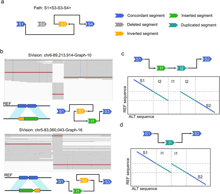
Given a graph G, a CSV could be interpreted by visiting each node through the E_ad edges. For example (Extended Data Fig. 10a), the CSV path is interpreted as “S1+S3-S3-S4+”, where ‘+’ or ‘-’indicates the direction of visiting a specific node, i.e., node Strand. Specifically, node S1 and S4 are visited in forward direction (+), while S3 is visited in reverse direction (−), so that the path should be “S1+S1+S3-S3-S4+S4+”. But for simplicity, only the intermediate nodes, such as S3, are kept twice, whereas the start node (S1) and the end node (S4) are used once in the path. The comparison of two graphs G₁ = (V₁, E₁) and G₂ = (V₂, E₂) is a NP-hard problem, but the ordered nodes based on the reference simplifies this problem. Therefore, SVision first compares the numbers of edges and nodes between two graphs G₁ and G₂, which are consider as different if either number is different. On the other hand, if graph G₁ and G₂ have topologically identical path in addition to the same numbers of nodes and edges, they are termed as isomorphic CSV graphs, i.e., G₁ = G₂. If graph G₁ and G₂ have the same numbers of nodes and edges but differ in paths, we further examine whether G₁ and G₂ share symmetric topology (Extended Data Fig. 10b), since a variant might be identified on either forward or minus strand, i.e., from 5’ to 3’ or from 3’ to 5’. In particular, we create a mirror graph G₁′ of the original graph G₁, and obtain a new path from G₁′. Similarly we also create G₂′ from G₂ Then, we cross compare whether the paths between G₁′ and G₂ as well as between G₂′ and G₁ are topologically identical. We consider G₁ and G₂ are isomorphic if both comparisons are equal. SVision keeps isomorphic graphs and symmetric graphs in two separate files, enabling search of CSV events of same structure. For each variant call, SVision keeps its all breakpoints in the “BKPS” column in the INFO field and a type (“SVTYPE” column). Especially for CSVs, their breakpoints are kept with both coordinates and associated graph structure in the “BKPS” and ‘GraphID’ column, respectively. Note that the ‘GraphID’ is used to search events of a specific graph structure in isomorphic and symmetric graph output files. Moreover, SVision involves the graph breakpoints induced from CSV Reference Graphical Fragment Assembly (rGFA) file in the ‘GraphBRPKS’ column. Note that the ‘GraphID’ and ‘GraphBRPKS’ columns are only reported when the parameter ‘--graph’ and ‘--qnames’ are activated.

Training data.

The CNN model in SVision is trained with both real and simulated simple SVs of DEL, INV, INS, DUP and tDUP, to avoid usually unbalanced numbers of SV types in real data. We obtained real SVs from NA19240 (4,282) and HG00514 (3,682) (Supplementary Note) by selecting calls supported by both PacBio CLR reads and Illumina reads¹⁷. In this integrated real SV set, we labeled SVs with the above-mentioned five rearrangement types. We further used VISOR to simulate SV events with the parameters ‘−n 4000 −r 20:20:20:20:20 −l 1000 −s 500’, and simulated the PacBio CLR reads. For all training SVs, their one-variant images and SOIs are created as we described in the above sections, leading to 75,000 SOIs (15,000 per type) in total, where 50% SOIs are from real events. These SOIs are shuffled for further CNN model training.

CNN model training.

SVision adopts AlexNet²⁷, a widely-used CNN model, to recognize sequence differences in similarity images. The AlexNet architecture consists of five convolutional layers and three fully-connected layers. Specifically, the first convolution layer loads images of size 224 × 224 × 3, and it uses the 11 × 11 × 3 convolution kernel with stride 4. The last three layers are fully connected and contains a five-class SoftMax layer with inputs from the five preceding convolution layers. In the end, the input SOIs are detected as either INS, DEL, INV, DUP, tDUP or mixed types for CSVs. We apply the idea of transfer learning to train CNN with 75,000 SOIs. First, the parameters of all layers in the CNN are initialized to the best parameter set that was achieved on the ImageNet competition. Afterwards, we fine-tune the parameters of the last three fully-connected layers on our data using back propagation and gradient descent optimization with a learning rate of 0.001. The loss function is defined as the cross entropy between predicted probability and the true class labels. Moreover, SVision’s CNN architecture is lightweight and has far fewer layers than complex CNN models such as ResNet and Inception V3, which results in a highly efficient fine-tuning process with large batch size (default: 128) even on a CPU machine. To evaluate the trained CNN model, we apply ten-fold cross validation and examine the loss and accuracy of each model on the training set. To further assess the accuracy of a model, the trained model at each round is applied to an independent test set of 7,500 SOIs derived from simulated SVs. Finally, SVision selects the model with the best performance (Supplementary Note).

Quality score of discoveries.

SVision uses a score function to measure the quality of each discovery based on consistency and prediction reliability derived from one-variant image clusters.

1. One-variant image consistency. Intuitively, the non-linear segments in a given one-variant image indicate potential differences between REF and VAR. We thus first compute the non-linear score for all images that support each event, i.e., one-variant images originated from a variant feature sequence cluster. The non-linear score of a one-variant image is calculated by its segments coordinates and lengths. Specifically, for a one-variant image with segments:

   $${\text{Nonlinear score}}_{\mathrm{i}}=\frac{{\sum }_k(\mid \mathrm{k}.{\text{ref}}_{\text{mid}}-\mathrm{k}.{\text{read}}_{\text{mid}}\mid )\times \mathrm{k}.\text{length}}{\text{RefSpan}}$$

   where the summation is over all segments k in image ref_mid and k. read_mid are the center of segment on reference and read, respectively. Then we normalize the summation by dividing RefSpan, which denotes the distance between the leftmost and rightmost coordinates of the similarity image. Finally, for a SV of M supporting images, we calculate the consistency score with the following equation:

   $$\text{Consistency}=\frac{\text{Std}(\{{\text{nonlinear score}}_1,\dots ,{\text{nonlinear score}}_{\mathrm{M}}\})}{\mathrm{M}}$$

   Accordingly, we expect a smaller consistency value for high-quality SV predictions.
2. Prediction reliability. This part evaluates the deep learning prediction quality. The last layer in the CNN architecture is a SoftMax layer, which outputs the probability of the prediction results. Therefore, we use the average probability of all SOIs as the CNN reliability:

   $$\text{Reliability}=\frac{{\sum }_s\mathrm{s}.\text{softmax}\times 100}{\#\text{SOIs}}$$

   where the summation is over all SOIs in an one-variant image. The reliability will range from 0 to 100 because the SoftMax probabilities always range from 0 to 1. We expect higher reliability values for accurate SVs.

Finally, we summed up the two features and normalized it to range from 0 to 100:

$$\text{qual}=\text{Consistency}+(1-\text{Reliability})$$

$$\text{Normalized score}=(1-\frac{\text{sum}(\text{Scores})-\text{min}(\text{Scores})}{\max (\text{Scores})-\text{min}(\text{Scores})})\times 100$$

where Scores = {qual₁,…, qual_M}, M is the total number of images supporting this variant.

Analysis of CSVs detected from HG00733.

SVision was run under the default setting except parameters ‘-s 5 --graph --qname’. The HiFi reads of HG00733 were aligned to reference GRCh38 by ngmlr (v0.2.7) with the default setting. Firstly, the events detected by SVsion at low mapping quality regions, centromeres, genome gap regions, and etc. were excluded in analysis. These regions were obtained from https://github.com/mills-lab/svelter/tree/master/Support/GRCh38 and the UCSC genome centromere for reference GRCh38. Then, we applied the following steps to filter CSVs from the raw callset. 1) Filtering CSVs of length larger than 100kbp; 2) Filtering CSVs without complete graph representation, where the path ends with other node types instead of ‘S’ and 3) For multiple CSVs at one site, we only kept the one with the most number of supporting reads. SVision revealed two special complex structures, i.e., a structure consists of nodes ‘S:2,I:2,D:1’ and path ‘S1+I1+I1+I2+I2+S2+’ as well as another structure consists of nodes ‘S:2,I:1,D:1’ and path ‘S1+I1+I1+S2+’, which were visually confirmed as local targeted site duplication (Extended Data Fig. 10c) and tandem duplication (Extended Data Fig. 10d). Events of these two structures were also filtered because they were considered as simple events from biological perspective. Afterwards, we used RepeatMasker and tandem repeat finder (TRF) annotated files from UCSC genome browser to annotate the CSVs passed the filters through BEDtools²⁸ intersect option. The repeat type was assigned if the CSV region overlaps with the repeat element, while the size or percentage of overlaps was not required. For CSVs with multiple repeat types, the one with the largest overlapping region with the CSV was chosen. Meanwhile, CSV was annotated as STR if the repeat unit length < 7bp, otherwise, it was annotated as VNTR. Finally, we termed all CSVs that outside of VNTR/STR regions as high-quality CSVs, which were further validated and used for further analysis. The PAV and short-read data matched CSV loci were obtained through BEDtools without requiring overlap size. For the short-read data, a matched CSV locus was considered as completely reconstructed if both breakpoint positions and types matched what SVision reported, otherwise as partially reconstructed events if either breakpoints or types agreed with SVision’s prediction.

The PAV merged call set from 35 haplotype-resolved samples was used to explore the frequency of CSV on CNTN5 (Supplementary Table S11). In addition, the RNA-Seq data of precuneus and primary visual cortex from both control and disease samples were obtained from a recent study of Alzheimer’s disease¹⁸ to understand the potential functional impact of CSV on CNTN5 (Supplementary Table S12). The paired-end RNA data was aligned with hisat2 default setting, from which the duplicated exon signature could be observed from discordant read-pair alignment, i.e., read-pair aligned in reverse and forward direction (Extended Data Fig. 8). For the insertion-inversion-insertion event at chr9:74,283,222-74,283,473 detected by SVision, it was reported as insertion of variant id chr9-74283228-INS-1797 by a recent study conducted by HGSVC⁷ (Supplementary Note). The insertional sequence was extracted from HiFi assembly and Blast against several primate genomes. Moreover, the assembly of chimpanzee and gorilla were mapped to GRCh38 with minimap2 and called variant with PAV, from which the same insertion event was identified.

Validation of high-quality CSVs detected from HG00733.

We validated 80 CSVs detected by SVision in HG00733 via 1) graph-based alignment; 2) contig-based visual confirmation and 3) PCR and Sanger sequencing.

Graph-based alignment.

For each CSV graph in rGFA format, we extracted the CSV locus spanning reads with SAMtools and aligned these reads to each CSV graph via GraphAligner (v1.0.12) with the default setting. A CSV was successfully validated if a single ONT read could be aligned to the corresponding variant path specified in the rGFA file. We then counted the number of long reads covering the entire VAR path as the number of support for this CSV event.

Contig-based visual confirmation.

To examine the internal structure of CSVs, the phased-assembly specified in the PAV (v1.1.2, TIG_REGION column) at the reported variant region was used for further analysis. We first extracted the contig sequence harboring variant based on the coordinates provided in the ‘PAV_TIG_REGION’ (Supplementary Table S8). For example, a sequence containing variant was extracted from the h1 assembled genome for ‘1∣1’ and ‘1∣0’ genotype, while from h2 assembled genome for ‘0∣1’. In order to validate CSV structure containing complex insertion, we extended 5Kbp both upstream and downstream the CSV region to extract the reference genome via BEDtools getfasta option, from which the origin of the inserted sequence could be identified. Afterwards, Gepard was used to create the Dotplot of contig sequence (y-axis in the Dotplot) and reference sequence (x-axis in the Dotplot) for each CSV locus. Based on each contig Dotplot, the manual validation contained two tiers of metrics: 1) whether the reported region contains a variant; and 2) whether the SVision reported structure is identical to what revealed by Dotplot. A CSV was considered completely reconstructed if both 1) and 2) were satisfied, while others were considered as inconclusive events.

PCR and Sanger sequencing.

We first determined that about half of the 80 CSVs (39/80) were intractable for PCR due to their location within segmental duplications, the size of the amplicon needed to validate the rearrangement, or the simple repeat nature of the rearrangement. We then randomly selected 20 of the remaining rearrangements, and performed BLAT on the local region from the HG0733 assembly data. We next attempted to PCR each of the 20 CSVs. Briefly, we designed primers flanking the CSV or flanking breakpoints within the CSV for each of the 20 events (Supplemental Table S14). Next, we attempted to amplify each region using Takara LA taq. We obtained the predicted band size for 12 of the 20 variant loci; the remaining 8 regions did not amplify in 3 separate attempts with alterations of the PCR conditions and template amounts. All PCR products were sent to Sanger sequencing and validated as on target, and contained the correct amplicon with the breakpoint from the assembly and SVision call.

Extended Data

Extended Data Fig. 1 ∣. Diagram of example simple and complex structural variants and their aberrant alignment patterns.

a, The diagram and alignment pattern of a simple deletion. b, The diagram and alignment pattern of a deletion associated with inversion, where the inverted segment occurred at the 3’ flank region of the deletion.

Extended Data Fig. 2 ∣. Performance evaluation of callers with HG002 truthset at different coverages and platforms.

a, F-score of callers on different platforms evaluated with Truvari. b, The precision (x-axis), recall (y-axis) and F-score (F, dotted line) measurements of detecting SVs from HiFi data at different coverages. c, The precision and recall measurements of detecting SVs from ONT data at different coverages. It should be noted that this evaluation ignored SV genotype, but only evaluated on event level.

Extended Data Fig. 3 ∣. Simulated complex structural variant types and performance of detecting complex structural variant subcomponents.

a, The diagrams of simulated complex structural variants (CSV). Each type has a unique ID and a type definition. b, The size distribution of simulated CSVs smaller than 1Kbp (1,200 events). c, The size distribution of simulated CSVs larger than 1Kbp (1,800 events). d, The region-match recall rates of model-based callers for detecting subcomponents (i.e., DUP-duplication, DEL-deletion, INV-inversion) of CSVs.

Extended Data Fig. 4 ∣. The diagrams and alignment patterns of two unclassified complex structural variants.

a, SVision correctly detected a deleted sequence replaced with dispersed duplication and inverted duplication. b, SVision characterized a complex insertion, consisting of two dispersed duplications and one inverted duplication. Both types of (a) and (b) are labeled as unclassified (NA) in the 1KGP call set. The top panel of (a) and (b) are the discordant alignments derived from short-read sequencing (i.e., one end unmapped and discordant alignment). The bottom panels of (a) and (b) describe the abnormal alignments from long-read alignment.

Extended Data Fig. 5 ∣. One example of simple deletion misinterpreted as complex event by short-read data due to local repeats.

a, Two Dotplots are created with Gepard to illustrate the local repeats at the variant locus on the reference genome (left) and the breakpoints comparing HiFi read (READ, y-axis) and the reference genome (REF, x-axis). b, The IGV view at this locus with reads grouped by pair orientation and colored by insert-size and pair orientation.

Extended Data Fig. 6 ∣. Examples of reported complex structural variant types identified by SVision.

a, One of the 12 inverted duplication events detected by SVision and classified as CSV graph structure ‘12’, b, One of the eight deletion associated with inversion events detected by SVison and classified as CSV graph structure ‘15’. c, One of the five multiple-deletion with spacer events detected by SVision and classified as CSV graph structure ‘27’. d, One of ten deletion with inverted duplication events detected by SVision and classified as CSV graph structure ‘23’. e, One of the five deletion with duplication events detected by SVision and classified as CSV graph structure ‘28’. From figure (a) to (e), the Dotplots on the left column are SVision one-variant images created with variant feature sequence (VAR, y-axis) and reference sequence (REF, x-axis) at the variant loci, while the Dotplots on right column are created with variant spanning HiFi assemblies (CONTIG, y-axis) and the reference sequence (REF, x-axis) at the variant loci.

Extended Data Fig. 7 ∣. The HiFi assembly reconstruction of the expanded allele and complex structural variant allele affecting CNTN5.

The grey region indicates the repeat expansion. The dark red region indicates exon 4 of CNTN5, while the light red region is the 5’ flanking region of the exon.

Extended Data Fig. 8 ∣. The IGV screenshot of duplicated CNTN5 exon signature observed in RNA-Seq data.

a, The RNA-Seq data of the primary visual cortex from an Alzheimer disease female. b, The RNA-Seq data of a control male precuneus. In (a) and (b), the green bars pointed by red arrows are duplication like read-pair signatures, i.e., there are 4 supporting discordant read-pairs in (a), and 2 in (b). Moreover, read depth change (fitted by purple line) on exon is observed in both (a) and (b). The RNA-Seq data for (a) and (b) are obtained from Sequence Read Archive (SRA) with accession number SRR14194220 and SRR14194206, respectively.

Extended Data Fig. 9 ∣. The ancestral state of one genome segment revealed by a complex structural variant.

a, The structure and breakpoint junction sequence of the variant derived from HiFi assembly. b, Blastn results of the inserted sequence mapping to primate genomes, and the top hits include pan troglodytes and gorilla.

Extended Data Fig. 10 ∣. Examples of graph and symmetric graphs as well as two special complex events identified by SVision.

a, An example of a complex structural variant (CSV) graph where its graph path is interpreted as S1+S3-S3-S4+. b, Examples of isomorphic graphs representing two different CSV events. c, SVision detected CSV classified as local target site duplication. d, SVision detected CSV classified as tandem duplication. Though events of structure depicted by (c) and (d) were computed as complex events, they were considered as simple events from the biological perspective.

Code availability

The SVision program (v1.3.6) and trained model are provided at GitHub (https://github.com/xjtu-omics/SVision).

Data availability

Both the HiFi and Oxford Nanopore sequencing data for HG002 are available at GIAB FTP site (ftp://ftp.ncbi.nlm.nih.gov/giab/ftp/data/AshkenazimTrio/HG002_NA24385_son/). The PacBio HiFi sequencing data. For NA12878 is available at http://ftp.1000genomes.ebi.ac.uk/vol1/ftp/data_collections/HGSVC2/release/v1.0/assemblies/20200628_HHU_assembly-results_CCS_v12/haploid_reads/. Primary raw PacBio HiFi sequencing data for HG00733 is from http://ftp.1000genomes.ebi.ac.uk/vol1/ftp/data_collections/HGSVC2/working/20190925_PUR_PacBio_HiFi/, and the high-quality phased assemblies is available at http://ftp.1000genomes.ebi.ac.uk/vol1/ftp/data_collections/HGSVC2/working/20200417_Marschall-Eichler_NBT_hap-assm/. The Oxford Nanopore sequencing data used for graph-based validation is from http://ftp.1000genomes.ebi.ac.uk/vol1/ftp/data_collections/hgsv_sv_discovery/working/20181210_ONT_rebasecalled/. The latest HG00733 PAV (v1.1.2) call is from http://ftp.1000genomes.ebi.ac.uk/vol1/ftp/data_collections/HGSVC2/working/20210806_PAV_VCF/, and the latest release of PAV calls for 35 samples is from http://ftp.1000genomes.ebi.ac.uk/vol1/ftp/data_collections/HGSVC2/release/v2.0/integrated_callset/. The RNA-Seq data of precuneus and primary visual cortex could be accessed in SRA with PRJNA720779. All results generated by this study are available in Supplementary Note from the article.

References

- 1.Sudmant PH et al. An integrated map of structural variation in 2,504 human genomes. Nature 526, 75–81 (2015). [DOI] [PMC free article] [PubMed] [Google Scholar]
- 2.Collins RL et al. Defining the diverse spectrum of inversions, complex structural variation, and chromothripsis in the morbid human genome. Genome Biol 18, 36 (2017). [DOI] [PMC free article] [PubMed] [Google Scholar]
- 3.Li Y et al. Patterns of somatic structural variation in human cancer genomes. Nature 578, 112–121 (2020). [DOI] [PMC free article] [PubMed] [Google Scholar]
- 4.Fujimoto A et al. Whole-genome sequencing with long reads reveals complex structure and origin of structural variation in human genetic variations and somatic mutations in cancer. Genome Med 13, 65 (2021). [DOI] [PMC free article] [PubMed] [Google Scholar]
- 5.Baca SC et al. Punctuated evolution of prostate cancer genomes. Cell 153, 666–677 (2013). [DOI] [PMC free article] [PubMed] [Google Scholar]
- 6.Quinlan AR & Hall IM Characterizing complex structural variation in germline and somatic genomes. Trends Genet 28, 43–53 (2012). [DOI] [PMC free article] [PubMed] [Google Scholar]
- 7.Ebert P et al. Haplotype-resolved diverse human genomes and integrated analysis of structural variation. Science 372 (2021). [DOI] [PMC free article] [PubMed] [Google Scholar]
- 8.Aganezov S et al. Comprehensive analysis of structural variants in breast cancer genomes using single-molecule sequencing. Genome Res 30, 1258–1273 (2020). [DOI] [PMC free article] [PubMed] [Google Scholar]
- 9.Alkan C, Coe BP & Eichler EE Genome structural variation discovery and genotyping. Nat Rev Genet 12, 363–376 (2011). [DOI] [PMC free article] [PubMed] [Google Scholar]
- 10.Sedlazeck FJ et al. Accurate detection of complex structural variations using single-molecule sequencing. Nat Methods 15, 461–468 (2018). [DOI] [PMC free article] [PubMed] [Google Scholar]
- 11.Ho SS, Urban AE & Mills RE Structural variation in the sequencing era. Nat Rev Genet 21, 171–189 (2020). [DOI] [PMC free article] [PubMed] [Google Scholar]
- 12.Li H, Feng X & Chu C The design and construction of reference pangenome graphs with minigraph. Genome Biol 21, 265 (2020). [DOI] [PMC free article] [PubMed] [Google Scholar]
- 13.Jiang T et al. Long-read-based human genomic structural variation detection with cuteSV. Genome Biol 21, 189 (2020). [DOI] [PMC free article] [PubMed] [Google Scholar]
- 14.Heller D & Vingron M SVIM: structural variant identification using mapped long reads. Bioinformatics 35, 2907–2915 (2019). [DOI] [PMC free article] [PubMed] [Google Scholar]
- 15.Zook JM et al. A robust benchmark for detection of germline large deletions and insertions. Nat Biotechnol 38, 1347–1355 (2020). [DOI] [PMC free article] [PubMed] [Google Scholar]
- 16.Rautiainen M & Marschall T GraphAligner: rapid and versatile sequence-to-graph alignment. Genome Biol 21, 253 (2020). [DOI] [PMC free article] [PubMed] [Google Scholar]
- 17.Chaisson MJP et al. Multi-platform discovery of haplotype-resolved structural variation in human genomes. Nat Commun 10, 1784 (2019). [DOI] [PMC free article] [PubMed] [Google Scholar]
- 18.Guennewig B et al. Defining early changes in Alzheimer's disease from RNA sequencing of brain regions differentially affected by pathology. Sci Rep 11, 4865 (2021). [DOI] [PMC free article] [PubMed] [Google Scholar]
- 19.Audano PA et al. Characterizing the Major Structural Variant Alleles of the Human Genome. Cell 176, 663–675 e619 (2019). [DOI] [PMC free article] [PubMed] [Google Scholar]
- 20.Ebler J et al. Pangenome-based genome inference. bioRxiv (2020). [Google Scholar]
- 21.Poplin R et al. A universal SNP and small-indel variant caller using deep neural networks. Nat Biotechnol 36, 983–987 (2018). [DOI] [PubMed] [Google Scholar]
- 22.Cai L, Wu Y & Gao J DeepSV: accurate calling of genomic deletions from high-throughput sequencing data using deep convolutional neural network. BMC Bioinformatics 20, 665 (2019). [DOI] [PMC free article] [PubMed] [Google Scholar]
- 23.Li H et al. The Sequence Alignment/Map format and SAMtools. Bioinformatics 25, 2078–2079 (2009). [DOI] [PMC free article] [PubMed] [Google Scholar]
- 24.Bolognini D et al. VISOR: a versatile haplotype-aware structural variant simulator for short- and long-read sequencing. Bioinformatics 36, 1267–1269 (2020). [DOI] [PubMed] [Google Scholar]
- 25.Jeffares DC et al. Transient structural variations have strong effects on quantitative traits and reproductive isolation in fission yeast. Nat Commun 8, 14061 (2017). [DOI] [PMC free article] [PubMed] [Google Scholar]
- 26.Krumsiek J, Arnold R & Rattei T Gepard: a rapid and sensitive tool for creating dotplots on genome scale. Bioinformatics 23, 1026–1028 (2007). [DOI] [PubMed] [Google Scholar]
- 27.Krizhevsky A, Sutskever I & Hinton GE in Proceedings of the 25th International Conference on Neural Information Processing Systems - Volume 1 1097–1105 (Curran Associates Inc., Lake Tahoe, Nevada; 2012). [Google Scholar]
- 28.Quinlan AR & Hall IM BEDTools: a flexible suite of utilities for comparing genomic features. Bioinformatics 26, 841–842 (2010). [DOI] [PMC free article] [PubMed] [Google Scholar]
Associated Data
This section collects any data citations, data availability statements, or supplementary materials included in this article.
Supplementary Materials
Data Availability Statement