Quantitative Imaging Biomarkers: A Review of Statistical Methods for Computer Algorithm Comparisons

Abstract

Quantitative biomarkers from medical images are becoming important tools for clinical diagnosis, staging, monitoring, treatment planning, and development of new therapies. While there is a rich history of the development of quantitative imaging biomarker (QIB) techniques, little attention has been paid to the validation and comparison of the computer algorithms that implement the QIB measurements. In this paper we provide a framework for QIB algorithm comparisons. We first review and compare various study designs, including designs with the true value (e.g. phantoms, digital reference images, and zero-change studies), designs with a reference standard (e.g. studies testing equivalence with a reference standard), and designs without a reference standard (e.g. agreement studies and studies of algorithm precision). The statistical methods for comparing QIB algorithms are then presented for various study types using both aggregate and disaggregate approaches. We propose a series of steps for establishing the performance of a QIB algorithm, identify limitations in the current statistical literature, and suggest future directions for research.

1. Background and Problem Statement

Medical imaging is an effective tool for clinical diagnosis, staging, monitoring, treatment planning, and assessing response to therapy. In addition it is a powerful tool in the development of new therapies. Measurements of anatomical, physiological, and biochemical characteristics of the body through medical imaging, referred to as quantitative imaging biomarkers (QIBs), are becoming increasingly used in clinical research for drug and medical device development and clinical decision-making.

A biomarker is defined generically as an objectively measured indicator of a normal or pathological process or pharmacologic response to treatment [1,2]. In this paper, we focus on QIBs, defined as imaging biomarkers which consist of a measurand only (variable of interest) or measurand and other factors (e.g. body weight) that may be held constant and the difference between two values of the QIB is meaningful. In many cases there is a clear definition of zero such that the ratio of two values of the QIB is meaningful [3,4].

Most QIBs requires a computation algorithm, which may be simple or highly complex. An example of a simple computation is measurement of a nodule diameter on a 2D x-ray image. A slightly more complex example is the estimation of the value of the voxel with the highest standardized uptake value (SUV, a measure of relative tracer uptake) within a pre-defined region of interest in a volumetric positron emission tomography (PET) image. Even more complex methods exist, such as the estimation of K^trans, the volume transfer constant between the vascular space and the extravascular, extracellular space from a dynamic contrast-agent-enhanced magnetic resonance imaging (MRI) sequence, where an a priori physiological model is used to fit the measured time-dependent contrast enhancement measurements. In this paper we consider QIBs generated from computer algorithms, whether or not the computer algorithm requires human involvement.

While there is a rich history of the development of QIB techniques, there has been comparatively little attention paid to the evaluation and comparison of the algorithms used to produce the QIB results. Estimation errors in algorithm output can arise from several sources during both image formation and the algorithmic estimation of the QIB (see Figure 1). These errors combine (additively or non-additively) with the inherent underlying biological variation of the biomarker. Studies are thus needed to evaluate the imaging biomarker assay with respect to bias, defined as the expected difference between the biomarker measurement (measurand) and the true value [3], and precision, defined as the closeness of agreement between values of the biomarker measurement on the same experimental unit [3].

Figure 1.

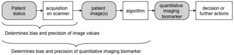
The role of quantitative medical imaging algorithms and dependency of the estimated QIB on sources of bias and precision.

There are several challenges in the evaluation and adoption of QIB algorithms. A recurring issue is the lack of reported estimation errors associated with the output of the QIB. One example is the routine reporting in clinical reports of PET SUVs with no confidence intervals to quantify measurement uncertainty. If the measure of a patient's disease progression versus response to therapy is determined based on changes of SUV ± 30%, for example, then the need to state the SUV measurement uncertainties for each scan becomes apparent.

Another challenge is the inappropriate choice of biomarker metrics and/or parametric statistics. For example, tumor volume doubling time is sometimes used in studies as a QIB. However it may not be appropriate to use the mean as the parametric statistic for an inverted, non-normal, measurement space. Since a zero growth rate corresponds to a doubling time of infinity, it is easy to see that parametric statistics based on tumor volume doubling time (e.g., mean doubling time) may be skewed and/or not properly representative of the population. See Yankelevitz [5] and Lindell et al [6] for further discussion.

Confidence intervals, or some variant thereof, are needed for a valid metrology standard. However, many studies inappropriately use tests of significance, e.g., p-values, in place of appropriate metrics. In addition, there may be discordance between what might be a superior metric statistically and what is clinically acceptable or considered clinically relevant. For example, a more precise measuring method will typically better predict the medical condition, but only until the measurement precision exceeds normal biological variation; further improvement in precision will offer no significant improvement in efficacy. Finally, when potentially improved algorithms are developed, data from previous studies are often not in a form that allows new algorithms to be tested against the original data. Publicly available databases of clinical images are being developed to provide a resource of images with appropriate documentation that may be used for computer algorithm evaluation and comparison. Three notable examples are 1) the Lung Imaging Database Consortium (LIDC), which makes available a database of computed tomography (CT) images of lung lesions that have been evaluated by experienced radiologists for comparison of lesion detection and segmentation algorithms [7], 2) the Reference Image Database for Evaluation of Response (RIDER), which contains sets of CT, PET and PET/CT patient images before and after therapy, as well as test/retest, assumed zero-change, MR data sets from phantoms, human brain and breast [8] (https://wiki.nci.nih.gov/display/CIP/RIDER), and 3) the Retrospective Image Registration Evaluation Project (www.insight-journal.org/rire/), which allows open source data retrospective comparisons of CT-MRI and PET-MRI image registration techniques. Other such databases can be found at http://www.via.cornell.edu/databases/.

This paper is motivated by the activities of the Radiological Society of North America (RSNA) Quantitative Imaging Biomarkers Alliance (QIBA) [9]. The mission of QIBA is to improve the value and practicality of quantitative imaging biomarkers by reducing variability across devices, patients, and time. A cornerstone of the QIBA methodology is to produce a description of a QIB in sufficient detail that it can be considered a validated assay [4], which means that the measurement bias and variability are both characterized and minimized. This is accomplished through the use of a QIBA ‘Profile’, which is a document intended for a broad audience including scanner and third-party device manufacturers (e.g., display stations), pharmaceutical companies, diagnostic agent manufacturers, medical imaging sites, imaging contract research organizations, physicians, technologists, researchers, professional organizations, and accreditation and regulatory authorities. A QIBA Profile has the following components:

1. A description of the intended use of, or clinical context for, the QIB.

2. A ‘claim’ of the achievable minimum variability and/or bias.

3. A description of the image acquisition protocol needed to meet the QIBA claim.

4. A description of compliance items needed to meet the QIBA claim.

In a QIBA Profile, the claim is the central result, and describes the QIB as a standardized, reproducible assay in terms of technical performance. The QIBA claim is based on peer-reviewed results as much as possible, and also represents a consensus opinion by recognized experts in the imaging modality. For example, the QIBA fluorodeoxyglucose (FDG)-PET/CT Profile [10] was based on nine original research studies [11-19], one meta-analysis [20], and two multi-center studies that are in the process of being submitted for publication, as well as review by over 100 experts. During the initial development of the Profiles from the various QIBA Technical Committees, it was realized that different metrics were being used to describe the minimum achievable variability and/or bias, and that quantitative comparisons of the corresponding QIBs required a careful description of the goals of the comparison, the available data, and the means of comparison. This comparison is an important precursor to the final goal (Figure 1) of providing information as a tool for clinical imaging or in clinical trials.

The specific goals of this paper are to provide a framework for QIB algorithm comparisons by a review and critique of study design (Section 2), general statistical hypothesis testing and confidence interval methods as they commonly apply to QIBs (Section 3), followed by several sections on statistical methods for algorithm comparison. First we address approaches to estimating and comparing algorithms' bias when the true value or a reference standard is present (Section 4); then we address the more difficult task of estimating and comparing bias when there is no true value or suitable reference standard available (Section 5). In Section 6 we review the statistical methods for assessing agreement and reliability among QIB algorithms. We discuss methods for estimating and comparing algorithms' precision in Section 7. Finally, we link the preceding sections to a process for establishing the effectiveness of QIBs for implementation or marketing with defined technical performance claims (Section 8). There is a discussion of future directions in Section 9.

2. Study Design Issues for QIB Algorithm Comparisons

There are two common types of studies for comparing QIB algorithms: (a) studies to characterize the bias and precision in the measuring device/imaging algorithm/assay, and (b) studies to determine the clinical efficacy of the biomarker. It is the former that is the main focus of this paper. Clinical efficacy requires a distinct set of study questions, designs, and statistical approaches to address and is beyond the scope of this paper. Once a QIB has been optimized to minimize measurement bias and precision, then traditional clinical studies to evaluate clinical efficacy may be conducted. Efficacy for clinical practice can be evaluated from clinical studies that correlate clinical outcomes to one or more measurements for the biomarker.

There are several different QIB types (Table 1). When designing a study it is important to evaluate and report the correct measurement type. For example, in measuring lesion size there are at least three different measurement types: absolute size assessed from a single image, a change in size assessed from a sequential pair of images, and growth rate assessed from two or more images recorded at known time intervals. Each of these has a different measurand and associated uncertainty; characterizing one type does not mean that other types are characterized. A related issue is the suitability of a measurand for statistical analysis. For example, if in a set of change-in-size measurements one case has a measured value of no change (i.e. zero) then the doubling time for that case is infinity. Further estimating the mean doubling time for a set of cases that include this case will also have a value of infinity. If the reciprocal scale of growth rate is used for a study then these problems do not occur. The results of the study can be translated back to the doubling times for presentation in the discussion.

Table 1. Types of QIB Measurements with Example.

Measurement Type	Parameters	Measurand	Examples and Explanations
Extent	Single Image	V, L, A, D, I, SUV	Volume (V), Length (L), Area (A), Diameter in 2D image (D), Intensity (I) of an image or region of interest (ROI), SUV (a measure of relative tracer uptake).
Geometric form	Single or multiple images	VX, AX	Set of locations of all the pixels or voxels that comprise an object in an image or ROI; the overlap of two images.
Geometric location	Single or multiple images	Distance	Distance relative to the true value or reference standard or between two measurements; distance between two centers of mass; location of a peak.
Proportional Change	Two or more repeat images	$\frac{2({\mathrm{V}}_2-{\mathrm{V}}_1)}{({\mathrm{V}}_1+{\mathrm{V}}_2)}$	Fractional change in A or V or L or D or I measured from ROIs of two or more images. Response-to-therapy may be indicated by a lesion increasing in size (progression of disease = PD), not changing in size (stable disease = SD), or decreasing in size (response to therapy = RT). The magnitude of the change may also be important (e.g. cardiac ejection fraction).
Growth Rate	Two or more repeat images and time intervals	[(V2 / V1)1/Δt − 1]	Proportional change per unit time in A or V or D or I of an ROI from two or more images with respect to an interval of time Δt. Malignant lesions are considered to have a high approximately constant growth rate (i.e., have volumes that increase exponentially in time). Benign nodules are usually slow growing.
Morphological and Texture Features	Single or multiple images	CIR, IR, MS, AF, SGLDM, FD, FT, EM	Boundary Aspects including surface curvature such as Circularity (CIR), Irregularity (IR), and Boundary Gradients such as Margin Sharpness (MS). Texture Features of an ROI: Grey level statistics, Autocorrelation function (AF), Spatial Gray Level Dependence Measures (SGLDM), Fractal dimension measures (FD), Fourier Transform measures (FT), Energy Measures (EM).
Kinetic response	Two or more repeat images during the same session	f(t), Ktrans, ROI(t)	The values of pixels change due to the response to an external stimulus, such as the uptake of an intravenous contrast agent (e.g., yielding Ktrans) or an uptake of a radioisotope tracer (ROI(t)). The change in these values is related to a kinetic model.
Multiple acquisition protocols	Two or more repeat images with different protocols during same session	ADC, BMD, fractional anisotropy	ADC=apparent diffusion coefficient, BMD=bone mineral density. Unlike other QIBs considered here, morphological and texture features may not be evaluable with some of the statistical methods described since they do not usually have a well-defined objective function.

There is a number of common research questions asked in QIB algorithm comparison studies. They range from which algorithms have lower bias and more precision to more complex questions such as which algorithms are equivalent to a reference standard. Different study designs are needed to answer these questions. Table 2 lists several common questions addressed in QIB comparison studies and the corresponding design requirements needed.

Table 2. Common Research Questions and Corresponding Design Requirements.

Research Question:	Study Design Requirements
1. Which algorithm(s) provides measurements such that the mean of the measurements for an individual subject is closest to the true value for that subject (comparison of individual bias)?	The true value, and replicate measurements by each algorithm for each subject
2. Which algorithm(s) provides the most precise measurements under identical testing conditions (comparison of repeatability)?	Replicate measurements by each algorithm for each subject
3. Which algorithm(s) provides the most precise measurements under testing conditions that vary in location, operator, or measurement system* (comparison of reproducibility)?	One or more replicate measurements for each testing condition by each algorithm for each subject
4. Which algorithm provides the closest measurement to the truth (comparison of aggregate performance)?	The true value, and one or more replicate measurements by each algorithm for each subject
5. Which algorithm(s) are interchangeable with a Reference Standard (assessment of individual agreement)?	Replicate measurements by the reference standard for each subject, and one or more replicate measurements by each algorithm for each subject
6. Which algorithm(s) agree with each other (assessment of agreement or reliability)?	One or more replicate measurements by each

^*Measurement system refers to how the data was collected prior to analysis by the algorithm(s), e.g., what type of scanning hardware was used, what settings were applied during the acquisition, what protocol was used by the operator, etc.

Studies on QIBs face two challenges that may not plague the evaluation of quantitative in vitro biomarkers: the need for human involvement in extracting the measurement and the lack of the true value. For many QIBs, human involvement in making the actual measurement is often permitted or required. In some cases fully automated measurement is possible; therefore, both approaches need to be considered in designing studies. In patient studies of QIBs, the true value of the biomarker is often not available. Histology or pathology tests are often used as the true value, but these are more appropriately referred to as reference standards, defined as well-accepted or commonly used methods for measuring the biomarker but have associated bias and/or measurement error. For example, histology and pathology are known to have sampling errors due to tissue heterogeneity and the non-quantitative nature of histopathology tests, as well as requiring human subjective interpretation. One situation where some data are available is the use of test-retest designs where patients are imaged over a short period of time (often less than an hour) when no therapy is being administered so that no appreciable biologic change can occur. We discuss both of these issues in further detail.

Human intervention with a QIB algorithm is a major consideration for the study design. With an automated algorithm all that is required is the true value for the desired outcome and standard machine learning methodology may be employed. The algorithm may then be exhaustively evaluated with very large documented data sets with many repetitions as long as a valid train/test methodology is employed. When human intervention is part of the algorithm, then observer study methodology must be employed. First the image workstation must meet accepted standards for effective human image review. Second the users/observers must be trained and tested for the correct use of the algorithm. Third, careful consideration must be given to the workflow and conditions under which the human “subjects” perform their tasks in order to minimize the effects of human fatigue. Finally, there is a need to characterize the between- and within-reader effects due to operator variability. The most serious limitation of the human intervention studies is the high cost of measuring each case; this limits the number of data examples that can be evaluated. Typically the number of cases used for observer studies varies from a few 10's to a few 100's at most. This is an important limitation when characterizing the performance of an algorithm with respect to an abnormal target such as a lesion. Because disease abnormalities have no well-defined morphology and may offer a wide (maybe infinite) spectrum of image presentations, large sample sizes are often required to fully characterize the performance of the algorithm. In contrast, studies on automated methods are essentially unlimited in the number of cases that could be evaluated and are currently typically limited by the number of cases that can be made available.

Ideal data that would fully characterize bias and precision and thus validate algorithm performance is usually not available. For example, no technique exists to validate that an in vivo lesion size volume measurement is correct. If we were able to determine lesion size using pathological inspection, then we still could not validate a lesion size growth rate measurement since we would need to have a high precision volume measurement at two time points. This is in contrast to other quantitative biomarkers such as the fever thermometer, which may easily be compared to a superior-quality higher-precision verified reference thermometer. With no direct method for measurement evaluation a number of indirect methods have been developed. The three main indirect approaches are: phantoms (physical test objects) or digital (synthetic) reference images, experienced physician markings, and zero-change datasets. Note, though, that none of these designs can achieve the full characterization of the measurement uncertainty that is desired.

Phantoms are physical models of the target of interest and are imaged using the same machine settings. Digital reference images are synthetic images that have been created by computer simulations of a target in its environment; the image acquisition device (i.e., scanner) is not involved but similar noise artifacts are added to the image. An advantage of these approaches is that the true value is known. A disadvantage of the synthetic image approach is that currently these methods are approximations to the real images and do not faithfully represent all the important subtleties encountered in real images, especially the second or higher order moments of the data (e.g. the correlation structure in the image background). Phantoms and digital reference images may be used to establish a minimum performance requirement for QIB algorithms. That is, any algorithm should not make “large” errors on such a simplified data set. However, one danger is that an algorithm may be optimized for high performance on just the simplified phantom model data; such an algorithm may not work at all on real data. Therefore, superior performance of an algorithm on phantom data does not imply superior performance on real in vivo data. For example, phantom pulmonary nodules have several properties that differ from real pulmonary nodules including smooth surfaces, sharp margins, known geometric elemental shapes (spheroids and conics), homogeneous density, no vascular interactions, no micro-vascular artifacts, and no patient-motion artifacts. An algorithm that is optimized to any of these properties may appear to have overly optimistic performance when applied to real in vivo data.

The main issue with having experienced physicians set the reference standard by, for example, marking the boundary of a target lesion of interest in the image in order to determine the target volume, is that studies have shown that such markings have a very large degree of inter-reader variation [21]. Therefore, it is not possible, in general, to use physicians' marking as the true value. Researchers are working to develop computer algorithms that have less uncertainty than even experienced physician judgments.

Zero-change and test/retest studies take advantage of situations where two or more measurements may be made of a target lesion when it is known or assumed that there is insufficient time between measurements for there to be any biological change in the lesion. One version of this is referred to as a “coffee break” study where the subject is scanned, then removed from the scanner for a few minutes (“coffee break”), and then repositioned and scanned again. Hence the true value (e.g. tumor volume) is assumed to be the same for the two measurements although the actual true value is unknown. Frequently, such studies take advantage of opportunistic image protocols and are limited to a single repeated measure due to possible harms to the patient from reimaging. These studies are important when true values are not available since they provide some information of the truth for a special case (i.e. zero change). When viewed as measurements from a single time point, these studies provide repeated measures to better estimate the precision of the measurement method across a range of volumes. When considered in a scenario of two time points (where the focus is on measuring change), the coffee break study provides an aggregate estimate of bias and precision at the single measurement point of no change.

While test-retest studies have several advantages over phantom studies, they are often difficult to operationalize in practice. An example of one that is relatively straightforward is CT measurements of lung lesions where no contrast agent is used. As noted above, the patient is scanned, leaves the scan table for a short period of time, and then is re-scanned. A more challenging example is the same measurement, but in the liver. This is more challenging because contrast agent is often used. If the same “coffee break” methodology were used, the second scan might have relatively large changes in the phase of the contrast in the liver so differences in measurement would be convolved with the desired "no change" condition. To compensate for this, one would have to perform the test-retest study using a second injection of contrast following sufficient wash-out time of the first, and then capture the same phase as in the first measurement. However, such a protocol is unlikely to be acceptable to an Institutional Review Board (IRB), let alone the patients themselves.

A further limitation of the test-retest approach is that it does not address (include) several sources of measurement error associated with time intervals relevant to clinical practice; these include: variation in patient state, variation in machine calibration, and possible change in imaging device (model or software) between images. Finally, the zero-change method includes the errors of both the imaging system and the measurement algorithm. If the error introduced by the imaging system is of a similar magnitude to the precision of the algorithm then care must be taken when comparing multiple algorithms to include the image system error in the comparative analysis [22].

While the above methods may not be used to fully characterize a measurement method, each may make a contribution to a useful characterization. Phantoms and digital reference images will be simpler to measure than real images; however, they do have the true value. Testing with phantoms can establish a necessary minimum but cannot establish a sufficient performance level. A method will not be expected to perform better on real images than it does on phantoms. Zero-change sets may be able to characterize the bias and precision for the case when the change is zero. Again this establishes a minimum performance indication; bias may be higher and precision may be lower in the presence of a real change. Finally, it may be possible to use experienced markings in exceptional cases where computer-assisted methods make obvious “errors” such as including a part of a vessel with a lesion. These trade-offs in the various possible study designs are illustrated in Figure 2.

Figure 2.

Trade-offs between different study designs which can be used for algorithm characterization and validation.

3. General Framework for Statistical Comparisons

Suppose we have p QIB algorithms under investigation. We denote the scalar measurements by the algorithms as Y₁, ⇌, Y_p, which may or may not include a reference standard. Our data contain measurements Y₁, ⇌, Y_p from n multiple cases (e.g. patients, nodules, phantoms, etc.). Denote the measurement of the j^th algorithm for the i^th case as Y_ij. Denote the measurement of the true value as X; let X_i denote the value of X for the i^th case. The values of the true value for each case may or may not be ascertainable. Comparison of the performances of these imaging algorithms may involve assessing one or more performance characteristics: bias (agreement with the true value), repeatability (i.e. closeness of agreement between measurements when measured under the same conditions [3]), or reproducibility (i.e. closeness of agreement between measurements when measured under different conditions [3]); alternatively, one might assess agreement with a reference standard and agreement among algorithms.

The classic framework for comparison studies often starts with statistical hypothesis testing. In a typical comparison study, hypothesis testing is based on the difference between two or more groups. For testing QIB algorithms, however, this difference is not usually of interest. Instead, improvement or equivalence or non-inferiority is often the interest when comparing QIB algorithms. For example, in a phantom or zero-change study, one may want to test improvement or equivalence in absolute value of bias of the new method vs. old method. The former leads to a superiority test and the latter to an equivalence test. In a clinical validity or agreement study, one may be interested in testing whether two or more algorithms' repeatability or reproducibility is non-inferior with a clinically meaningful threshold. The statistical hypotheses and corresponding statistical tests are given below for each of these situations. We also provide the analogous confidence interval (CI) approach, which is often preferable to statistical hypothesis testing because it provides critical information about the magnitude of the bias and precision of QIB algorithms.

3.1 Testing Superority

A typical scenario in QIB studies is to show improvement of a new or upgraded algorithm over a standard algorithm. The one-sided testing for superiority for a QIB algorithm is described by the null and alternative hypotheses:

$${\mathrm{H}}_0:\mathrm{\theta }\ge {\mathrm{\theta }}_{\mathrm{o}}\text{vs}.{\mathrm{H}}_{\mathrm{A}}:\mathrm{\theta }<{\mathrm{\theta }}_{\mathrm{o}}$$ [1]

where θ is the parameter for the difference in performance characteristics (e.g. measures of bias or repeatability) between two algorithms and is estimated by T – S, where T is the estimated value from the proposed algorithm (i.e. estimated from Y_ij 's) and S is the estimated value from a standard/control or competing algorithm. θ_o is the pre-defined allowable difference (sometimes set to zero). Typically in QIB algorithm comparison studies, smaller values of T relative to S indicate that the investigational algorithm is preferred (i.e. less bias, or less uncertainty). For example, T might be the estimated absolute value of the percent error of a proposed algorithm and S is the estimated value from a standard algorithm. The test statistic is: t = (T-S)/SE_(T-S) , where SE_(T-S) is the sample standard error of T-S calculated assuming the null hypothesis, θ = 0, is true. We reject H₀ and conclude superiority of the proposed algorithm to the standard, if t < t_α,υ (a one-sided α-level test, υ degrees of freedom). Note that testing is not limited to the case of mean statistics (e.g. mean of the Y_ij's) but rather can be applied for metrics of performance such as repeatability and reproducibility. If larger values of T, e.g., reliability, relative to S indicate the proposed algorithm is preferred, then the null and alternative hypotheses should be reversed. When the normal assumption is invalid, two choices can be considered: a) transformation of a measurement based on the Box-Cox regression, b) nonparametric and bootstrap methods [23].

In many cases a preferable approach is to use the confidence interval (CI) approach. To declare superiority, we need to show that the one-sided 100*(1-α)% CI, (- ∞, C_u] for T-S, is included in (-∞, 0), or C_u <0, as shown in the following sketch, where C_u is the upper limit of the CI.

3.2 Testing Equivalence

In order to perform an equivalence test, appropriate lower and/or upper equivalence limits on θ need to be defined by the researcher prior to the study. The limits are sometimes based on an arbitrary level of similarity such as allowing for a 10% difference, or based on prior knowledge of imaging modalities and algorithms. Schuirmann [24] proposed the two one-sided testing (TOST) procedure, which has been widely used for testing bioequivalence in clinical pharmacology. The TOST procedure consists of the null and alternative hypotheses:

$${\mathrm{H}}_0:\mathrm{\theta }\le {\mathrm{\eta }}_{\mathrm{L}}\text{or}\mathrm{\theta }\ge {\mathrm{\eta }}_{\mathrm{U}}\text{vs}.{\mathrm{H}}_{\mathrm{A}}:{\mathrm{\eta }}_{\mathrm{L}}<\mathrm{\theta }<{\mathrm{\eta }}_{\mathrm{U}}$$ [2]

η_L and η_U are the lower and upper equivalence limits of θ. The limits of θ (i.e. η) should be pre-specified based on scientific or clinical judgment. Practically speaking, η should be a meaningful difference to the developer of the algorithm or clinically meaningful in algorithm comparison, beyond an arbitrary positive value. It may be sufficient to assume that data from two algorithms are normally distributed with the same unknown variance, and the equivalence interval is symmetrical about zero, i.e. η = -η_L, η_U. Thus, the critical region of TOST at the level α is

$$\begin{array}{c}\text{CR}=(T-S)-\mathrm{\eta }\}/\{{\mathrm{s}}_{\mathrm{p}}{(1/{\mathrm{n}}_1+1/{\mathrm{n}}_2)}^{1/2}\}\ge {\mathrm{t}}_{1-\mathrm{\alpha },\mathrm{\upsilon }},\\ \text{and}\\ (T-S)-\mathrm{\eta }\}/\{{\mathrm{s}}_{\mathrm{p}}{(1/{\mathrm{n}}_1+1/{\mathrm{n}}_2)}^{1/2}\}\le {\mathrm{t}}_{\mathrm{\alpha },\mathrm{\upsilon }}\end{array}$$

where n₁ and n₂ are the study sample sizes of a proposed algorithm and standard, respectively, s²_p is the pooled sample variance, and t_1-α,υ and t_α,υ are the 100(1-α)% and 100α% percentiles of a t-distribution with υ = n₁ + n₂ - 2 degrees of freedom [25]. If T and S are sample means, then the pooled sample variance is

$$\sqrt{\frac{{\sum }_{i=1}^{n_1}{(Y_i-T)}^2+{\sum }_{i=1}^{n_2}{(X_i-S)}^2}{(n_1+n_2-2)}}.$$

In the CI approach, we need to show that 100*(1-2α)% CI, [C_L, C_U], is included in [-η, η], or that -η< C_u < C_L < η, where C_L and C_U are the lower and upper limits of the CI, respectively.

3.3 Testing Non-Inferiority

When a researcher wants to demonstrate that a QIB algorithm is no less biased or no less reliable or no less reproducible than a standard method or another competing algorithm, testing for non-inferiority (NI) is appropriate. NI does not simply mean not inferior but rather not inferior by as much as a predetermined margin, with respect to a particular measurement under study. This may involve an assessment of non-inferiority and superiority in a stepwise fashion. Because there is incentive to demonstrate superior performance beyond non-inferiority, the interest is fundamentally one-sided. The procedure consists of the null and alternative hypotheses,

$${\mathrm{H}}_0:\mathrm{\theta }\ge {\mathrm{\eta }}_1\text{vs}.{\mathrm{H}}_{\mathrm{A}}:\mathrm{\theta }<{\mathrm{\eta }}_1$$ [3]

where η₁ is a predefined non-inferiority margin for θ. θ ≥ η₁ represents the proposed algorithm is inferior to the standard by η₁ or more, and θ < η₁ represents the proposed algorithm is inferior to the standard by less than η₁. Again, typically in a QIB study, smaller values of T indicate better performance. The test statistic is t = [(T - S) - η₁]/ SE_(T-S). We reject H₀ and conclude NI of the proposed algorithm to the standard if t > t_α,v (a one-sided α-level test, v degrees of freedom). Similarly, to declare non-inferiority of the proposed algorithm to the standard using the confidence interval approach, we need to show that the one-sided 100*(1-α)% CI, (-∞, C_u] for T-S is included (-∞, η₁] as shown below. As the second step, if NI is demonstrated, superiority can be assessed using a two-sided hypothesis test or CI. To preserve the overall significance level of the study, α, we do not perform such an assessment if NI is not demonstrated.

Examples of non-inferiority are illustrated below:

1. Point estimate of T-S is 0; NI is demonstrated.

2. Point estimate of T-S favors S; NI is not demonstrated.

3. Point estimate of T-S is 0; NI is not demonstrated.

4. Point estimate of T-S favors T; NI is demonstrated, but superiority is not demonstrated.

5. Point estimate of T-S favors T; NI is demonstrated, and superiority is also demonstrated.

6. Point estimate of T-S favors S; NI is demonstrated. S is statistically superior to T.

In examples 1, 4, 5, and 6, NI is demonstrated and under the stepwise scenario superiority can be assessed without adjusting for multiple comparisons.

The methodology for comparing the performance of QIB algorithms depends on the study design, the research question, the availability of the true value of the measurement, and the performance metric. Figure 3 illustrates the decision-making process for determining the appropriate statistical methodology. Details of the methods are given in Sections 4-7.

Figure 3.

Decision tree for identifying statistical methods for a QIB algorithm comparison study.

*Reference standard, defined as a well-accepted or commonly used method for measuring the biomarker but with recognized bias and/or measurement error. Examples of reference standards are histology, expert human readers, or a state-of-the-art QIB algorithm.

4. Evaluating Performance when the True Value or Reference Standard is Present

The type of QIB algorithm comparison study can be classified based on whether the true value of a measurement is available or not [26]. Sometimes a reference standard can be treated as the true value if it has negligible error, as defined by the clinical need of the QIB [4]. Comparison problems in quantitative imaging studies where the true value is present are common. Ardekani et al [27] described a study of motion detection in functional MRI (fMRI) where three motion detection programs were compared to simulated fMRI data. Prigent et al [28] induced myocardial infarcts in dogs and measured infarct size by two methods vs. pathologic examination (reference standard treated as the true value).

There are two general approaches to evaluate the degree of closeness between measurements by an algorithm and the true value: disaggregated and aggregated approaches. In the disaggregated approach, the performance of the algorithm is characterized by two components: bias and precision. We would assert that the algorithm performs well if the algorithm has both small bias and high precision. In the aggregated approach, the performance of the algorithm is evaluated by a type of agreement index which aggregates information on bias and precision. With this approach we would assert that the algorithm is performing well if there is “sufficient” degree of closeness judged by the agreement index between the algorithm and the true value. If substantial disagreement is found, then the sources of disagreement, i.e. bias or precision or both, can be investigated. It is possible that an algorithm may be claimed to perform well in one approach, but not the other; therefore, it is important to specify which approach is to be used a priori.

In this section we consider both disaggregate (subsection 4.1) and aggregate (4.2) approaches to evaluating the degree to which the algorithms agree with the true value. We also discuss methods for comparing algorithms against a reference standard to determine if the algorithm can replace the reference standard (4.3).

4.1 Disaggregate Approaches to Evaluating Agreement with Truth

We first consider the simple situation of one algorithm compared with the true value without replications. Consider a simple model with equal bias and precision across the n cases

$$Y_i=X_i+{\epsilon }_i,i=1,\dots ,n,$$ [4]

where Y_i is the measurement on the ith case using an imaging algorithm, X_i is the corresponding true value measurement, and ε_i is the measurement error that is assumed to be independent of X_i, with mean d and variance ${\sigma }_{\epsilon }^2$.

There are two types of biases: individual bias and population bias. They are equal only if the individual bias is the same for all cases. Individual bias is defined as the expected difference between measurements by an algorithm and the true value for a case. It describes a systemic inaccuracy in the individual due to the characteristics of the imaging process employed in the creation, collection, and computer algorithm implementation. An estimate of individual bias for case i is D_i , which is the measurement error of the case, D_i = ε_i = Y_i− X_i. The studied cases may have a tendency for the algorithm to be greater or less than the true value. The population bias is a measure of this tendency, which is defined as the expectation of the difference between the algorithm and the true value in the whole population. The population bias for the simple model is d, the mean parameter for the measurement error distribution. It can be estimated by the sample mean difference, d̄, the mean of the D_i's. A confidence interval can be constructed for the population bias by using the standard error of the sample mean difference.

Correspondingly, there are also two types of precision: individual precision and population precision. They are equal only if the individual precision is the same for all cases. If the precision under consideration is repeatability and it is expressed as variance, then the individual precision is defined as the variability between replications on a case; the population precision is the pooled variability of individual precision across all cases in the population. In general, if there are replications on each case, the individual precision for a case can be estimated by the sample variance of the replications on this case. If there are no replications, then estimation would need to rely on model assumptions. For example, under assumptions of the simple model in equation 4 where there are no replications, the individual precision is (Y_i − X_i − d) for case i, which can be estimated by $\frac{n}{n-1}{(Y_i-X_i-\overline{d})}^2$. The population precision is represented by ${\sigma }_{\epsilon }^2$ the variance parameter of the measurement error, which can be estimated as the average of the individual precisions, $\frac{1}{n-1}{\sum }_{i=1}^n{(Y_i-X_i-\overline{d})}^2$ which is also the sample variance of the D_i's.

If the acceptable levels of bias and precision are d₀ ≥0 and ${\sigma }_0^2$, respectively, then the algorithm may be claimed to perform well if both |d| ≤ d₀ and ${\sigma }_{\epsilon }^2\le {\sigma }_0^2$ (i.e. non-inferiority hypotheses as in equation 3). A confidence interval approach may be used to confirm the claims.

The population bias may not be fixed but may be proportional to the true value. This occurs if there is a linear relationship between the QIB and the true value, i.e. linearity holds, but the slope is not equal to one [4]. Linear regression is a commonly used approach which can be applied for detecting and quantifying not only fixed but also proportional bias between an algorithm and the true value. One could fit a simple linear regression from the paired data {X_i, Y_i}, i = 1, …, n. The least-square technique is commonly applied to estimate the linear function E(Y|X) = β₀ + β₁X. Under the model in equation 4, the regression of the true value and the QIB algorithm measurements should yield a straight line which is not significantly different from the equality line. If the 95% CI for the intercept β₀ does not contain 0, then one can infer that there is fixed bias. If the 95% CI for the slope β₁ does not contain 1, then one can infer that there is proportional bias where bias is a linear function of the true value [4], i.e., E(Y|X) − X = β₀ + (β₁ − 1)X. Note that this method requires several assumptions, such as homoscedasticity of error variance and normality.

For comparing algorithms, the model in equation 4 can be extended as follows. Let j = 1,2, …, p index p QIB algorithms. Then

$$Y_{ij}=X_i+{\epsilon }_{ij}$$ [5]

where Y_ij and ε_ij are the observed value and measurement error for the ith case by the jth imaging algorithm, respectively. The error ε_ij is assumed to have mean d_j and variance ${\sigma }_{\epsilon j}^2$ From section 3, separate hypotheses may be formed for bias by using θ_jj′ = d_j − d_j′ and for precision by using ${\theta }_{j{j}^{\prime }}={\sigma }_{\epsilon j}^2/{\sigma }_{\epsilon j^{\prime }}^2$ where d_j and ${\sigma }_{\epsilon j}^2$ are the population bias and precision for algorithm j. Repeated measures analysis (e.g., linear model for repeated measures with normality assumption, or generalized estimating equations (GEE), to account for correlations due to multiple measurements on the same experimental unit) can be used to test for equal bias based on outcomes of Y_ij − X_i or test for equal precision based on outcomes $\frac{n}{n-1}{(Y_{ij}-X_i-\overline{d})}^2$. If there are replications, Y_ijk, on each case, then the sample variance of the Y_ijk's for case i by algorithm j should be used in place of $\frac{n}{n-1}{(Y_{ij}-X_i-\overline{d})}^2$ Homogeneity of variance tests, such as the Bartlett-Box test [29], for assessing differences in precision can also be performed. If there is a significant algorithm effect, then one can perform pairwise comparisons using the hypotheses in equations 1-3 as appropriate to rank the algorithms.

Note that these models and methods can be misleading in the case where either the bias and/or precision vary in a systematic way over the range of measurements. For variance stabilization Bland and Altman [30] suggested the log transformation. The square root and Box-Cox transformations, which both belong to the power transform family, are also commonly used for positive data. However, when negative and/or zero values are observed, it is common to produce a set of non-negative data by adding a constant to all values and then to apply an appropriate power transformation. If the bias is not constant over the range of the measurements, one may consider the relative bias, i.e., the difference divided by the true value; then one needs to assume constant relative bias over the range of the measurements. For QIB algorithms, however, these transformations may not be sufficient. In particular, some QIB algorithms perform well in a particular range but may be biased and/or less precise outside of this range. An example is QIB algorithms that measure pulmonary nodule volume; these algorithms often perform best for medium-sized lesions and may be biased and imprecise for small and large nodules [31]. In these cases, bias and precision may need to be evaluated in sub-populations, e.g., different ranges of the measurements where the assumptions are reasonable for the selected range.

When data are continuous but not normally distributed, one may consider generalized linear (mixed) models, or GEEs to compare algorithms' bias. For comparing algorithms' precision, one may consider the analysis on the sample variance, sample standard deviation, or repeatability coefficient. Some other robust methods include nonparametric Wald-type or analysis of variance (ANOVA)-type tests for correlated data proposed by Brunner et al. [32].

For visual evaluation of bias and precision, the bias profile (plot of bias of measurements within a narrow range of true values against the true value) and precision profile (e.g., standard deviation of measurements with the same or similar true value against the true value) can be good visual summaries of algorithm performance separately for the bias and precision components [33].

4.2 Aggregate Approaches to Evaluating Agreement with Truth

Aggregate approaches for assessing agreement can be classified as unscaled agreement indices based on absolute differences of measurements and scaled agreement indices with values between -1 and 1. Unscaled indices include mean squared deviation, limits of agreement, coverage probability, and total deviation index; scaled indices include St. Laurent's correlation measure, intraclass correlation coefficient (ICC), and the concordance correlation coefficient (CCC). Here we will discuss some of the most popular indices. A detailed review of aggregate approaches can be found in [34].

A widely accepted method for comparing a QIB algorithm relative to the true value is the 95% limits of agreement (LOAs) proposed by Altman and Bland [30] under the normality assumption on the difference Y_i − X_i. An interval that is expected to contain 95% of future differences between the QIB algorithm and the true value, centered at the mean difference, is:

$$\overline{d}\pm 1.96{\widehat{\sigma }}_{\epsilon }(1+1/n),$$

where d̄ is the mean of (Y_i − X_i)'s, an estimate of d, and σ̂_ε is the sample standard deviation of (Y_i − X_i)'s, an estimate of σ_ε. A more appropriate formulation in the case of small samples is

$$\overline{d}\pm t_{(n-1),0.025}{\widehat{\sigma }}_{\epsilon }(1+1/n),$$ [6]

where t_(n−1),α/2 is the critical value of the t distribution with degree of freedom n-1. The LOA contain information on both bias and precision, as it requires both low bias and high precision in order to have small LOA. The 95% confidence intervals for the estimated LOA are given by Altman and Bland [30] and are used for interpretation, as follows: the algorithm may be claimed to perform well if the absolute values of the 95% CIs for LOA are less than or equal to a pre-defined acceptable difference d₀. Note that the claim based on LOA is different from the claim based on bias even though d₀ is used for judgment. The LOA approach requires 95% of individual differences to be between -d₀ and d₀ while the bias claim requires only the average of the individual differences to be between -d₀ and d₀. One of the drawbacks of the LOA approach is that the LOAs are not symmetric around zero if the mean difference is not zero. It is possible that 95% of differences are between -d₀ and d₀, but one of the absolute values of LOAs exceeds d₀. The concept of total deviation index (TDI) (see below) can be used to construct limits that are symmetric around zero with 95% probability.

Note that if we prefer not to assume that the differences are normally distributed, an alternative to the Bland-Altman LOAs is a non-parametric 95% interval for a future difference

$$(d_{(0.025(n+1))},d_{((0.975)(n+1))}),$$

where d_(k) is the kth order statistic, k′ = 1,2,…,n and assuming 0.025(n + 1) and 0.975(n + 1) are integers. When any values are tied, we take the average of their ranks.

The Bland-Altman plot provides a graphic representation of agreement in addition to the limits of agreement. It illustrates the differences of two methods against their mean [35]. When one of the methods represents the true value, one may plot the differences between the algorithm and the true value against the true value. This “modified” Bland-Altman plot provides a graphic approach to investigate any possible relationship between the discrepancies and the true value.

Another simple unscaled statistic to measure the agreement is the mean squared deviation (MSD), which is the expectation of the squared difference of measurements from a QIB algorithm with the true value,

$$\mathit{\text{MSD}}=E{(Y-X)}^2.$$ [7]

Here, we assume that the joint distribution of X and Y has finite second moments with means μ_X and μ_Y, and variances ${\sigma }_X^2$ and ${\sigma }_Y^2$ and covariance σ_XY. In this context, ${\sigma }_X^2$ denotes the variance in the true value measurements, representing the range of the true values in our random sample of study cases. The MSD can be expressed as

$$\mathit{\text{MSD}}={({\mu }_Y-{\mu }_X)}^2+{\sigma }_Y^2+{\sigma }_X^2-2{\sigma }_{XY},$$

which can be estimated by replacing μ_X, μ_Y, σ_X, σ_Y, and σ_XY with their sample counterparts. Inferences on the MSD can be conducted using a bootstrap method [36] or the asymptotic distribution of the logarithm of the MSD estimate [37].

Coverage probability (CP) and TDI are two other unscaled measures, with equivalent concepts, to measure the proportion of cases within a boundary for allowed differences [37, 38]. For CP, we need to first set the predetermined boundary for the difference, e.g., an acceptable difference d₀. The CP is defined as the probability that the absolute difference between the algorithm and the true value is less than d₀, i.e.

$$\pi =\text{Pr}(|Y-X|<d_0)$$ [8]

For TDI, we need to first set the predetermined boundary for the proportion, π₀, to represent the majority of the differences, e.g. π₀ = 0.95. The TDI is defined as the difference, TD1_π0 satisfying the equation π₀ = pr(|Y − X| < TDI_π0) Both CP and TDI can be estimated nonparametrically by computing the proportion of paired differences with values less than d₀ for CP and using quantile regression on the difference for TDI. If we assume that ε = Y − X has a normal distribution with mean μ_ε = μ_Y − μ_X and variance ${\sigma }_{\epsilon }^2={\sigma }_Y^2+{\sigma }_X^2-2{\sigma }_{XY}$, then ln (ε²) follows a noncentral chi -square distribution with 1 degree of freedom and noncentrality parameter $d^2/{\sigma }_{\epsilon }^2$. One can assess satisfactory agreement by testing

$$H_0:\pi \le {\pi }_0\mathit{\text{vs}}.H_1:\pi >{\pi }_0,$$ [9]

or equivalently

$$H_0:{\mathit{\text{TDI}}}_{{\pi }_0}\ge d_0\mathit{\text{vs}}.H_1:{\mathit{\text{TDI}}}_{{\pi }_0}<d_0$$

for pre-specified values of π₀ and d₀. Lin et al. [37] estimate π as

$$\widehat{\mathrm{\pi }}=\mathrm{\Phi }(({\delta }_0-\overline{d})/{\widehat{\sigma }}_{\epsilon })-\mathrm{\Phi }((-{\delta }_0-\overline{d})/{\widehat{\sigma }}_{\epsilon }),$$ [10]

where Φ(·) is the cumulative normal distribution, d̄ = Ȳ − X̄, ${\widehat{\sigma }}_{\epsilon }^2=\frac{n}{n-3}({\widehat{\sigma }}_Y^2+{\widehat{\sigma }}_X^2-2{\widehat{\sigma }}_{XY})$, and Ȳ, X̄, ${\widehat{\sigma }}_Y^2,{\widehat{\sigma }}_X^2$, and σ̂_XY represent the usual sample estimates. They suggest performing inference through the asymptotic distribution of the log it transformation of π̂ Note that the normality assumption is required for testing the hypotheses in equation 9. If we are not willing to assume normality, a nonparametric estimate of TDI_π0 is

$$T\widehat{D}{I}_{{\pi }_0}^{np}={\left|d\right|}_{({\pi }_0(n+1))}$$

assuming π₀(n + 1) is an integer. One could also simply plot and visually compare the coverage probabilities of the QIB algorithms.

In the above discussion of unscaled agreement measures, we treated the cases as a random sample from a population; thus, X is a random variable with no measurement error. In certain studies, one may consider the cases in a study as a fixed sample. The expressions and their estimates of the above agreement measures are slightly different in such a case. The specific formulas for the fixed target values can be found in Lin et al. [39].

There are several aggregate scaled indices that can be considered. Correlation-type agreement indexes with the true value are popular; however, it should be recognized that the product-moment correlation coefficient is useless for detecting bias or measuring precision in method comparison studies. Altman and Bland [40] showed through several examples that a high value of the correlation coefficient can coexist in the presence of gross differences. There are several agreement indices that overcome this problem.

St. Laurent [41] proposed an agreement measure which can be interpreted as a population correlation coefficient in a constrained bivariate model. We again use the model in equation 4 where Xi is the true value measurement from the i-th case randomly selected from the population. Then with the additional assumption of d=0 (no bias), the variance of Y_i can be expressed as the sum of the variance components, i.e. ${\sigma }_Y^2={\sigma }_X^2+{\sigma }_{\epsilon }^2$. St. Laurent's reference standard correlation measure is defined by

$${\rho }_g=\frac{{\sigma }_X^2}{{\sigma }_X^2+{\sigma }_{\epsilon }^2}.$$ [11]

It is the square of the correlation between X and Y under the additive model assumption. This correlation is the same as the ICC under the model in equation 4 without bias.

Using ρ_g to measure agreement means that agreement is evaluated relative to the variability in the population of the true value measurements. The estimation of ρ_g can be achieved by

$${\widehat{\rho }}_g=1/\lceil 1+\frac{(n-1){\sum }_{i=1}^n{(Y_i-X_i)}^2}{n{\sum }_{i=1}^n{(X_i-{\sum }_{i=1}^n{X}_i/n)}^2}\rceil$$ [12]

When comparing several algorithms against the true value, a test of superiority, equivalence, or non-inferiority can be performed to compare the performance of the multiple algorithms using equations 1-3, respectively.

Another well-known agreement index, the CCC, can be calculated under the model in equation 4. The CCC is defined as

$${\rho }_c=1-\frac{E{(Y-X)}^2}{E{(Y-X)}^2{|}_{p=0}}=\frac{2\rho {\sigma }_X{\sigma }_Y}{{\sigma }_X^2+{\sigma }_Y^2+{({\mu }_Y-{\mu }_X)}^2},$$ [13]

where μ_X, σ_X, μ_Y, σ_Y are the mean and variance of X and Y, respectively; ρ is the correlation coefficient between X and Y [42]. It represents the expected squared distance of Xand Y from the 45 degree line through the origin, scaled to lie between (-1,1). The estimator of μ_X, σ_X, μ_Y, σ_Y, and ρ with their sample counterparts, that is, ${\widehat{\rho }}_c=\frac{2\widehat{\rho }{\widehat{\sigma }}_X{\widehat{\sigma }}_Y}{{\widehat{\sigma }}_X^2+{\widehat{\sigma }}_Y^2+{({\widehat{\mu }}_Y-{\widehat{\mu }}_X)}^2}$. It can be calculated for each QIB algorithm against the true value to compare the performance of the QIB algorithms. The hypotheses in Section 3 may be used to compare the CCCs between the multiple algorithms via generalized estimating equations approach [43].

Lastly, receiver operating characteristic (ROC) curves and summary measures derived from them have become the standard for evaluating the performance of diagnostic tests [44]. A nonparametric measure of performance proposed by Obuchowski [45] can be used in algorithm comparison studies. The nonparametric estimator is given

$${\widehat{\theta }}^{\prime }=\frac{1}{n(n-1)}\sum _{l=1}^n\sum _{i=1}^n{\psi }^{\prime }(Y_i-Y_l)$$

where i ≠ l and

$${\psi }^{\prime }=\{\begin{array}{cc}1& \text{if}{X}_i>X_l\text{and}{Y}_i>Y_l,\text{or}{X}_l>X_i\text{and}{Y}_l>Y_i\\ 0.5& \text{if}{X}_i=X_l,\text{or}{Y}_i=Y_l\\ 0& \text{otherwise}\end{array}$$

The index is similar to the c-index used in logistic regression. The interpretation of the index is similar to the usual ROC area: it is the probability that a case with a higher true value measurement has a higher algorithm measurement than a case with a lower true value. Methods for algorithm comparison are described by Obuchowski [45].

It is important to point out that measuring agreement only with this ROC-type index could be misleading since it is, similar to correlation coefficient, only an index of the strength of a relationship. The ROC-type index can be an informative measure of agreement to be reported when the scale of the algorithm measurements is different from the true value measurements.

For comparison of p algorithms in terms of algorithm's agreement with true value, the indices mentioned in this section can be computed for each of the p algorithms. A test of superiority, equivalence, or non-inferiority can be performed to compare the performance of the multiple algorithms using equations 1-3. We illustrate the methodology through examples in a separate paper [31].

4.3 Evaluating Agreement with a Reference Standard

In this section we discuss methods for assessing QIB algorithms relative to a reference standard where we do not assume that the reference standard measurements represent the true value. A simple example is a study of several QIB algorithms to estimate the diameter of a coronary artery, where manual measurements by an experienced radiologist is the state-of-the-art approach to measuring the diameter. Here we ask the question: can we replace the manual measurements with the measurements from the QIB algorithm.

Barnhart et al [46] developed an index to compare QIB algorithms against a reference standard. The idea is to compare the disagreement in measurements between the QIB algorithm and the reference standard with the disagreement among multiple measurements from the reference standard. The null and alternative hypotheses are:

$$H_o:\mathit{\text{IER}}=\frac{E{(Y_{iT}-Y_{iR})}^2-E{(Y_{iR}-Y_{i{R}^{\prime }})}^2}{E{(Y_{iR}-Y_{i{R}^{\prime }})}^2/2}>{\theta }_{\mathrm{I}}\text{versus}{\mathrm{H}}_1:\text{IER}\le {\theta }_{\mathrm{I}}$$ [14]

where IER stands for individual equivalence ratio, Y_iT is the measurement for the i-th case for an algorithm, Y_iR is the measurement for the i-th case by the reference standard, and θ_I is the equivalence limit. Barnhart et al provide estimates of IER for situations where there is one or multiple algorithms to compare against a reference standard, and they suggest a bootstrap algorithm to construct an upper 95% confidence bound for IER.

There are several alternative methods proposed by Choudhary and Nagaraja, including the intersection-union test [47] which compares each algorithm against the reference standard for three aspects of technical performance: bias, within-subject standard deviation, and correlation, and an exact test using probability criteria [48].

5. Evaluating Performance in the Absence of the True Value

Investigators typically evaluate the bias of QIB algorithms through simulated data and phantom studies, where the true value is known and thus the techniques of Section 4 are appropriate. However, such data fail to capture the complexities of actual clinical data, including anatomic variety and artifacts such as breathing and motion. Thus, to obtain realistic assessments of the performance of an algorithm, evaluation using clinical data is desirable.

Unfortunately, the true value of biomarker measurements from the vast majority of clinical data sets is extremely difficult, if not impossible, to obtain. When a reference standard is available, it is often imperfect, meaning that its measurements are often not exactly equal to the true value, but are error-prone versions of it. Many other situations, meanwhile, lack a suitable reference standard entirely.

In Sections 4.1 and 4.2 we considered situations where measurements by the reference standard were assumed equivalent to the true value, and we proceeded with inference procedures on algorithm performance. In Section 4.3 we considered a special situation where we want to assess agreement between algorithms and a particular reference standard that is used in clinical practice, acknowledging that the reference standard may not represent the true value. We now consider the consequences of assuming that an imperfect reference standard's measurements are equivalent to the true value, and we present several alternative approaches.

Suppose we want to investigate the abilities of one or more imaging algorithms to measure tumor volume. A common approach is to select the QIB that we believe a priori to have the best agreement with the true value (based on results from a phantom study, for example) and treat this as a reference standard. We again use the inference procedures from Section 4 with the reference standard measurements in place of the true value. These approaches are adequate if the agreement between the reference standard measurements and the actual true value is sufficiently high. However, this agreement needs to be close to perfect in order for this approach to produce valid assessments, as can be seen in the example below.

Consider a synthetic data set where, for each of 200 patients, we have measurements from two new QIB algorithms, Y₁ and Y₂, and from our reference standard X. The agreement between the true value and measurements from either of the QIB measurements was high, but this agreement is notably higher for Y₂ (ICC = 0.94, MSD = 1.40, TDI_0.95 = 2.32) than for Y₁ (ICC = 0.84, MSD = 4.18, TDI_0.95 = 4.01). For each of the 200 patients, given a simulated true value, we generated measurements for the reference standard and the two QIB measurements from normal distributions with mean equal to the true value and variances dictated by the desired agreement with the true value. We obtained maximum likelihood estimators of the ICCs and the differences in the ICCs of the QIB algorithms first using the true value, and then again using the reference standard X in place of the true value. We repeated this entire procedure 1000 times. We tried these simulation studies for when X is an imperfect reference standard (ICC of this reference standard relative to the true value is 0.8, MSD = 5.49, TDI_0.95 = 4.59) and again for when X is a nearly perfect one (ICC = 0.999, MSD = 0.022, TDI_0.95 = 0.29).

Figure 4 shows histograms of the maximum likelihood estimators of the ICCs of Y₁ and Y₂ and of the difference in these ICCs using the imperfect and nearly perfect reference standards and the true value, over 1000 simulations. The bias in the maximum likelihood estimators of the ICC of both algorithms and of the difference in their ICC was negligible when we use the true value and nearly perfect reference standard; coverage probabilities of 95% confidence intervals for these quantities were 0.993, 0.992, and 0.975 respectively for when we used the nearly perfect reference standards and were 0.992, 0.994, and 0.97 respectively for when we used the true values. However, the bias was substantial when we used an imperfect reference standard, despite its relatively strong agreement with the true value; coverage probabilities of 95% confidence intervals for the ICC of the two algorithms and the difference in their ICC were 0.003, 0, and 0.700 respectively.

Figure 4.

Histograms of the maximum likelihood estimators of the ICC of two QIB algorithms (left and center columns) and of the difference in their ICC (right column), estimated using an imperfect reference standard (top row, ICC of reference standard 0.8), a nearly perfect reference standard (center row, ICC of 0.999), and a perfect reference standard (bottom row). The red line denotes the true value. Bias in the maximum likelihood estimators is negligible when we use the nearly perfect reference standard or true value, but is significant when we use imperfect reference standards.

We obtained similar results when we applied inference techniques for other metrics from Section 4 including the MSD and TDI_0.95 to these simulated data. Coverage probabilities of 95% confidence intervals for the MSD of the two algorithms and the ratio of their MSD were 0.96, 0.941, and 0.951 respectively when we used the nearly perfect reference standard and were 0.957, 0.948, and 0.952 respectively when we used the true values. Coverage probabilities of 95% confidence intervals for TDI_0.95 of each algorithm and the ratio of their TDI_0.95 were 0.96, 0.941, and 1 respectively when we used the nearly perfect reference standard and were 0.957, 0.948, and 1 respectively when we used the true values. However, when we use the imperfect reference standard in place of the true values, the coverage probabilities for the MSDs of both algorithms and their ratio were all zero, whereas those for TDI_0.95 of each algorithm and the ratio in their TDI_0.95 were 0, 0, and 0.026 respectively.

Thus, alternative approaches are needed to assess and compare the agreement of QIBs with the true value using an imperfect reference standard or no reference standard at all. In Section 5.1, we review techniques from the literature for when an imperfect reference standard is available. In Section 5.2, we review techniques for when no reference standard is available, and all QIB algorithms are considered symmetric. In Section 5.3 we review inference techniques for when we want to relax the assumptions for the techniques in Sections 5.1 and 5.2. Finally, in Section 5.4, we remark on the increase in sample sizes necessary to perform these techniques and suggest alternatives for when this increase is not an option.

5.1 Error-in-Variable Models

First suppose that the QIB algorithms Y_i1, …, Y_ip have zero bias, so zero measurements from the QIB algorithms mean zero value of the unobservable true value ξ_i, and that they are on the same scale as the true value. Meanwhile, suppose that the reference standard measurements X_i are imperfect and also have zero bias and are also on the same scale as the true value. Then the QIB algorithm and reference standard measurements equal the value of the true value ξ_i plus noise:

$$\begin{array}{c}{Y}_{ij}={\xi }_i+{\epsilon }_{ij}\\ X_i={\xi }_i+{\delta }_i\end{array}$$ [15]

ε_ij and δ_i are respectively noise terms associated with the QIB and the reference standard measurements, which we assume for the time being are mutually independent and homoscedastic across observations and have zero mean; additionally, we assume $Var[{\epsilon }_{ij}]={\sigma }_j^2$ for each j, Var[δ_i] = ω², Cov[ε_jj, ε_jj′] = 0 for all i and for j ≠ j′, and cov[ε_jj, δ_i] = 0 for all i and j. We also assume the values of the true value ξ₁, …, ξ_N are random variables that are independently and identically distributed with mean v and variance τ².

For assessing the performance of a single QIB algorithm (i.e. p = 1) versus that of the reference standard, Grubbs describes method of moments estimators obtained from equating sample variances of X_i and Y_ij and the sample covariance to the true variances and covariance, namely $\frac{1}{N-1}{\sum }_{i=1}^N{(X_i-\overline{X})}^2=Var[X_i]={\tau }^2+{\omega }^2,\frac{1}{N-1}{\sum }_{i=1}^N{(Y_{ij}-\overline{Y_j})}^2=Var[Y_{ij}]={\tau }^2+{\sigma }_j^2$, and $\frac{1}{N-1}{\sum }_{i=1}^N(X_i-\overline{X})(Y_{ij}-\overline{Y_j})=Cov[X_i,Y_{ij}]={\tau }^2$, and solving for ${\sigma }_j^2,{\omega }^2$, and τ² [4], producing the Grubbs estimators. We then perform inferences on ψ, which denotes the difference between, or ratio of, the value of a selected agreement metric from Section 4 associated with the two assays; for example, Dunn and Roberts [50] suggest inferences on the ratio of the error variances ${\sigma }_j^2/{\omega }^2$ which is equivalent to the ratio of the population precisions of the QIB algorithm and the reference standard as described in Section 4.1. We may construct confidence intervals for ψ through a bootstrap technique [23]; for example, we may sample vectors of data points (X₁, Y₁₁), …, (X₁, Y_N1) N times with replacement to form a bootstrap data set, compute the estimator for ψ using the bootstrap data, and repeat this process B times, taking the 2.5^th and 97.5^th percentiles of the metric estimates from the B bootstrap iterations as the lower and upper limits of the confidence interval.

To compare the agreement metrics of the QIB algorithm and the reference standard, we could then test whether ψ = 1 if ψ is a ratio or ψ = 0 if ψ is a difference, or examine whether the confidence intervals contain these null values. Alternatively, we may be interested in assessing non-inferiority of the QIB algorithm relative to the reference standard, in which case the null hypothesis becomes ψ > η for some predetermined non-inferiority threshold η. For the specific case where $\psi ={\sigma }_j^2/{\omega }^2$, Maloney and Rastogi also propose testing the null hypothesis that ψ = 1 with the test statistic

$$T=r\sqrt{\frac{N-2}{1-r^2}}$$

where r = Cor[X_i − Y_i1, X_i + Y_i1] under the null hypothesis, T has a t_N−2 distribution [51].

Dunn and Roberts [50] and Dunn [52] also describe a similar method of moments based approach for comparing multiple competing QIB algorithms under investigation (i.e. p ≥ 2) against each other and against the reference standard. Here, assuming that all QIB algorithms have zero bias and are on the same scale as the true value, $\mathrm{E}[X_i]=\mathrm{E}[Y_{ij}]=v,Var[X_i]={\tau }^2+{\omega }^2,Var[Y_{ij}]={\tau }^2+{\sigma }_j^2$, and Cov[X_i, Y_ij] = Cov[Y_ij, Y_ij′] = τ²; we obtain estimators by replacing the expectations, variances, and covariances in the above equations with the sample means, variances, and covariances and solving for each of the parameters. Alternatively, we can perform maximum likelihood estimation of these parameters as described in Kupinski et al [53], Hoppin et al [54], and Hoppin et al [55] in their Regression Without Truth (RWT) technique. In this context, under the common assumption that the noise terms ε_ij and δ_i are normally distributed with mean zero and variances ${\sigma }_j^2$ and ω² respectively, this would entail finding the values of μ_j and β_j that maximize the observed likelihood function

$${\mathrm{\Pi }}_{i=1}^N\int [{\mathrm{\Pi }}_{j=1}^p\frac{1}{\sqrt{2\pi {\sigma }_j^2}}exp\{-\frac{{(Y_{ij}-{\xi }_i)}^2}{2{\sigma }_j^2}\left\}\right][\frac{1}{\sqrt{2\pi {\omega }^2}}exp\{-\frac{{(X_i-{\xi }_i)}^2}{2{\omega }^2}\left\}\right]d{\xi }_i$$ [16]

Kupinski et al obtain these estimators numerically through a quasi-Newton optimization approach [53]. Alternatively, we can obtain these estimators through an Expectation-Maximization (EM) Algorithm [56] similar to the Simultaneous Truth and Performance Level Estimation (STAPLE) approach described in Warfield et al in 2004 [57] and to the approach described in Warfield et al in 2008 [58]. Although the context they consider differs from the one we consider here, the authors use an approach based on the EM Algorithm to determine the agreement between a particular algorithm's or rater's segmentation of an image and the true segmentation when the latter is not ascertainable; their methodology is readily adaptable for maximum likelihood estimation of the parameters in this error-in-variables model.

Bootstrap techniques similar to the ones for the single QIB algorithm case can also be used to construct confidence intervals for pairwise differences or ratios in agreement metrics associated with the QIB algorithms. Similar to the p = 1 case above, we can assess whether the confidence intervals of the differences contain zero or whether those of the ratio contain one, or whether they lie below some non-inferiority threshold.

Dunn and Roberts [50] and Dunn [52] also propose the more flexible error-invariable model [59], which relaxes the assumptions of zero bias of the QIB algorithms and that the QIB algorithms are on the same scale as the true value. Here, we assume that measurements from each QIB Y_i1, …, Y_ip are additive combinations of noise plus a linear function of the true value ξ_i, whereas we keep the reference standard measurements X_i as noise plus the true value:

$$\begin{array}{c}{Y}_{ij}={\mu }_j+{\beta }_j{\xi }_i+{\epsilon }_{ij}\\ X_i={\xi }_i+{\delta }_i\end{array}$$ [17]

μ_j and β_j are respectively intercept and slope parameters specific to each QIB and $Var[{\epsilon }_{ij}]={\sigma }_j^2$ for each j, Var[δ_i] = ω², Cov[ε_ij, ε_ij′] = 0 for all i and for j ≠ j′, Cov[ε_ij, δ_i] = 0 for all i and j, and the true value values ξ₁, …, ξ_N are independently and identically distributed with mean v and variance τ². In this case, however, the number of model parameters exceeds the number of moments, specifically the means and the variances of X_i and of Y_ij and the covariance of X_i and Y_ij. The parameters thus are not estimable without further constraints. Dunn and Roberts [50] list possible constraints based on prior beliefs to circumvent this non-estimability, including known variance of the errors for the reference standard ω² known ICC of the reference standard τ²/(τ² + ω²), or known ratio of error variances ${\sigma }_j^2/{\omega }^2$.

Dunn and Roberts [50] describe similar method of moments based techniques to find estimators of the slope parameter β_j and the QIB measurement error variances ${\sigma }_j^2$ in the p = 1 case when the ICC of the reference standard τ²/(τ² + ω²) or the measurement error of the reference standard ω² are known. In both of these cases, $Var[X_i]={\tau }^2+{\omega }^2,Var[Y_{ij}]={\beta }_j^2{\tau }^2+{\sigma }_j^2$, and Cov[X_i, Y_ij] = β_jτ², we can replace Var[X_i], Var[Y_ij], and Cov[X_i, Y_ij] in these equations with their corresponding sample variances and covariances and solve for these parameters.

Because the QIB algorithm is now not necessarily on the same scale as either the reference standard or the true value, a more appropriate comparison of the two assays would be through their correlation with, rather than their deviation from, the true value. Thus, we use the scaled aggregate metrics from Section 4.2, including the ROC-type index and a modification of the ICC. Under these conditions, the ICC of the QIB algorithm becomes

$${\rho }_j=\frac{{\beta }_j^2{\tau }^2}{{\beta }_j^2{\tau }^2+{\sigma }_j^2}$$

We can also use bootstrap techniques here to construct confidence intervals for a difference or ratio ψ of the scaled aggregate metrics associated with the QIB algorithm and the reference standard. Meanwhile, under the assumption of known ratio of error variances ${\sigma }_j^2/{\omega }^2$ and of joint normality of the true value values ξ_i and of the measurement errors ε_ij, and δ_i, Kummel [60] and Linnet [61] use a similar approach to derive estimators of the intercept parameter μ_j as well as of β_j, τ², and ${\sigma }_j^2$ for the case of one QIB algorithm and one reference standard; this scenario is often referred to as Deming's regression [62].

The methods Dunn and Roberts [50] proposed to compare multiple competing QIB algorithms under investigation against each other and against the reference standard are similar. Here, $\mathrm{E}[X_i]=v,E[Y_{ij}]={\mu }_j+{\beta }_{j}v,Var[X_i]={\tau }^2+{\omega }^2,Var[Y_{ij}]={\beta }_j^2{\tau }^2+{\sigma }_j^2,Cov[X_i,Y_{ij}]={\beta }_i{\tau }^2$, and Cov[Y_ij, Y_ij′] = β_jβ_j′τ², and again, we obtain estimators by replacing the expectations, variances, and covariances in the above equations with the sample means, variances, and covariances and solving for each of the parameters. They propose constructing confidence intervals through bootstrap techniques similar to the ones for the single QIB algorithm case; again, since the scales of the QIB algorithms may differ, we use scaled aggregate metrics from Section 4.2 in these inferences.

5.2 Assessing Bias with No Clear Reference Standard

We consider the case where we have no clear reference standard and all p QIB algorithms can be considered symmetric. The model then becomes

$$Y_{ij}={\mu }_j+{\beta }_j{\xi }_i+{\epsilon }_{ij}$$ [18]

Again, the model parameters are not identifiable without further constraints. Many of the constraints for assessing performance in the presence of an imperfect reference standard are also applicable here, such as β_j = 1 and μ_j = 0 or constraints on the noise variances ${\sigma }_j^2$. v = 0 and τ² = 1 also may be useful in this case.

To estimate the model parameters we may use maximum likelihood estimation as Kupinski et al [53] and Hoppin et al [54] do in their Regression Without Truth (RWT) technique. In this context, under the common assumption that the noise terms ε_ij are normally distributed with mean zero and variance ${\sigma }_j^2$, this would entail finding the values of μ_j and β_j. that maximize the observed likelihood function

$${\mathrm{\Pi }}_{i=1}^N\int [{\mathrm{\Pi }}_{j=1}^p\frac{1}{\sqrt{2\pi {\sigma }_j^2}}exp\{-\frac{{(Y_{ij}-{\mu }_j-{\beta }_j{\xi }_i)}^2}{2{\sigma }_j^2}\left\}\right]d{\xi }_i$$

Similar to the case described in Section 5.1, we can compute these maximum likelihood estimators through numerical optimization or through the Expectation-Maximization (EM) Algorithm [56].

The literature contains little on computing confidence intervals for these parameters under this model; however, we may be able to use similar bootstrap techniques as those for when we have an imperfect reference standard. We sample vectors of data points (Y₁₁, …, Y_1p), …, (Y_N1, …, Y_Np) N times with replacement to form a bootstrap data set, compute the maximum likelihood estimators for the model parameters and then, capitalizing on invariance of maximum likelihood estimators, compute those for agreement metrics such as the ICC or the ROC-type index using the bootstrap data, and repeat this process B times, taking the 2.5^th and 97.5^th percentiles of the agreement metric estimates from the B bootstrap iterations as the lower and upper limits of the confidence interval. We can also use these techniques to construct confidence intervals for differences or ratios between the agreement metrics of two QIB algorithms.

5.3 Nonlinearity and Heteroscedasticity

Note that the techniques in Sections 5.1 and 5.2 rely on the assumption of homoscedasticity, an assumption that may not be realistic in practice. Indeed, for many QIB algorithms the variance of the measurement errors often increases with the magnitude of the measurements themselves, as seen in PET and SPECT modalities [63]. Passing and Bablok describe a nonparametric technique to estimate the intercept and slope parameters μ_j and β_j for a single QIB algorithm, in the presence of an imperfect reference standard, when both the QIB algorithm measurement errors ε_ij and the reference standard measurement errors δ_i are heteroscedastic but have variances that remain proportional, namely Var[ε_ij]/Var[δ_i] equals a constant [64]. Their estimator of β_j and its confidence interval $({\widehat{\beta }}_j^{\mathit{\text{LL}}},{\widehat{\beta }}_j^{\mathit{\text{UL}}})$ are based on order statistics of the quantity

$$\frac{Y_{ij}-Y_{i^{\prime }j}}{X_i-X_{i^{\prime }}}$$

across all possible pairs of distinct observations, where again, Y_ij and Y_i′j are the QIB algorithm measurements for the i^th and the (i′)^th cases respectively and X_i and X_i′, are respectively the reference standard measurements for the i^th and the (i′)^th cases. As an estimator of μ_j, they use the median value of Y_ij − β̂_jX_i across all cases, where β̂_j is their estimator of β_j; confidence intervals for μ_j simply equal the median values of $Y_{ij}-{\widehat{\beta }}_j^{\mathit{\text{LL}}}{X}_i$ and of $Y_{ij}-{\widehat{\beta }}_j^{\mathit{\text{UL}}}{X}_i$ across all cases.

Note too that these approaches assume a linear relationship between the true value and the QIB algorithm measurements and between the true value and the reference standard (see equation 15), an assumption that, in many QIB cases, may be adequate for a specified range of values. Passing and Bablok also describe a nonparametric test of this linear relationship [64]. The premise behind this test is that if this linear relationship is true, then for the QIB algorithm and the reference standard measurements Y_ij and X_i, Y_ij = a + b_jX_i + e_ij for some coefficients a and b_j and error terms e_ij, and if this linearity between Y_ij and X_i holds, then we should expect Y_ij < â + b̂_jX_i for approximately half of the cases, where â and b̂_j are estimators of a and b_j respectively. Unfortunately, methods to assess the performance of QIB algorithms when their relationships with the true value are nonlinear and when the reference standard is imperfect have received very little attention in the literature thus far.

5.4 Further Remarks

Preliminary simulation studies indicate that RWT and the techniques described in Dunn and Roberts [50] and Dunn [52] alleviate the problems in assessing the performance of QIB algorithms that we encountered when we simply used the reference standard in place of the true value. When we applied these techniques to the data used to simulate the histograms in Figure 3, the coverage probabilities of the 95% bootstrap confidence intervals for both the ICC values themselves and differences in reliability ratios exceeded 0.95.

However, the unobservable true value results in a reduction in information relative to the known true value case [65, 66], which means we will need larger sample sizes to obtain acceptably narrow confidence intervals with these techniques. Application of these techniques to this same simulated data also indicate this; the confidence intervals these techniques produce are substantially wider than those we would have obtained using the techniques in Section 4 had the true value been known. The 95% bootstrap confidence intervals for the ICCs themselves associated with RWT were over 1.2 times as wide whereas those associated with the Grubbs estimators were over twice as wide. The 95% bootstrap confidence intervals for the differences in ICCs associated with RWT were over 1.5 times as wide and those associated with the Grubbs estimators were over twice as wide. Thus, the increase in sample size needed for these techniques may be substantial.

When such an increase in sample size is not an option, a more feasible approach may be to assess the agreement between the QIB algorithm and the reference standard as described in Section 4.3 above. Although good agreement between the two algorithms may not necessarily mean good performance, poor agreement may indicate problems with the QIB algorithm. Poor agreement between a QIB algorithm and a reference standard can be a warning about the performance of the former.

6. Assessing the Agreement Among Algorithms

In many cases it is of interest to know if the measurements from QIB algorithms are sufficiently close, i.e. agree, such that the management of a case on their bases would be the same. In other words, we want to know whether the algorithms can be used interchangeably. Here we assume that no reference standard is available. The statistical methodology for agreement studies has received considerable attention [30;60;38]; however, there is little consensus about what statistical methods are best. Unfortunately, it seems that much of the confusion lies around conceptual ambiguities with the terms “reliability” and “agreement”. There are important differences between these concepts. We use the following definitions for our discussion [3].

Agreement is defined as the degree of closeness between measurements made on the same experimental unit. Agreement is not used literally as a binary concept (i.e. perfect agreement or not); rather, it is used to describe the degree of closeness between measurements. Precision of an algorithm is one kind of agreement measure because it evaluates the degree of closeness between those measurements made by the same algorithm on the same experimental unit. To determine if algorithms can be used interchangeably, the measurements by different algorithms should be sufficiently close. Some indices for assessing agreement, e.g., LOA, have unique common sense values and are easy to explain to non-statisticians because the indices can be interpreted in terms of the unit of the measurement. Other agreement indices, e.g., ICC, are dimensionless and often depend on population characteristics; they do not have direct interpretation in terms of the unit of measurement. Agreement indices can be used in situations with a reference standard (see Section 4) or without a reference standard. In this section we consider agreement indices for the situation without a reference standard. A special type of agreement measure is reliability.

Reliability is defined as the ratio of between-subject variance to total variance based on the observed measurement. Because reliability is scaled relative to between- subject variability, it is sometimes interpreted as the ability to differentiate experimental units. Intuitively, this is because the larger the between-subject variability, the larger the reliability when the difference between measurements by algorithms remains the same. The most commonly used measure of reliability is the original ICC, defined as the ratio of inherent variability in the error-free (true) levels of the measurand to the total variability of all measurements in the sample. There are several versions of ICCs based on different ANOVA models [67, 68]. In general, reliability is a dimensionless quantity, which explicitly depends on the heterogeneity of the population in which the measurements are made. Deciding what value constitutes sufficiently high reliability is always somewhat subjective and population specific.

6.1 Unscaled Measures of Agreement

The quantification of agreement or reliability involves a model of how measurement uncertainties influence the agreement/reliability. The model can be explicit as ANOVA where each source of uncertainty is a separate term (e.g. case-specific, algorithm-specific, case-by-algorithm interaction) or implicit where the observation is a sum of two independent terms: true value and a measurement error (i.e. as in the model in equation 4).

Consider a simple general model:

$$Y_{ijk}={\mu }_{ij}+{\epsilon }_{ijk}$$ [20]

where Y_ijk and ε_ijk are the observed value and measurement error for the ith case by the jth imaging algorithm at the kth replication. μ_ij is conditional on the mean of infinite replications made on case i by algorithm j; it is a random variable with mean u_j. For many applications, there is only one observation per algorithm per case; thus, we assume here that k=1. Let ${\sigma }_{{\epsilon }_j}^2$ be the variance of the measurement error for the jth algorithm.

We first consider measures of agreement that have an intuitive interpretation in terms of the unit of measurement. The mean squared deviation (MSD) in equation 7 can be used as a measure of agreement, where instead of comparing an algorithm against the true value, one can compare two algorithms with each other.

An alternative approach is the LOA by Bland and Altman [35], which provides a range within which we expect 95% of the differences in measurements between two algorithms to lie. Similar to equation 6, the LOA are calculated as

$$({\overline{Y}}_{i1}-{\overline{Y}}_{i2})\pm {\mathrm{t}}_{(\mathrm{n}-1);\mathrm{\alpha }/2}\text{sd}(Y_{i\mathit{1}}-Y_{i\mathit{2}})(1+1/\mathrm{n})$$ [21]

where sd(Y_il − Y_i2) is the sample standard deviation of the differences in measurements between two QIB algorithms and t_(n−1);a/2 is the critical value of the t distribution with degree of freedom n-1. If the 95% limits of the agreement interval are included in [−d₀, +d₀], we conclude that two algorithms agree. Bland and Altman [30] also provide estimates when replicates are available for each algorithm (k>1).

Other agreement measures include the total deviation index, TDI_π0, with interval [−d₀, +d₀] having 95% probability content [38], and the coverage probability (CP), π, defined as the probability that the absolute difference between two algorithms is less than the acceptable difference π₀ (see Section 4.1). These agreement indices all have intuitive interpretation on the unit of the measurement, but the claim of agreement depends on the choice of the acceptable difference.

6.2 Scaled Measures of Agreement

There are several dimensionless agreement indices based on various sampling designs. When there is only a single measurement per case per algorithm, the commonly used explicit model is the one-way ANOVA

$$Y_{ijk}=\mu +{\alpha }_i+{\epsilon }_{ijk}$$ [22]

where μ is the population mean and the α_i's are case-specific random effects, with expected mean zero and variance ${\sigma }_{\alpha }^2$. ε_ijk's are random measurement errors with mean zeros and variance ${\sigma }_{\epsilon }^2$. The model assumes that there is no systematic offset in measurements between algorithms within a case, i.e. [E(Y_i1 − Y_i2)=0] and that the within-case variances, var(Y_ij), are equal for all algorithms.

The original version of ICC is defined as the ratio of the variance between cases to the total variance among the QIB algorithms. The variances are derived from the ANOVA model in equation 22:

$$\mathit{\text{ICC}}=\frac{{\sigma }_{\alpha }^2}{{\sigma }_{\alpha }^2+{\sigma }_{\epsilon }^2}.$$ [23]

Other versions of ICC exist with fewer assumptions than the model in equation 22 and for situations with replicated measurements [30, 67, 68]. The CCC (equation 13) can also be used to assess agreement, where instead of comparing an algorithm to a reference standard as in Section 4, one compares two QIB algorithms. Comparisons of ICC and CCC [49] show that CCC is the same as the ICC if the data are normally distributed. Without the normality assumption, the value of CCC is generally smaller than the value of ICC.

We caution that if agreement is measured on different populations for different algorithms, then agreement indices such as the ICC or CCC should not be used. This situation commonly occurs when a new algorithm is compared to an established algorithm where the new algorithm is tested on a different population than the established algorithm. The problem is that these indices depend on population characteristics, thus comparisons of ICC or CCC based on different populations are not valid. Also note that conclusions about agreement reached with a scaled measure may not concur with the results with an unscaled measure. For example, a high ICC does not guarantee that the LOA are contained in the interval [−d₀, +d₀].

7. Evaluating Algorithm Precision

If the goal of a study is to select one or a few QIB algorithms among several for further development, comparisons based on the precision of the algorithms can be pivotal when a reference standard is not present and we are not willing to make the assumptions in Section 5. Specifically, the algorithms with high precision are preferred for further development. If replications by algorithms are available (i.e. measurements taken under the same condition on the same experimental unit by each algorithm), precision can be assessed as repeatability (see Section 7.1). If multiple measurements are available under different experimental conditions, for example by several observers using the same algorithm, precision can be assessed as reproducibility under the reproducibility condition (Section 7.2). Both types of precision estimates are ultimately important in characterizing QIB algorithm performance.

7.1 Comparing the Repeatability of QIB Algorithms

The repeatability coefficient (RC) or repeatability limit is a commonly used measure of repeatability [30], which is defined here as the least significant difference between two repeated measurements on a case taken under the same conditions [3]:

$$\mathit{\text{RC}}=1.96\sqrt{2{\sigma }_{\epsilon }^2}=2.77{\sigma }_{\epsilon }.$$ [24]

The interpretation of RC is that the difference between any two normally-distributed measurements on the case is expected to fall between −RC and RC for 95% of replicated measurements [52]. The RC in equation 24 can be estimated through one-way analysis of variance by pooling RCs across the cases where RC is assumed to be the same across the cases. An estimate of ${\sigma }_{\epsilon }^2$ is

$${\widehat{\sigma }}_{\epsilon }^2={\sum }_{i=1}^n{\sum }_{k=1}^k{(Y_{ik}-{\overline{Y}}_i)}^2/n(K-1)$$ [25]

where

$${\overline{Y}}_i=\sum _{k=1}^K{Y}_{ik}/K$$

is the average over K replications for case i (i=1, 2, … n). The 95% tolerance interval for 95% of differences between replicated measurements is

$$({\widehat{\mathit{\text{RC}}}}_L,{\widehat{\mathit{\text{RC}}}}_U)=(2.77{\widehat{\sigma }}_L,2.77{\widehat{\sigma }}_U)$$

where ${\widehat{\sigma }}_L=\sqrt{n(K-1){\widehat{\sigma }}_{\epsilon }^2/{\chi }_{n(K-1)(0.975)}^2},{\widehat{\sigma }}_v=\sqrt{n(K-1){\widehat{\sigma }}_{\epsilon }^2/{\chi }_{n(K-1)(0.025)}^2}$, and ${\chi }_{n(K-1)(\alpha )}^2$ is the 100αth percentile of the χ² distribution with n(K − 1) degrees of freedom.

Another measure of repeatability is the within-case coefficient of variance (wCV). It is a relative measure of repeatability, sometimes called error rate, which is defined as

$$\omega \mathit{\text{CV}}={\sigma }_{\epsilon }/{\mu }_x.$$

The estimate of wCV can be obtained by substituting σ_ε and μ_x with their moment estimates:

$${\widehat{\mu }}_x={(nK)}^{-1}\sum _{i=1}^n\sum _{k-1}^K{Y}_{ik}$$

and σ̂_ε from equation 25. Alternatively, wCV can be estimated through maximum likelihood estimation for the normal or log-normal distributions [69].

Hypothesis tests in Section 3 can be formed to compare the repeatability among the algorithms. For example, when comparing the repeatability of multiple QIB algorithms, we can use the general model in equation 20. To determine whether the repeatability in terms of RC of one algorithm is different from others, we test the null hypothesis that measurement error (repeatability) variances are homogeneous $({\sigma }_{{\epsilon }_1}^2{\sigma }_{{\epsilon }_1}^2=\cdots ={\sigma }_{{\epsilon }_p}^2)$ versus the alternative hypothesis that the repeatability differs across the algorithms. If this overall hypothesis is rejected, then pairwise comparisons between algorithms can be performed. If the algorithms were applied to different sets of cases (randomly distributed to the algorithms to avoid bias), then the Levene test for homogeneity of variance on the differences(Y_ijk − Ȳ_ij)'s can be used [70], where Ȳ_ij is the sample mean for the ith case and jth algorithm over the replications. If the algorithms were used to take measurements on the same set of experimental units, then approaches such as GEE or bootstrap methods would need to be employed to account for correlations of the estimated variances of the algorithms.

7.2 Comparing the Reproducibility of QIB Algorithms

Similar to RC, the reproducibility coefficient (RDC) may be defined as the least significant difference between two repeated measurements taken under different conditions. For example, the repeated measurements could be taken with different instruments, on different days, and by different readers (if the measurements are subject to reader variability). Notice that the definition of RDC depends on the conditions being varied in any given study of measurement reproducibility [3].

Consider a simple reproducibility study in which for n cases, K ≥ 2 repeated measurements are taken per day for D ≥ 2 days. In this study design, the condition being varied is day, and days are crossed with cases. For kth repeated measurement Y_idk on day d for case i, i=1,2,…n, d=1,2,…D, and k=1,2,…K, consider the model

$$Y_{idk}=\mathrm{\mu }+{\mathrm{\gamma }}_i+{\mathrm{\delta }}_d+{(\mathrm{\gamma }\mathrm{\delta })}_{id}+{\mathrm{\varepsilon }}_{idk}$$ [26]

with random effects ${\gamma }_i~N(0,{\sigma }_{\gamma }^2)$ for cases, ${\delta }_d~N(0,{\sigma }_{\delta }^2)$ for days, ${(\gamma \delta )}_{id}~N(0,{\sigma }_{\gamma \delta }^2)$ for case by day interactions, and ${\epsilon }_{idk}~N(0,{\sigma }_{\epsilon }^2)$ for replicates within day and case.

For this study, RDC is defined as the 1.96 times the standard deviation (SD) of a difference between two measurements Y_idk and Y_id′k′ taken on the same case i but on different days d and d'. The interpretation of this RDC is that the difference between any two normally-distributed measurements taken on a case on different days is expected to fall between –RDC and RDC for 95% of repeated measurements.

Upon inspection of equation 26, this SD is equal to square root of two times the sum of all the variance components except for ${\sigma }_{\gamma }^2$ the random case effects variance. Thus,

$$\mathit{\text{RDC}}=2.77\sqrt{V},V={\sigma }_{\mathrm{\delta }}^2+{\sigma }_{{\mathrm{\gamma }}^{\mathrm{\delta }}}^2+{\sigma }_{\mathrm{\epsilon }}^2$$

An approximate 95% confidence interval (CI) on RDC may be obtained by the method Graybill and Wang [71], for example.

In the reproducibility study described above the levels of only one condition (day) are being varied. More complex reproducibility studies can be considered, in which variation in the levels of multiple conditions are studied simultaneously, with the conditions either nested or crossed with each other. RDC would then be defined as the 1.96 times the SD of the difference between two measurements taken under different levels for all of the conditions under study. Defined this way, RDC then represents the largest variation expected in the two measurements for the conditions being considered. More precisely, the interpretation of this RDC is that the difference between any two normally-distributed measurements on a case taken under different levels of all conditions is expected to fall between –RDC and RDC for 95% of repeated measurements.

It's important that the statistical analysis of RDC respects the study design. Specifically, estimation of the variance components depends on whether conditions are nested or crossed with each other [72].

The statistical model [equation 26] assumes days have random effects on the measurement. That is, days are assumed to be a random sample from the “population” of days. Consecutive days may not constitute a random sample. Non-consecutive days may be preferred to allow for more variation to be introduced into the testing environment. Likewise, for other conditions (e.g., instrument, reader), the levels under study for a condition should be representative of the population of levels that could have been studied to the extent possible.

A reproducibility study could be designed to compare the RDCs of two or more algorithms. For the same design as described above but with repeated measurements on each of j = 1, 2, … p algorithms instead of just one, the model in Equation 26 would be modified to include fixed effects for the algorithms, and random effects that depend on j for case, day, and day by case. In this mixed effects model, the RDCs for the algorithms could be estimated by extending the method of moments described. However, for a 95% CI on the difference in RDC between algorithms, the Graybill and Wang method [71] would not apply because the coefficients for some of the mean squares will be negative. Another method would have to be used, such as restricted maximum likelihood.

8. Process for Establishing the Performance of QIB Algorithms

A precondition for the adoption of a QIB algorithm for clinical and or research use should be the demonstration of its consistent performance across imaging devices and clinical centers and the assessment of the biomarker's safety and efficacy. In other words, a QIB needs proof that it actually works for its intended use in clinical practice or in clinical trials. In the context of Figure 1, this is the last step of 'decision or further action'. In the case of algorithms that are going to be commercialized, there is no formal guidance from the FDA for this process.

In this section we suggest a process for establishing the technical performance of a QIB algorithm for the purpose of clinical acceptance and/or regulatory approval of the algorithm with a defined performance claim. “Performance” in this context refers to unbiased, repeatable, and reproducible measurements produced by an algorithm in its role (i.e. use) in medical practice. A suggested process for establishing the performance of a QIB algorithm is summarized as seven steps in Table 3, which are described in more detail below. Note that the process outlined here is intended for “mature” algorithms that have been evaluated in multiple studies such that their performance, sources of variability, and limitations are well known. QIBA Profiles, described in Section 1, typically cover steps 1 – 5 in Table 3 (sometimes referred to as “technical performance”), while steps 6 and 7 relate to the evaluation of the QIB as a useful tool for clinical practice and/or clinical trials (sometimes referred to as “clinical performance”).

Table 3. Steps in Process for Establishing Performance of a QIB Algorithm.

Steps	Examples
1. Define the QIB, specifying the measurand, the protocol for implementing the QIB and algorithm in clinical practice, and the clinical context for use	Tumor volume as a measure of tumor burden after 2 weeks of thoracic radiation therapy (TRT) to determine if TRT should be continued for non-small cell lung carcinoma (NSCLC)
2. Identify known sources of variability in the algorithm's measurements	Lesion characteristics (e.g. location); patient condition (e.g. dehydrated); scanner manufacturer.
3. Determine the performance metrics critical to the biomarker's specific clinical role within an explicitly identified subpopulation	Sensitivity: ability to detect change in tumor volume since prior measurement; Specificity: ability to detect absence of change
4. Compare algorithm's performance to other algorithms' performances	Methods described in Sections 4.3 and 6 to assess level of agreement with available reference standards/algorithms
5. Identify one or more reference data sets for evaluation	Physical phantoms; digital reference objects (DROs) using synthetic data; test-retest clinical datasets
6. Define the minimum acceptable criteria for the metrics identified in step 3	Derived based on effect size requirements of randomized clinical trials (RCTs) where biomarker is used in drug development, or acceptable error rate on individual basis for patient care
7. Test the algorithm's performance using the criteria in step 6	Statistical tests of superiority or non-inferiority

Step 1: The QIB algorithm and its measurand must first be defined precisely. The data acquisition process including data review needs to be clearly specified. Many medical imaging devices are designed for a wide range of different imaging tasks and are provided with a large number of user-specified settings. It is important that the necessary device setting and image review process be completely specified and observed. The description of intended role of the assay should include the specific target patient population and the clinical setting in which the algorithm would be used. Assumptions about the acquisition and presentation of input data should be stated using standard terminology [3], as well as an outline of the image processing incorporated into the algorithm itself.

Step 2: Knowledge of the details of the algorithm and early studies of the algorithm typically reveal sources of variability and their relative magnitudes. Depending on the source and magnitude of the variability, these may need to be included as part of the assessment of the algorithm's performance. Examples of sources of variability include acquisition settings on input data, scope and nature of reader interaction, and particular lesion characteristic [73].

Step 3: Depending on the specific role of the biomarker in clinical practice, the performance metrics critical to the role of the biomarker must be identified, the sub-populations for which the metrics will be estimated must be defined, and the methods for estimating the metrics must be fully described. If commercialization is planned, the agency granting approval should first agree to the metrics and the method for their estimation prior to conducting the study.

Step 4: The algorithm's performance should be compared with other similar algorithms' performance and/or against the performance of humans. This step can help identify weaknesses of the algorithm and areas needing improvement before continuing with the process.

Step 5: Test sets should represent the target patient population in the target setting and should include cases that span the range of known sources of variability. The target patient population should include patients representing a range of common co-morbidities, disease characteristics, imaging settings (e.g. sedated vs. non-sedated patients). If human readers are involved in the performance of the algorithm, then readers become a second study population. Different test sets will likely be needed to evaluate performance including synthesized and clinical datasets. Sequestered datasets and a neutral third party to run, record, and analyze the algorithm's performance offer an additional level of confidence in the testing process.

Step 6: In some scenarios, the performance of the QIB algorithm will be compared against the conventional clinical method to determine if the QIB algorithm's performance is non-inferior to the existing standard method. In other scenarios, there may be no standard of care against which to compare the biomarker. In the latter scenarios, defining minimum acceptable criteria for the metrics based on the intended clinical use is probably the most difficult step in the process.

Step 7: Once minimum acceptable criteria are decided on, formal statistical tests should be carried out. If the goal is to show that the QIB algorithm is superior to a state-of-the-art method, then statistical hypotheses for testing superiority are applicable (see equation 1). In other scenarios, the goal might be to show that the imaging biomarker's reproducibility is within a minimum acceptable range. Here, we might use the hypotheses stated in equation 3 for testing non-inferiority.

It should be noted that these steps, particularly the technical performance steps, generally need to be followed for any distinct algorithm which produces a QIB measurement, whether a variant of an established algorithm or new algorithm by different suppliers. Specifically, the steps must be repeated and/or equivalence testing to an established algorithm must occur (step 4).

9. Discussion and Recommendations

QIBs offer tremendous promise for improving disease diagnosis, staging, and treatment, and for expediting the regulatory approval of new therapies. However, due to the complexity of the QIB measurement process and the lack of true values for calibration, QIBs face additional hurdles not faced by other, e.g., specimen, biomarkers before clinical uses for the quantified measurements can be validated. While much progress has made in the development of QIB algorithms, few have been rigorously evaluated in terms of technical and clinical performance. This paper summarizes the state of this science for the statistical evaluation and comparison of computer algorithm technical performance. In this section we summarize our findings and recommendations.

In the evaluation of QIB algorithms, an appropriate figure of merit or metric must be selected for the statistical testing and comparison. We have focused on metrics that summarize the bias and precision of a QIB algorithm and its agreement with current measurements or clinical tests, because comparisons of alternative or competing QIBs are often the questions of interest.

We have noted that automated algorithm methods, as opposed to methods that involve human intervention, require different study designs and analyses. In general, study designs for automated methods are simpler and more robust than those for tests where algorithms involve human intervention.

Especially valuable in the preclinical stage of QIB evaluations are various indirect methods for assessing performance, such as employing datasets of phantoms or digital reference images, or zero-change clinical datasets. Furthermore, they offer an opportunity to assess test performance with known truth, and in some cases the methods may be the only avenue to a testing paradigm with the true value. More work is needed in relating such indirect evaluation methods of QIB performance to expected test performance in the actual target clinical population. Shared datasets, improved realism of phantoms, and hybrid approaches (for example, simulations of realistic pathologies in normal images) are all areas worthy of further investment.

The size range and spectrum of image presentations of lesions should be carefully specified in the study design and in the use case for a QIB algorithm. The subset of the image spectrum, along with the type of measurement, need to be clearly specified before cases for the study can be selected.

In some cases image presentation may be a major factor in QIB measurement and evaluation of image quality may permit a study-specific determination of measurement uncertainty; this possibility has not been addressed in this paper. Many methods exist for assessing image quality such as using test objects (phantoms) to assess device characteristics The value of performing repeat “scan – rescan” imaging studies in order to measure the non-biological variability has been recognized by national groups such as QIBA, and the Quantitative Imaging Network (QIN). For example, work has been performed on evaluating the level of single-patient repeatability in a multicenter clinical trial to show the feasibility of reliably detecting a particular level of change in a QIB in a single patient [74].

We have chosen to emphasize unscaled, or absolute, performance indices which are expressed in the units of measurement and include coverage probability, TDI, root mean square error, limits of agreement, and repeatability coefficient. In contrast, scaled or relative indices such as ICC, CCC, and coefficient of variation are unitless. Relative indices are useful for comparing any two measuring devices, including those measuring different quantities, but are less informative in a given clinical context because their estimates do not provide a direct clinical interpretation in the unit of measurement.

When the true value is available, one must choose between disaggregated and aggregated approaches. When using a disaggregated approach, investigators should always report both bias and precision. It is important to keep in mind that one algorithm may perform best in terms of bias, but a different algorithm producing the same measurand may perform best in terms of precision. If investigators use an aggregated approach, the algorithm that has the best agreement with truth is considered to have the best performance. Due to the tradeoff of agreement between bias and precision, the best performing algorithm by an aggregated approach may differ from those identified by a disaggregated approach. In other words, we can have an algorithm that agrees best with truth, but is not necessarily the best in terms of bias or precision; the algorithm with least bias as well as highest precision implies the best agreement with truth, but not vice versa.

We have distinguished between statistical methods based on knowing the true value and methods for comparison of algorithms against a reference standard where the reference standard provides values measured with error. The latter should not be treated as the true value. Moreover, investigators comparing algorithms to such a reference standard should perform or refer to the appropriate bias and precision studies to fully characterize the reference standard.

In Section 5, we illustrated through simulation studies that using a reference standard in place of the true values can lead to substantial bias in estimating metrics for evaluating and comparing QIB algorithms, even when the agreement between the reference standard and the true values is relatively strong. In order for unbiased estimation of these metrics under this setup, the agreement between the reference standard and the true values needs to be strong. Although there are many factors to consider, it seems that the ICC between the true value and the reference standard would have to be on the order of 0.999 or more in order for unbiased estimation of the ICCs of QIB algorithms. The agreement between the reference standard and the true values necessary for unbiased estimation will vary from metric to metric, but will most likely also need to be similarly strong, as mentioned in Section 5. The assumption would have to be based on beliefs from scientific theory or prior experience because the true value on real clinical cases is not available for testing. Similarly, the assumptions about a linear relationship between QIB algorithms' measurements and the true value would have to be based on scientific theory and/or prior experience because of the lack of the true value.

For assessing interchangeability of QIB algorithms, one needs to be careful in interpreting the scaled indices such as ICC and CCC. These indices depend on the between-subject differences in the study sample. Large between-subject variability implies large values of ICC and CCC even if the individual differences remain the same [75]. Thus, these relative indices are not generalizable to other populations. We recommend unscaled indices, such as coverage probability, TDI, or LOA, for assessing agreement between QIB algorithms. However, as mentioned in Section 4.2, one must be aware of heterogeneity in the differences in algorithms' measurements relative to the true values when calculating LOAs. If the algorithms have different functional relationships with the truth, then the interpretation of LOA can be flawed.

The emphasis of this paper has been on uni-dimensional quantitative imaging measures and their associated algorithms. The future of QIB will continue to move toward higher dimensional quantities, including architectures of tissue morphology, microstructure, or architecture manifested in image textures, vector or tensor measures of fluid flows, localization and distance measures, perfusion, diffusion, and so on. Development of such QIBs is an active area of investigation and will require extensions to the methods considered in this paper.

While our emphasis has been on the assessment of the technical performance of QIB algorithms, we have also included in Table 3 the subsequent steps needed for establishing the effectiveness of a QIB algorithm for clinical implementation or regulatory approval with defined performance claims. Table 3 thus provides an overview of the many phases of the process.

In the fourth paper of this series [31] the statistical methods described in this paper are illustrated with three studies of tumor volume or change in tumor volume as measured on multiple CT quantitative computer algorithms. That paper is meant to make the concepts presented here more concrete and understandable and provide links to useful software; however, the paper does not represent many aspects of QIB performance evaluation and comparisons that might be encountered in other applications. The comparison of QIB computer algorithms would be facilitated by the development of large annotated image archives and the batch processing techniques to use for evaluating algorithms.

To obtain useful technical performance with QIBs, quality assurance and the handling of outliers beyond that of traditional radiology practice is critically important. Currently, the overall evaluation of image quality is often heavily dependent on human observers. Automation of this process, using phantoms for example, may be used to quantitatively verify image quality parameters such as modulation transfer function, noise power spectrum, and signal-to-noise ratio. Often, given the complexity of biomarker derivation, use of a single imaging device, protocol, and analysis procedure is important for minimizing variability. However, this approach is not always possible; thus, it is important when multiple devices are used to perform studies showing that the devices and imaging protocols are equivalent for QIB calculation, particularly when the calculation requires repeat imaging. Even if a single image acquisition device is used, software or hardware upgrades may introduce more bias and/or less precision in the derived QIB.

We look forward to a future with increased availability and utilization of statistically validated quantitative image-based biomarkers for use in both clinical trials and patient-specific clinical practice. We hope this paper is a useful contribution toward that goal.

References

- 1.Biomarkers Definitions Working Group. Biomarkers and surrogate endpoints: preferred definitions and conceptual framework. Clin Pharmacol Ther 2001. 2001;(69):89–95. doi: 10.1067/mcp.2001.113989. [DOI] [PubMed] [Google Scholar]
- 2.Woodcock J, Woosley R. The FDA critical path initiative and its influence on new drug development. Annu Rev Med. 2008;(59):1–12. doi: 10.1146/annurev.med.59.090506.155819. [DOI] [PubMed] [Google Scholar]
- 3.QIBA Metrology Metrology Working Group. The Emerging Science of Quantitative Imaging Biomarkers: Terminology and Definitions for Scientific Studies and for Regulatory Submissions. Submitted to SMMR. doi: 10.1177/0962280214537333. [DOI] [PubMed] [Google Scholar]
- 4.Performance Working Group. Quantitative Imaging Biomarkers: A Review of Statistical Methods for Technical Performance Assessment. Submitted to SMMR. doi: 10.1177/0962280214537344. [DOI] [PMC free article] [PubMed] [Google Scholar]
- 5.Yankelevitz DF. Quantifying “Overdiagnosis” in Lung Cancer Screening. Radiology. 2008;246(1):332–333. doi: 10.1148/radiol.2461070485. [DOI] [PubMed] [Google Scholar]
- 6.Lindell RM, Hartman TE, Swensen SJ, et al. Five-year lung cancer screening experience: CT appearance, growth rate, location, and histologic features of 61 lung cancers. Radiology. 2007;242(2):555–562. doi: 10.1148/radiol.2422052090. [DOI] [PubMed] [Google Scholar]
- 7.Amato SG, III, McLennan G, Bidaut L, et al. The Lung Image Database Consortium (LIDC) and Image Database Resource Initiative (IDRI): A completed reference database of lung nodules on CT scans. Med Phys. 2011;38:915–931. doi: 10.1118/1.3528204. [DOI] [PMC free article] [PubMed] [Google Scholar]
- 8.Clarke LP, Croft BS, Nordstrom R, et al. Quantitative imaging for evaluation of response to cancer therapy. Trans Onc. 2009;2:195–197. doi: 10.1593/tlo.09217. [DOI] [PMC free article] [PubMed] [Google Scholar]
- 9.Buckler AJ, Bresolin L, Dunnick NR, et al. A collaborative enterprise for multi-stakeholder participation in the advancement of quantitative imaging. Radiology. 2011;258:906–914. doi: 10.1148/radiol.10100799. [DOI] [PubMed] [Google Scholar]
- 10.FGD-PET/CT Technical Committee. FDG-PET/CT as an Imaging Biomarker Measuring Response to Cancer Therapy. Quantitative Imaging Biomarkers Alliance. 2013 Jan 11; Version 1.02 Version for Public Comment. Available from: http://rsna.org/qiba/
- 11.Minn H, Zasadny KR, Quint LE, et al. Lung cancer: reproducibility of quantitative measurements for evaluating 2-[F-18]-fluoro-2-deoxy-D-glucose uptake at PET. Radiology. 1995;196:167–173. doi: 10.1148/radiology.196.1.7784562. [DOI] [PubMed] [Google Scholar]
- 12.Weber WA, Ziegler SI, Thodtmann R, et al. Reproducibility of metabolic measurements in malignant tumors using FDG PET. J Nucl Med. 1999;40:1771–1777. [PubMed] [Google Scholar]
- 13.Nakamoto Y, Zasadny KR, Minn H, et al. Reproducibility of common semi-quantitative parameters for evaluating lung cancer glucose metabolism with positron emission tomography using 2-deoxy-2-[18F]fluoro-D-glucose. Mol Imaging Biol. 2002;4:171–178. doi: 10.1016/s1536-1632(01)00004-x. [DOI] [PubMed] [Google Scholar]
- 14.Krak NC, Boellaard R, Hoekstra OS, et al. Effects of ROI definition and reconstruction method on quantitative outcome and applicability in a response monitoring trial. Eur J Nucl Med Mol Imaging. 2005;32:294–301. doi: 10.1007/s00259-004-1566-1. [DOI] [PubMed] [Google Scholar]
- 15.Nahmias C, Wahl LM. Reproducibility of standardized uptake value measurements determined by 18F-FDG PET in malignant tumors. J Nucl Med. 2008;49:1804–1808. doi: 10.2967/jnumed.108.054239. [DOI] [PubMed] [Google Scholar]
- 16.Kamibayashi T, Tsuchida T, Demura Y, et al. Reproducibility of semi-quantitative parameters in FDG-PET using two different PET scanners: influence of attenuation correction method and examination interval. Mol Imaging Biol. 2008;10:162–166. doi: 10.1007/s11307-008-0132-9. [DOI] [PubMed] [Google Scholar]
- 17.Velasquez LM, Boellaard R, Kollia G, et al. Repeatability of 18F-FDG PET in a multicenter phase 1 study of patients with advanced gastrointestinal malignancies. J Nucl Med. 2009;50:1646–1654. doi: 10.2967/jnumed.109.063347. [DOI] [PubMed] [Google Scholar]
- 18.Hatt M, Cheze-Le Rest C, Aboagye EO, et al. Reproducibility of 18F-FDG and 3′-deoxy-3′-18F-fluorothymidine PET tumor volume measurements. J Nucl Med. 2010;51:1368–1376. doi: 10.2967/jnumed.110.078501. [DOI] [PubMed] [Google Scholar]
- 19.Kumar V, Nath K, Berman CG, et al. Variance of SUVs for FDG-PET/CT is greater in clinical practice than under ideal study settings. Clin Nucl Med. 2013;38:175–82. doi: 10.1097/RLU.0b013e318279ffdf. [DOI] [PMC free article] [PubMed] [Google Scholar]
- 20.de Langen AJ, Vincent A, Velasquez LM, et al. Repeatability of 18F-FDG uptake measurements in tumors: a metaanalysis. J Nucl Med. 2012;53:701–708. doi: 10.2967/jnumed.111.095299. [DOI] [PubMed] [Google Scholar]
- 21.Reeves AP, Biancardi AM, Apanasovich TV, et al. The lung image database consortium (LIDC): A comparison of different size metrics for pulmonary nodule measurements. Acad Radiol. 2007;12:1475–1485. doi: 10.1016/j.acra.2007.09.005. [DOI] [PMC free article] [PubMed] [Google Scholar]
- 22.Reeves AP, Jirapatnakul AC, Biancardi AM, et al. The VOLCANO'09 challenge: preliminary results. Second international workshop of pulmonary image analysis. 2009 Sep;:353–364. [Google Scholar]
- 23.Efron B, Tibshirani RJ. An Introduction to the Bootstrap. Boca Raton, FL: Chapman and Hall/CRC; 1998. [Google Scholar]
- 24.Schuirmann DJ. A Comparison of the two one-sided tests procedure and the power approach for assessing the equivalence of average bioavailability. Journal of Pharmacokinetics and Pharmacodynamics. 1987;15:657–680. doi: 10.1007/BF01068419. [DOI] [PubMed] [Google Scholar]
- 25.Wellek S. Testing Statistical Hypotheses of Equivalence. Boca Raton, FL: Chapman and Hall/CRC; 2003. [Google Scholar]
- 26.Lewis PA, Jones PW, Polak JW, et al. The problem of conversion in method comparison studies. Appl Stat. 1991;40:105–112. [Google Scholar]
- 27.Ardekani BA, Bachman AH, Helpern JA. A quantitative comparison of motion detection algorithms in fMRI. Magn Reson Imaging. 2001;19:959–963. doi: 10.1016/s0730-725x(01)00418-0. [DOI] [PubMed] [Google Scholar]
- 28.Prigent FM, Maddahi J, Van Train KF, et al. Comparison of thallium-201 SPECT and planar imaging methods for quantification of experimental myocardial infarct size. Am Heart J. 1991;122:972–979. doi: 10.1016/0002-8703(91)90460-y. [DOI] [PubMed] [Google Scholar]
- 29.Bartlett MS. Properties of sufficiency and statistical tests. (Series A).Proc R Stat Soc. 1937;160:268–282. [Google Scholar]
- 30.Bland JM, Altman DG. Measuring agreement in method comparison studies. Stat Methods Med Res. 1999;8:135–160. doi: 10.1177/096228029900800204. [DOI] [PubMed] [Google Scholar]
- 31.Case Example Working Group. Statistical Issues in the Comparison of Quantitative Imaging Biomarker Algorithms using Pulmonary Nodule Volume as an Example. Submitted to SMMR. doi: 10.1177/0962280214537392. [DOI] [PMC free article] [PubMed] [Google Scholar]
- 32.Brunner E, Domhof S, Langer F. Nonparametric analysis of longitudinal data in factorial experiments. New York: John Wiley and Sons; 2001. Chapter 5. [Google Scholar]
- 33.Ekins RP. The precision profile: its use in assay design, assessment and quality control. In: Hunter WM, Corrie JET, editors. Immunoassays for clinical chemistry. 2nd. Edinburgh: Churchill Livingstone; 1983. pp. 76–105. [Google Scholar]
- 34.Barnhart HX, Haber MJ, Lin LI. An overview on assessing agreement with continuous measurements. J Biopharm Stat. 2007;17:529–569. doi: 10.1080/10543400701376480. [DOI] [PubMed] [Google Scholar]
- 35.Bland JM, Altman DG. Statistical methods for assessing agreement between two methods of clinical measurement. Lancet. 1986;1:307–310. [PubMed] [Google Scholar]
- 36.Schall R, Luus HG. On population and individual bioequivalence. Stat Med. 1993;12:1109–24. doi: 10.1002/sim.4780121202. [DOI] [PubMed] [Google Scholar]
- 37.Lin L. Total deviation index for measuring individual agreement with applications in laboratory performance and bioequivalence. Stat Med. 2000;19:255–270. doi: 10.1002/(sici)1097-0258(20000130)19:2<255::aid-sim293>3.0.co;2-8. [DOI] [PubMed] [Google Scholar]
- 38.Lin L, Hedayat AS, Sinha B, et al. Statistical methods in assessing agreement: models, issues, and tools. J Am Stat Assoc. 2002;97:257–270. [Google Scholar]
- 39.Lin L, Hedayat AS, Wu W. Statistical tools for measuring agreement. New York: Springer; 2012. [Google Scholar]
- 40.Altman DG, Bland JM. Measurement in medicine: The analysis of method comparison studies. J R Stat Soc Series D: The Statistian. 1983;32:307–317. [Google Scholar]
- 41.St Lauren RT. Evaluating agreement with a gold standard in method comparison studies. Biometrics. 1998;54:537–545. [PubMed] [Google Scholar]
- 42.Lin LIK. A concordance correlation coefficient to evaluate reproducibility. Biometrics. 1989;45:255–268. [PubMed] [Google Scholar]
- 43.Barnhart HX, Williamson JM. Modeling concordance correlation via GEE to evaluate reproducibility. Biometrics. 2001;57:931–940. doi: 10.1111/j.0006-341x.2001.00931.x. [DOI] [PubMed] [Google Scholar]
- 44.Zhou XH, Obuchowski NA, McClish DK. Statistical Methods in Diagnostic Medicine. 2nd. Hoboken, NJ: John Wiley and Sons, Inc.; 2011. [Google Scholar]
- 45.Obuchowski NA. An ROC-type measure of diagnostic accuracy when the gold standard is continuous-scale. Stat Med. 2006;25:481–493. doi: 10.1002/sim.2228. [DOI] [PubMed] [Google Scholar]
- 46.Barnhart HX, Haber M, Kosinski AS. Assessing individual agreement. J Biopharm Stat. 2006;17(4):697–719. doi: 10.1080/10543400701329489. [DOI] [PubMed] [Google Scholar]
- 47.Choudhary PK, Nagaraja HN. Tests for assessment of agreement using probability criteria. J Stat Plan Inference. 2007;137:279–290. [Google Scholar]
- 48.Choudhary PK, Nagaraja HN. Assessment of agreement using intersection-union principle. Biometrical Journal. 2005;47:674–681. doi: 10.1002/bimj.200410068. [DOI] [PubMed] [Google Scholar]
- 49.Grubbs FE. On estimating precision of measuring instruments and product variability. J Am Stat Assoc. 1948;43:243–264. [Google Scholar]
- 50.Dunn G, Roberts C. Modelling method comparison data. Stat Methods Med Res. 1999;8:161–179. doi: 10.1177/096228029900800205. [DOI] [PubMed] [Google Scholar]
- 51.Maloney CJ, Rastogi SC. Significance tests for Grubbs' estimators. Biometrics. 1970;26:671–676. [Google Scholar]
- 52.Dunn G. Regression models for method comparison data. J Biopharm Stat. 2007;17:739–756. doi: 10.1080/10543400701329513. [DOI] [PubMed] [Google Scholar]
- 53.Kupinski MA, Hoppin JW, Clarkson E, et al. Estimation in medical imaging without a gold standard. Acad Radiol. 2002;9:290–297. doi: 10.1016/s1076-6332(03)80372-0. [DOI] [PMC free article] [PubMed] [Google Scholar]
- 54.Hoppin JW, Kupinski MA, Kastis GA, et al. Objective comparison of quantitative imaging modalities without the use of a gold standard. IEEE Transl Med Imaging. 2002;21:441–449. doi: 10.1109/TMI.2002.1009380. [DOI] [PMC free article] [PubMed] [Google Scholar]
- 55.Hoppin JW, Kupinski MA, Wilson DW, et al. Evaluating estimation techniques in medical imaging without a gold standard: experimental validation. Proceedings of the SPIE. 2003;5034:230–237. doi: 10.1117/12.480330. [DOI] [PMC free article] [PubMed] [Google Scholar]
- 56.Dempster AP, Laird NM, Rubin DB. Maximum likelihood from incomplete data via the EM Algorithm. J Roy Stat Soc Series B: Methodological. 1977;39:1–38. [Google Scholar]
- 57.Warfield SK, Zou KH, Wells WM. Simultaneous truth and performance level estimation (STAPLE): an algorithm for the validation of image segmentation. IEEE Trans Med Imaging. 2004;23(7):903–921. doi: 10.1109/TMI.2004.828354. [DOI] [PMC free article] [PubMed] [Google Scholar]
- 58.Warfield SK, Zou KH, Wells WM. Validation of image segmentation by estimating rater bias and variance. Philos Trans A Math Phys Eng Sci. 2008;366(1874):2361–2375. doi: 10.1098/rsta.2008.0040. [DOI] [PMC free article] [PubMed] [Google Scholar]
- 59.Carroll RJ, Ruppert D. The use and misuse of orthogonal regression in linear errors-in-variables models. The Am Stat. 1996;50(1):1–6. [Google Scholar]
- 60.Kummel CH. Reduction of observation equations which contain more than one observed quantity. The Analyst. 1879;6:97–105. [Google Scholar]
- 61.Linnet K. Evaluation of regression procedures for method comparison studies. Clinical Chemistry. 1993;39:424–432. [PubMed] [Google Scholar]
- 62.Deming WE. Statistical Adjustent of Data. New York, NY: John Wiley; 1943. [Google Scholar]
- 63.Fessler J. Statistical image reconstruction methods for transmission tomography. Handbook of Medical Imaging. 2000;2:1–70. [Google Scholar]
- 64.Passing H, Bablok W. A new biometrical procedure for testing the equality of measurements from two different analytical methods: application of linear regression procedures for method comparison studies in clinical chemistry part I. J Clin Chem and Clin Biochem. 1983;21:709–720. doi: 10.1515/cclm.1983.21.11.709. [DOI] [PubMed] [Google Scholar]
- 65.Orchard T, Woodbury M. A missing information principle: theory and applications. Proceedings of the Berkeley Symposium on Mathematical Statistics and Probability. 1972;1:697–715. [Google Scholar]
- 66.Louis TA. Finding the observed information matrix when using the EM algorithm. J Roy Stat Soc – Series B (Methodological) 1982;44(2):226–233. [Google Scholar]
- 67.McGraw KO, Wong SP. Forming inferences about some intraclass correlation coefficients. Psychol Methods. 1996;1:30–46. [Google Scholar]
- 68.Chen CC, Barnhart HX. Comparison of ICC and CCC for assessing agreement for data without and with replications. Comput Stat Data Anal. 2008;53:554–564. [Google Scholar]
- 69.Quan H, Shih WJ. Assessing reproducibility by the within-subject coefficient of variation with random effects models. Biometrics. 1996;52(4):1195–1203. [PubMed] [Google Scholar]
- 70.Levene H. In: Contributions to Probability and Statistics:Essays in Honor of Harold Hotelling. Olkin Ingram, Hotelling Harold, et al., editors. Stanford University Press; 1960. pp. 278–292. [Google Scholar]
- 71.Graybill, Wang Confidence intervals on non-negative linear combinations of variances. J Amer Stat Assoc. 1980;75:869–873. [Google Scholar]
- 72.Milliken GA, Johnson DE. Analysis of Messy Data: Designed Experiments. Vol. 1. CRC Press; 1993. chapter 20. [Google Scholar]
- 73.McNitt-Gray MF, Bidaut LM, Armato SG, et al. Computed tomography assessment of response to therapy: tumor volume change measurement, truth data, and error. Trans Onc. 2009;2:216–222. doi: 10.1593/tlo.09226. [DOI] [PMC free article] [PubMed] [Google Scholar]
- 74.Barnhart HX, Barboriak DP. Applications of the repeatability of quantitative imaging biomarkers: A review of statistical analysis of repeat data sets. Trans Onc. 2009;2:231–235. doi: 10.1593/tlo.09268. [DOI] [PMC free article] [PubMed] [Google Scholar]
- 75.Nevill AM, Atkinson G. Assessing agreement between measurements recorded on a ratio scale in sports medicine and sports science. Br J Sports Med. 1997;31:314–318. doi: 10.1136/bjsm.31.4.314. [DOI] [PMC free article] [PubMed] [Google Scholar]