

Abstract
Environments change, for both natural and anthropogenic reasons, which can threaten species persistence. Evolutionary adaptation is a potentially powerful mechanism to allow species to persist in these changing environments. To determine the conditions under which adaptation will prevent extinction (evolutionary rescue), classic quantitative genetics models have assumed a constantly changing environment. They predict that species traits will track a moving environmental optimum with a lag that approaches a constant. If fitness is negative at this lag, the species will go extinct. There have been many elaborations of these models incorporating increased genetic realism. Here, we review and explore the consequences of four ecological complications: non-quadratic fitness functions, interacting density- and trait-dependence, species interactions and fundamental limits to adaptation. We show that non-quadratic fitness functions can result in evolutionary tipping points and existential crises, as can the interaction between density- and trait-dependent mortality. We then review the literature on how interspecific interactions affect adaptation and persistence. Finally, we suggest an alternative theoretical framework that considers bounded environmental change and fundamental limits to adaptation. A research programme that combines theory and experiments and integrates across organizational scales will be needed to predict whether adaptation will prevent species extinction in changing environments.
This article is part of the theme issue ‘Integrative research perspectives on marine conservation’.
Keywords: climate change, eco-evolutionary dynamics, environmental change, evolutionary rescue, moving optimum, quantitative genetics
1. Introduction
Populations and species face ever-changing environments, putting them at risk of extinction. Adaptive evolution is one mechanism that may allow populations to persist (i.e. evolutionary rescue, reviewed in [1]), but it remains unclear which populations can adapt fast enough to persist in the face of anthropogenic disturbance and climate change (see [2] and references within). One productive way of addressing this question theoretically has been the study of moving optimum models (reviewed in [3]; see electronic supplementary material, tables S1 and S2 for a more up-to-date list of studies). Here, a population is confronted with tracking a changing environmental optimum whose expected value increases linearly in time by evolving a matching phenotype. If the phenotype does not track the environment closely enough the population goes extinct. Analyses of these models have revealed how key genetic and demographic factors control the fate of a population, including their expected phenotypic lag behind the optimum and mean growth rate for a given rate of environmental change, as well as the critical rate of environmental change beyond which extinction is certain. These theoretical results have now been parameterized to make quantitative predictions for a number of populations [4–7].
The basic moving optimum model (reviewed in ‘Quantitative genetics moving optimum models' (§2) below) has seen a large number of extensions since its introduction 30 years ago (see electronic supplementary material, tables S1 and S2). Many of these extensions have focused on the effect of asexual versus sexual reproduction, the number of phenotypic traits under selection and the genetic basis of adaptation (largely reviewed in [3]). Here, we instead focus on summarizing and extending some of the ecological complications that have been introduced to the moving optimum model: non-quadratic relationships between phenotype and fitness (Complication 1), density dependence and explicit birth–death models (Complication 2), species interactions (Complication 3) and constraints imposed by the fundamental limits to the niche (Complication 4). Understanding how these ecological complications affect the conclusions of the basic moving optimum model will help us predict how populations will adapt, and if they are likely to persist, in our changing world.
2. Quantitative genetics moving optimum models
The classic quantitative genetics moving optimum models [8,9] assume that Malthusian fitness r is a quadratic function of the difference between the trait x and the environment :
| 2.1 |
(figure 1a; key symbols summarized in table 1). Note that these models and our subsequent elaborations are formulated with overlapping generations in continuous time. In discrete time models with non-overlapping generations, fitness (i.e. the expected number of offspring per offspring) , so that the quadratic fitness function (2.1) is Gaussian in discrete time. For consistency, we will strictly deal with continuous time models in this paper, so we refer to such fitness functions as quadratic.
Figure 1.

Overview of classical quantitative genetics moving optimum models, with fitness landscape r(x). (a) The species adapts at a rate proportional to the fitness gradient , while the optimal trait E increases at rate δ, shifting the entire fitness landscape. (b) An equivalent formulation in the moving frame of reference considers the dynamics of the trait lag xl = E−x, where the moving optimum acts directly on the trait lag. The trait lag reaches an equilibrium . (c) The equilibrium trait lag increases with increasing δ. (d) When the equilibrium trait lag exceeds the critical value xl,c where fitness is zero, the species cannot keep up with environmental change and is driven extinct. (Online version in colour.)
Table 1.
Key symbols used.
| symbol | meaning |
|---|---|
| , | fitness, mean fitness |
| , | trait, mean trait |
| environmental optimum trait value | |
| maximum fitness | |
| width of fitness function | |
| additive genetic variance | |
| rate of environmental change | |
| , | trait lag, equilibrium trait lag |
| critical rate of environmental change, where | |
| tipping point rate of environmental change, where population goes extinct abruptly | |
| birth rate | |
| death rate | |
| , | population density, equilibrium population density |
| critical trait lag | |
| , | environment before and after change |
| , | ecological and evolutionary critical environmental values |
Each trait value is assumed to be the sum of an inherited genetic component (i.e. breeding value) and a random, non-inherited environmental effect, . Each environmental effect is assumed to be an independent random pull from a normal distribution with mean 0 and variance . Assuming the breeding values, g, are normally distributed with mean and variance , population mean fitness is , where is the maximum population mean fitness, sets the strength of stabilizing selection, and is the total phenotypic variance. The mean trait value then evolves at a rate set by the product of the fitness gradient and the additive genetic variance [10]. Therefore, at equilibrium in a constant environment, the mean trait matches the optimum and mean fitness is maximized.
Now consider an environment that changes at a constant rate , so that the optimum at time t is . It is easier to analyse the model in a moving frame of reference, where the dynamics of the mean trait lag are given by
| 2.2 |
An equilibrium lag occurs when the rate of adaptation matches the rate of environmental change (figure 1b–d). With fitness function (2.1) and constant genetic variance, this results in an equilibrium lag . Population persistence, r > 0, is possible when so the critical rate of environmental change is [8,9].
Population persistence is enhanced by factors that increase . On one hand, if we assume a constant maximum mean growth rate, , then both increased additive genetic variance, , and curvature in the fitness function (i.e. stronger selection, ) will increase . Effectively, they lead to faster evolution and, consequently, a smaller lag (). However, itself decreases with both additive genetic variance and selection owing to increased variance load. The combined effect of these two factors (lag and variance load) results in persistence being most likely in populations with intermediate amounts of additive genetic variance under moderately strong selection. Allowing genetic variance to evolve complicates this picture, as stronger selection leads to reduced variance and hence a variance load that does not necessarily increase with the strength of selection (see equation (14) in [11] for an approximation of as a function of selection strength).
3. Complication 1: non-quadratic fitness functions
As we recently pointed out [12], most moving optima models have followed the quantitative genetics tradition in assuming that fitness is a quadratic function of phenotype. This approach has a long and successful history (e.g. [10,13]) because it is a useful approximation of any form of stabilizing selection provided the population is close to the phenotypic optimum (essentially a second-order Taylor series expansion of fitness around the optimum). While this condition has long been a common assumption, it is not necessarily valid when considering extinction due to sufficiently rapid environmental change: far from the phenotypic optimum there is little evidence to say what shape fitness functions will take.
Are moving optima models sensitive to the assumption of a quadratic fitness function? Osmond & Klausmeier [12] have shown that the central concept of moving optima models, the existence of a critical rate of environmental change, may collapse if fitness functions are not quadratic. In particular, inflection points in the continuous time fitness function cause extrema in the selection gradient that can produce evolutionary tipping points and existential crises, where small changes in the phenotypic lag cause sudden shifts to alternative stable states (including extinction). For example, assume birth rate is a Gaussian function and death rate is constant
| 3.1 |
(figure 2a). A fitness function that is bounded from below is plausible, given that birth rates cannot be negative. Figure 2b then shows the extrema in the selection gradient that arise at the inflection points and figure 2c shows the tipping point that results. These evolutionary tipping points are problematic from a conservation perspective because they are difficult to detect beforehand and cause hysteresis, e.g. slowing the rate of environmental change may not help a population recover.
Figure 2.
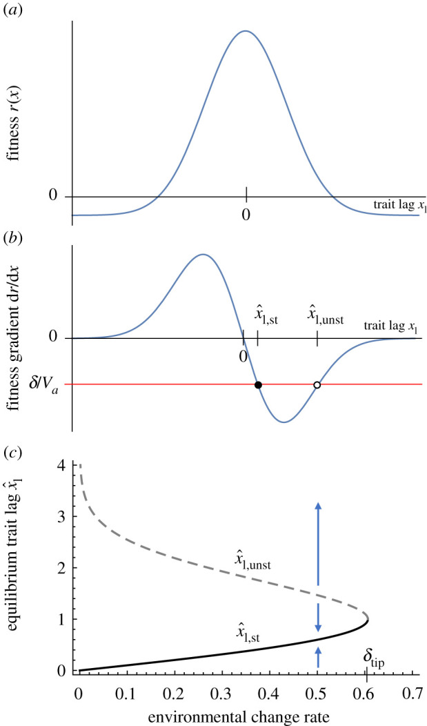
Non-quadratic fitness landscapes. (a) A Gaussian fitness landscape. (b) The fitness gradient has extrema at the inflection points of the fitness landscape, so that the rate of adaptation does not increase linearly with trait lag. (c) Depending on the rate of environmental change δ and the additive genetic variance Vg, this results in either two equilibria, one stable (solid line) and one unstable (dashed line), or no equilibrium at all when δ > δtip. Parameter values: rmax = 1, σr = 1, d = 0.1, Vg = 1. (Online version in colour.)
Evolutionary tipping points have also been observed in a recent extension of the moving optimum model to stage-structured populations [14]. This is despite the fact that each component of fitness in this model is quadratic (in continuous time). However, in age- and stage-structured populations the selection gradient (and thus life-time fitness) depends on the elasticities of each transition [15], which vary with mean trait value, creating nonlinearities. These nonlinearities can then cause extrema in the selection gradient, just as inflection points in the fitness function do (see also Complication 2: population dynamics (§4)).
4. Complication 2: population dynamics
Perhaps the biggest simplification of many quantitative genetics moving optimum models is ignoring density dependence by assuming exponential growth. These models assume that a population persists when fitness is positive, and goes extinct when fitness is negative, , and that this fitness function does not change with density. However, a basic ecological tenet is that exponential growth cannot be maintained indefinitely: at some point, population growth (and fitness) becomes density-dependent. A number of studies have therefore included density dependence in analytical explorations of moving optimum models (e.g. [11,16,17]), and essentially all simulations of the moving optimum model have required at least a simple carrying capacity to be computationally feasible.
One straightforward way to include density dependence is to allow fitness to be a function of population density, N. Then demography and evolution can be combined by augmenting the dynamics of the mean trait (equation (2.2)) with population dynamics given by . This approach has been called ‘ecological quantitative genetics' to emphasize its coupling of ecological and evolutionary dynamics on similar timescales [18]. It is closely related to the eco-evolutionary framework of adaptive dynamics [19]. However, unlike adaptive dynamics, ecological quantitative genetics does not assume that evolution is mutation-limited [18], making it more appropriate for understanding persistence in rapidly changing environments.
The details of how fitness depends on population density and the trait under selection can have a major effect on the ability of evolution to allow persistence (see, for example, [17]). For example, consider the per capita growth rate of a population, which is the difference between births and deaths: . Density dependence and trait dependence (i.e. selection) can each enter into both of these terms. The following models all feature logistic density dependence, which prevents unlimited growth, and quadratic trait dependence of fitness, but in four different combinations:
| 4.1a |
| 4.1b |
| 4.1c |
| 4.1d |
Trait dependence occurs in the birth term of equations (4.1a) and (4.1c) and the death term of equations (4.1b) and (4.1d). By contrast, density dependence affects deaths in equations (4.1a) and (4.1d) and births in equations (4.1b) and (4.1c). Of course, these four combinations can occur together; we consider them separately to illustrate the differences among them. All of these fitness functions match the density-independent quantitative genetics model (2.1) at low densities (), which is particularly relevant for population persistence. Note that populations are driven extinct before birth rates can become negative in (4.1a) and (4.1c). We find equilibrium population size and trait lag by setting and and solving for and [20].
All of these models share the same critical rate of change , where at the equilibrium trait lag , as in traditional quantitative genetics models. However, they show different patterns of equilibrium population size and trait lag as the rate of environmental change increases (figure 3). When density dependence and trait dependence are independent (equations (4.1a) and (4.1b)), the trait lag increases linearly and the population size declines quadratically with until (figure 3a; as shown in Figure 2D,E in [17]). These two equations are formally identical, so they behave the same way. When births depend on both density and the trait, the trait lag increases faster initially while population size declines approximately linearly (figure 3b; see Figure 3D,E in [17], where the only difference is that birth rate is Gaussian rather than quadratic). Most interestingly, when deaths depend on both density and the trait, populations can persist for , albeit in a bistable state, up to an evolutionary tipping point at (figure 3c).
Figure 3.

Interaction between density dependence (DD) and trait dependence (TD) of fitness. (a) When density and trait dependence enter different terms, they do not interact and the equilibrium trait lag increases linearly with δ. (b) When births are both density- and trait-dependent, the equilibrium trait lag increases nonlinearly with δ but results in the same critical value δc. (c) When deaths are both density- and trait-dependent, the species may continue to persist for δc < δ < δtip with two stable equilibria (solid lines), separated by an unstable equilibrium (dashed line). Parameter values: dmin = 0.1 or d = 0.1, bmax = 1 or b = 1, σr = 1, Vg = 1. (Online version in colour.)
What causes this bistability in the case of density- and trait-dependent deaths? We can answer this question using the eco-evolutionary phase plane, which shows the dynamics as a function of N and [20]. The interaction between density dependence and selection bends the -isocline to the left, making multiple intersections with the -isocline possible (figure 4; see other phase plane diagrams in electronic supplementary material, figure S1). Biologically, this can be understood as a positive feedback between population density and selection. Because selection occurs through deaths, at high population densities selection is stronger, enabling a smaller trait lag, which keeps the population high. If the population became small, it would experience less density-dependent mortality. This would relax selection, causing the trait to lag further behind the optimum and the population to diminish further, resulting in an ‘existential crisis'. Note that if the density and trait dependence of fitness instead works through births, the feedback is negative: increased population density would result in fewer births, which would weaken the strength of selection (electronic supplementary material, figure S1C). See figure 1 in [17] for a depiction of these pathways and [21] for further discussion on the interaction between life-history and persistence.
Figure 4.

Eco-evo phase plane analysis of density- and trait-dependent death model. (a) For δ < δc, there is a single stable equilibrium (filled circle) where the species persists. (b) For δc < δ < δtip, there are two stable equilibria (persistence and extinction) separated by an unstable equilibrium (open circle). (c) For δ > δtip, only the extinction equilibrium is stable. Other parameter values as in figure 3.
Therefore, even in these simple models, the potential for evolutionary rescue rests on the details of how fitness depends on density and traits. Understanding these effects in organisms with more complex life cycles remains an important open question. Other kinds of population dynamics also need to be explored; for example, populations that have ecological multiple stable states owing to Allee effects are likely to also possess evolutionary tipping points in changing environments.
5. Complication 3: community context
Species do not exist in isolation. Interactions between species, such as competition, predation/parasitism and cooperation, can have dramatic effects on both the demography and selection of a focal population and are thus integral to the ability of a population to adapt and persist. Appropriately, a number of moving optima models have included competition [22–26] and predation [17,27,28]. On the other hand, we did not find any studies that model both a moving optimum and a mutualism (but see [29] for an example of within-species cooperation), suggesting a gap in our understanding that could be readily filled. These studies are briefly summarized in electronic supplementary material, table S1. In each of these three cases—competition, predation and cooperation—the interaction can either help or hurt the focal population's persistence, depending on a number of factors (e.g. whether a population is leading or lagging, which life-history stage the interaction affects, and how the interaction impacts effective population size). There are many more complications to be explored before we have a clear and comprehensive picture of how communities will adapt and reorganize in changing environments.
A disconnect between theory and experimentation also exists, considering community adaptation. Experiments that expose communities to environmental change typically impose abrupt, i.e. ‘press', environmental changes (e.g. [30–37]). Experiments that expose communities to gradual change (e.g. [38,39]) will be essential for testing the predictions summarized in electronic supplementary material, table S1, and inspiring future theory.
6. Complication 4: fundamental niche limits
A central assumption of most moving optimum models is that the fitness function maintains its shape while it shifts at a constant rate forever. That is, these models assume that there are no fundamental limits to either changes in the environmental conditions or the ability of organisms to adapt (figure 5a). While this facilitates model analysis using the moving-frame-of-reference approach, neither assumption is biologically or physically possible.
Figure 5.

Contrasting (a) the moving optimum paradigm with (b) finite fitness landscapes with bounded environmental change. In (a), indefinite species persistence occurs when the equilibrium trait lag is less than the critical lag. In (b), the species can persist without evolution when the final environmental condition Epost < Ec,eco, goes extinct even with evolution when Epost > Ec,evo and may or may not persist when Ec,eco < Epost < Ec,evo.
We present an alternative conceptual framework, similar to that of [28,40,41], in figure 5b. As in the classic quantitative genetics moving optimum models we assume a unimodal fitness landscape, , for a given environmental value E, but by contrast, the height of the landscape decreases with increasing E. This sets an upper limit to adaptation, , beyond which evolution is unable to rescue the species. This upper limit results from fundamental biological constraints, where adaptation is either impossible (or at least much slower than the rate of environmental change) or where the net benefits are negative. For example, while populations may be able to adapt relatively quickly to a few degrees of warming or a slight drop in pH, there may be much less genetic variance available (or possible) to adapt to extreme heat and acidity, imposing near fundamental limits on adaptation (e.g. [42]). The environmental tolerance of a species with fixed traits adapted to the pre-environmental-change environment, , represents the current fundamental niche and defines another critical environmental value, .
Including a fundamental limit to adaptation results in three possible cases for the potential of evolutionary rescue depending on the final post-environmental-change environment . If , then the species will persist even with no adaptation. If , then extinction is inevitable. These limits do not depend on the rate of environmental change, only its magnitude.
The situation with intermediate amounts of environmental change, , is more complicated. In this case, the outcome depends on the rate of environmental change relative to the rate of adaptation. If environmental change is sufficiently slow or there is abundant additive genetic variance, then population persistence is guaranteed (figure 6a,b), as in classic moving optimum models without fundamental niche limits. However, if environmental change is faster or additive genetic variance is lacking, then the trajectory of can leave the region where fitness is positive, (figure 6c). Once fitness becomes sufficiently negative, the population size plummets. The situation is then more akin to an abrupt environmental change, where a large amount of theory has explored the probability of persistence (reviewed in [43] and [1]; for quantitative traits see, for example, [44–48]). Novel mathematical techniques such as rate-dependent bifurcation theory [49] may be useful tools for analysing models with non-uniform environmental change that cannot be transformed into moving-frame-of-reference.
Figure 6.

When Ec,eco < Epost < Ec,evo, persistence depends on the amount of additive genetic variance Vg relative to the rate of environmental change. (a) When change is slow relative to the rate of adaptation, fitness remains positive and the population maintains a high abundance. (b) For smaller genetic variance, the transient trait lag increases, putting populations at risk. (c) When the trait lag leaves the region of positive growth, the population can reach low densities where demographic stochasticity may drive it extinct. Fitness function r(x,E) = 1−(x−E)2−0.75E, environmental dynamics E(t) = 6(δt)5−15(δt)4 + 10(δt)3 for δt < 1 and E(t) = Epost = 1 for δt < 1. Mortality is density-dependent. Parameter values: δ = 0.1, d = 0.1.
7. Conclusion
Fitness landscapes have been a central concept in evolutionary theory [50]. Most classical quantitative genetics moving optimum models have assumed a density-independent quadratic fitness function whose shape remains invariant as it neverendingly shifts at a constant rate (figure 5a). These simplifying assumptions have facilitated mathematical analysis but limit the ecological realism of these models. We have shown that when the fitness function has inflection points (Complication 1) or there are interactions between density and trait dependence (Complication 2), there may be evolutionary tipping points where populations experience ‘existential crises'. Interspecific interactions (Complication 3) can further complicate the picture, either enhancing or inhibiting adaptation and persistence. Finally, fundamental limits to adaptation (Complication 4, figure 5b) may be the primary determinant of whether evolution can allow species to persist in changing environments in the long run. Moving optimum theory has focused on the rate of environmental change, yet this rate is likely only important for persistence when the final environmental state, , exceeds a species' current tolerance limit, , but is less than the evolutionary limit, (figure 6). Therefore, in an ecological context, fitness landscapes are multidimensional, depending not only on the distance between a trait and its optimum, but on the absolute value of the environmental variables, as well as intraspecific population density and community context.
While here we considered several aspects of ecological realism, many more aspects remain unexplored. A fruitful research direction would be to put the concept of evolutionary rescue in a more ecologically rich context and develop theory and experiments that would comprehensively address realistic scenarios. Mapping multidimensional fitness functions will involve extensive observational and experimental work guided by organismal-level theory such as dynamic energy budget models [51] and combined with the community ecological theory of species interactions [52,53]. The nonlinearity of the genotype–phenotype map presents an additional challenge to applying quantitative genetics models to evolutionary rescue [54]. Future studies that transplant populations and manipulate environmental conditions will help probe the tails of fitness functions, which can be fitted by nonparametric functions instead of assuming quadratics [55].
Empirically, evolutionary rescue has been demonstrated in many taxa [1]. Evolution experiments show that species can adapt to changing conditions, including global change stressors. Trait means shift towards values that better match new environmental conditions. For example, in marine phytoplankton, higher temperatures lead to the evolution of higher temperature optima and higher maximum temperatures at which growth is possible [56]. In fruit flies, higher temperatures also led to the selection of more thermally tolerant genotypes [57]. However, some recent experimental studies showed that there are limits to evolutionary rescue. Resource limitation prevented adaptation to higher temperatures in marine phytoplankton, likely because thermal tolerance depended on resource availability. Introducing this complication into an eco-evolutionary model generated predictions that matched the observed empirical patterns [58]. Predicting species persistence in changing environments requires approaches that link theory and empirical work and integrate across biological scales from organisms to communities.
Supplementary Material
Supplementary Material
Supplementary Material
Acknowledgements
We thank Helmut Hillebrand for organizing the HIFMB symposium and the special issue, Jon Chase and Stan Harpole for discussions, and two anonymous reviewers for helpful comments.
Data accessibility
The Mathematica code used in this paper is included for review as electronic supplementary material.
Authors' contributions
C.A.K. coded the models. All authors contributed to writing the manuscript.
Competing interests
We declare we have no competing interests.
Funding
This research was supported by NSF grants nos. DEB-1136710, DEB-1754250, OCE-1638958 and a grant from the Simons Foundation. C.A.K. and E.L. were supported by fellowships from the German Centre for Integrative Biodiversity Research, and M.M.O. was supported by the Center for Population Biology (UC Davis) and Banting (Canada) Postdoctoral Fellowships. This is KBS publication number 2167.
References
- 1.Bell G. 2017. Evolutionary rescue. Annu. Rev. Ecol. Evol. Syst. 48, 605–627. ( 10.1146/annurev-ecolsys-110316-023011) [DOI] [Google Scholar]
- 2.Radchuk V, et al. 2019. Adaptive responses of animals to climate change are most likely insufficient. Nat. Commun. 10, 3109 ( 10.1038/s41467-019-10924-4) [DOI] [PMC free article] [PubMed] [Google Scholar]
- 3.Kopp M, Matuszewski S. 2014. Rapid evolution of quantitative traits: theoretical perspectives. Evol. Appl. 7, 169–191. ( 10.1111/eva.12127) [DOI] [PMC free article] [PubMed] [Google Scholar]
- 4.Aitken SN, Yeaman S, Holliday JA, Wang T, Curtis-McLane S. 2008. Adaptation, migration or extirpation: climate change outcomes for tree populations. Evol. Appl. 1, 95–111. ( 10.1111/j.1752-4571.2007.00013.x) [DOI] [PMC free article] [PubMed] [Google Scholar]
- 5.Willi Y, Hoffmann AA. 2009. Demographic factors and genetic variation influence population persistence under environmental change. J. Evol. Biol. 22, 124–133. ( 10.1111/j.1420-9101.2008.01631.x) [DOI] [PubMed] [Google Scholar]
- 6.Gienapp P, Lof M, Reed TE, McNamara J, Verhulst S, Visser ME. 2013. Predicting demographically sustainable rates of adaptation: can great tit breeding time keep pace with climate change? Phil. Trans. R. Soc. B 368, 20120289 ( 10.1098/rstb.2012.0289) [DOI] [PMC free article] [PubMed] [Google Scholar]
- 7.Vedder O, Bouwhuis S, Sheldon BC. 2013. Quantitative assessment of the importance of phenotypic plasticity in adaptation to climate change in wild bird populations. PLoS Biol. 11, e1001605 ( 10.1371/journal.pbio.1001605) [DOI] [PMC free article] [PubMed] [Google Scholar]
- 8.Lynch M, Gabriel W, Wood AM. 1991. Adaptive and demographic responses of plankton populations to environmental change. Limnol. Oceanogr. 36, 1301–1312. ( 10.4319/lo.1991.36.7.1301) [DOI] [Google Scholar]
- 9.Lynch M, Lande R. 1993. Extinction and evolution in response to environmental change. In Biotic interactions and global change (eds Kareiva PM, Kingsolver JG, Huey RB), pp. 235–250. Sunderland, MA: Sinauer Associates. [Google Scholar]
- 10.Lande R. 1976. Natural selection and random genetic drift in phenotypic evolution. Evolution 30, 314–334. ( 10.1111/j.1558-5646.1976.tb00911.x) [DOI] [PubMed] [Google Scholar]
- 11.Bürger R, Lynch M. 1995. Evolution and extinction in a changing environment: a quantitative-genetic analysis. Evolution 49, 151–163. ( 10.1111/j.1558-5646.1995.tb05967.x) [DOI] [PubMed] [Google Scholar]
- 12.Osmond MM, Klausmeier CA. 2017. An evolutionary tipping point in a changing environment. Evolution 71, 2930–2941. ( 10.1111/evo.13374) [DOI] [PubMed] [Google Scholar]
- 13.Lande R, Arnold SJ. 1983. The measurement of selection on correlated characters. Evolution 37, 1210–1226. ( 10.1111/j.1558-5646.1983.tb00236.x) [DOI] [PubMed] [Google Scholar]
- 14.Cotto O, Sandell L, Chevin LM, Ronce O. 2019. Maladaptive shifts in life history in a changing environment. Am. Nat. 194, 558–573. ( 10.1086/702716) [DOI] [PubMed] [Google Scholar]
- 15.Barfield M, Holt RD, Gomulkiewicz R. 2011. Evolution in stage-structured populations. Am. Nat. 177, 397–409. ( 10.1086/658903) [DOI] [PMC free article] [PubMed] [Google Scholar]
- 16.Polechová J, Barton N, Marion G. 2009. Species’ range: adaptation in space and time. Am. Nat. 174, E186–E204. ( 10.1086/605958) [DOI] [PubMed] [Google Scholar]
- 17.Osmond MM, Otto SP, Klausmeier CA. 2017. When predators help prey adapt and persist in a changing environment. Am. Nat. 190, 83–98. ( 10.1086/691778) [DOI] [PubMed] [Google Scholar]
- 18.Klausmeier CA, Kremer CT, Koffel T. 2020 Trait-based ecological and eco-evolutionary theory. In Theoretical ecology: principles and applications (eds McCann KS, Gellner G), pp. 161–194, 4th edn Oxford, UK: Oxford University Press. [Google Scholar]
- 19.Geritz SAH, Kisdi É, Meszéna G, Metz JAJ. 1998. Evolutionarily singular strategies and the adaptive growth and branching of the evolutionary tree. Evol. Ecol. 12, 35–57. ( 10.1023/A:1006554906681) [DOI] [Google Scholar]
- 20.Otto SP, Day T. 2007. A biologist's guide to mathematical modeling in ecology and evolution. Princeton, NJ: Princeton University Press. [Google Scholar]
- 21.Orive ME, Barfield M, Fernandez C, Holt RD. 2017. Effects of clonal reproduction on evolutionary lag and evolutionary rescue. Am. Nat. 190, 469–490. [DOI] [PubMed] [Google Scholar]
- 22.de Mazancourt C, Johnson E, Barraclough TG. 2008. Biodiversity inhibits species' evolutionary responses to changing environments. Ecol. Lett. 11, 380–388. ( 10.1111/j.1461-0248.2008.01152.x) [DOI] [PubMed] [Google Scholar]
- 23.Johansson J. 2008. Evolutionary responses to environmental changes: how does competition affect adaptation? Evolution 62, 421–435. ( 10.1111/j.1558-5646.2007.00301.x) [DOI] [PubMed] [Google Scholar]
- 24.Norberg J, Urban MC, Vellend M, Klausmeier CA, Loeuille N. 2012. Eco-evolutionary responses of biodiversity to climate change. Nat. Clim. Change 2, 747 ( 10.1038/nclimate1588) [DOI] [Google Scholar]
- 25.Van Den Elzen CL, Kleynhans EJ, Otto SP. 2017. Asymmetric competition impacts evolutionary rescue in a changing environment. Proc. R. Soc. B 284, 20170374 ( 10.1098/rspb.2017.0374) [DOI] [PMC free article] [PubMed] [Google Scholar]
- 26.Thompson PL, Fronhofer EA. 2019. The conflict between adaptation and dispersal for maintaining biodiversity in changing environments. Proc. Natl Acad. Sci. USA 116, 21 061–21 067. ( 10.1073/pnas.1911796116) [DOI] [PMC free article] [PubMed] [Google Scholar]
- 27.Jones AG. 2008. A theoretical quantitative genetic study of negative ecological interactions and extinction times in changing environments. BMC Evol. Biol. 8, 119 ( 10.1186/1471-2148-8-119) [DOI] [PMC free article] [PubMed] [Google Scholar]
- 28.Mellard JP, de Mazancourt C, Loreau M. 2015. Evolutionary responses to environmental change: trophic interactions affect adaptation and persistence. Proc. R. Soc. B 282, 20141351 ( 10.1098/rspb.2014.1351) [DOI] [PMC free article] [PubMed] [Google Scholar]
- 29.Henriques GJB, Osmond MM. 2020. Cooperation can promote rescue or lead to evolutionary suicide during environmental change. Evolution 74, 1255–1273. ( 10.1111/evo.14028) [DOI] [PubMed] [Google Scholar]
- 30.Lawrence D, Fiegna F, Behrends V, Bundy JG, Phillimore AB, Bell T, Barraclough TG. 2012. Species interactions alter evolutionary responses to a novel environment. PLoS Biol. 10, 1001330 ( 10.1371/journal.pbio.1001330) [DOI] [PMC free article] [PubMed] [Google Scholar]
- 31.Tseng M, O'Connor MI. 2015. Predators modify the evolutionary response of prey to temperature change. Biol. Lett. 11, 20150798 ( 10.1098/rsbl.2015.0798) [DOI] [PMC free article] [PubMed] [Google Scholar]
- 32.Low-Décarie E, Kolber M, Homme P, Lofano A, Dumbrell A, Gonzalez A, Bell G. 2015. Community rescue in experimental metacommunities. Proc. Natl Acad. Sci. USA 112, 14 307–14 312. ( 10.1073/pnas.1513125112) [DOI] [PMC free article] [PubMed] [Google Scholar]
- 33.Gómez P, Paterson S, De Meester L, Liu X, Lenzi L, Sharma MD, McElroy K, Buckling A. 2016. Local adaptation of a bacterium is as important as its presence in structuring a natural microbial community. Nat. Commun. 7, 12453 ( 10.1038/ncomms12453) [DOI] [PMC free article] [PubMed] [Google Scholar]
- 34.Fugère V, et al. 2020. Community rescue in experimental phytoplankton communities facing severe herbicide pollution. Nature Ecol. Evol. 4, 578–588. ( 10.1038/s41559-020-1134-5) [DOI] [PubMed] [Google Scholar]
- 35.Bell G, Fugère V, Barrett R, Beisner B, Cristescu M, Fussmann G, Shapiro J, Gonzalez A. 2019. Trophic structure modulates community rescue following acidification. Proc. R. Soc. B 286, 20190856 ( 10.1098/rspb.2019.0856) [DOI] [PMC free article] [PubMed] [Google Scholar]
- 36.Limberger R, Fussmann GF. 2019. Adaptation and evolutionary rescue in a community context. bioRxiv, 734509 ( 10.1101/734509) [DOI] [Google Scholar]
- 37.Petkovic N, Colegrave N. 2019. Sex increases the probability of evolutionary rescue in the presence of a competitor. J. Evol. Biol. 32, 1252–1261. ( 10.1111/jeb.13525) [DOI] [PubMed] [Google Scholar]
- 38.Zhang Q-G, Buckling A. 2011. Antagonistic coevolution limits population persistence of a virus in a thermally deteriorating environment. Ecol. Lett. 14, 282–288. ( 10.1111/j.1461-0248.2010.01586.x) [DOI] [PubMed] [Google Scholar]
- 39.McTee M, Bullington L, Rillig MC, Ramsey PW. 2018. Do soil bacterial communities respond differently to abrupt or gradual additions of copper? FEMS Microbiol. Ecol. 95, fiy212 ( 10.1093/femsec/fiy212) [DOI] [PMC free article] [PubMed] [Google Scholar]
- 40.Pease CM, Lande R, Bull JJ. 1989. A model of population growth, dispersal and evolution in a changing environment. Ecology 70, 1657–1664. ( 10.2307/1938100) [DOI] [Google Scholar]
- 41.Ferriere R, Legendre S. 2013. Eco-evolutionary feedbacks, adaptive dynamics and evolutionary rescue theory. Phil. Trans. R. Soc. B 368, 20120081 ( 10.1098/rstb.2012.0081) [DOI] [PMC free article] [PubMed] [Google Scholar]
- 42.Belilla J, Moreira D, Jardillier L, Reboul G, Benzerara K, López-García JM, Bertolino P, López-Archilla AI, López-García P. 2019. Hyperdiverse archaea near life limits at the polyextreme geothermal Dallol area. Nature Ecol. Evol. 3, 1552–1561. ( 10.1038/s41559-019-1005-0) [DOI] [PMC free article] [PubMed] [Google Scholar]
- 43.Alexander HK, Martin G, Martin OY, Bonhoeffer S. 2014. Evolutionary rescue: linking theory for conservation and medicine. Evol. Appl. 7, 1161–1179. ( 10.1111/eva.12221) [DOI] [PMC free article] [PubMed] [Google Scholar]
- 44.Gomulkiewicz R, Holt RD. 1995. When does evolution by natural selection prevent extinction? Evolution 49, 201–207. ( 10.1111/j.1558-5646.1995.tb05971.x) [DOI] [PubMed] [Google Scholar]
- 45.Boulding EG, Hay T. 2001. Genetic and demographic parameters determining population persistence after a discrete change in the environment. Heredity 86, 313–324. ( 10.1046/j.1365-2540.2001.00829.x) [DOI] [PubMed] [Google Scholar]
- 46.Chevin LM. 2013. Genetic constraints on adaptation to a changing environment. Evolution 67, 708–721. ( 10.1111/j.1558-5646.2012.01809.x) [DOI] [PubMed] [Google Scholar]
- 47.Osmond MM, de Mazancourt C. 2013. How competition affects evolutionary rescue. Phil. Trans. R. Soc. B 368, 20120085 ( 10.1098/rstb.2012.0085) [DOI] [PMC free article] [PubMed] [Google Scholar]
- 48.Anciaux Y, Lambert A, Ronce O, Roques L, Martin G. 2019. Population persistence under high mutation rate: from evolutionary rescue to lethal mutagenesis. Evolution 73, 1517–1532. ( 10.1111/evo.13771) [DOI] [PubMed] [Google Scholar]
- 49.Ashwin P, Wieczorek S, Vitolo R, Cox P. 2012. Tipping points in open systems: bifurcation, noise-induced and rate-dependent examples in the climate system. Phil. Trans. R. Soc. A 370, 1166–1184. ( 10.1098/rsta.2011.0306) [DOI] [PubMed] [Google Scholar]
- 50.Svensson E, Calsbeek R. 2012. The adaptive landscape in evolutionary biology. Oxford, UK: Oxford University Press. [Google Scholar]
- 51.Kooijman SALM. 2010. Dynamic energy budget theory for metabolic organization. Cambridge, UK: Cambridge University Press. [Google Scholar]
- 52.Chase JM, Leibold M. 2003. Ecological niches: linking classical and contemporary approaches. Chicago, IL: University of Chicago Press. [Google Scholar]
- 53.Pásztor L, Botta-Dukát Z, Magyar G, Czárán T, Meszéna G. 2016. Theory-based ecology: a Darwinian approach. Oxford, UK: Oxford University Press. [Google Scholar]
- 54.Milocco L, Salazar-Ciudad I. 2020. Is evolution predictable? Quantitative genetics under complex genotype-phenotype maps. Evolution 74, 230–244. ( 10.1111/evo.13907) [DOI] [PubMed] [Google Scholar]
- 55.Schluter D. 1988. Estimating the form of natural selection on a quantitative trait. Evolution 42, 849–861. ( 10.1111/j.1558-5646.1988.tb02507.x) [DOI] [PubMed] [Google Scholar]
- 56.O'Donnell DR, Hamman CR, Johnson EC, Kremer CT, Klausmeier CA, Litchman E. 2018. Rapid thermal adaptation in a marine diatom reveals constraints and trade-offs. Glob. Change Biol. 24, 4554–4565. ( 10.1111/gcb.14360) [DOI] [PubMed] [Google Scholar]
- 57.Rodríguez-Trelles F, Tarrío R, Santos M. 2013. Genome-wide evolutionary response to a heat wave in Drosophila. Biol. Lett. 9, 20130228 ( 10.1098/rsbl.2013.0228) [DOI] [PMC free article] [PubMed] [Google Scholar]
- 58.Aranguren-Gassis M, Kremer CT, Klausmeier CA, Litchman E. 2019. Nitrogen limitation inhibits marine diatom adaptation to high temperatures. Ecol. Lett. 22, 1860–1869. ( 10.1111/ele.13378) [DOI] [PubMed] [Google Scholar]
Associated Data
This section collects any data citations, data availability statements, or supplementary materials included in this article.
Supplementary Materials
Data Availability Statement
The Mathematica code used in this paper is included for review as electronic supplementary material.