

Abstract
The Pyrococcus horikoshii amino acid transporter GltPh revealed, like other channels and transporters, activity mode switching, previously termed wanderlust kinetics. Unfortunately, to date, the basis of these activity fluctuations is not understood likely due to a lack of experimental tools that directly access the structural features of transporters related to their instantaneous activity. Here, we take advantage of HS-AFM, unique in providing simultaneous structural and temporal resolution, to uncover the basis of kinetic mode switching in proteins. We developed membrane extension membrane protein reconstitution (MEMPR) that allows the analysis of isolated molecules. Together with localization AFM, principal component analysis, and hidden Markov modeling, we could associate structural states to a functional timeline, allowing to solve six structures from a single molecule, and to determine an inward-facing state (IFS), IFSopen-1, as a kinetic dead-end in the conformational landscape. The approaches presented on GltPh are generally applicable and open possibilities for time-resolved dynamic single-molecule structural biology.
Introduction
GltPh is a widely studied archaeal homologue of excitatory amino acid transporters (EAATs)1,2. These transporters are homotrimers of functionally independent protomers, where peripheral transport domains are associated with a central scaffold- or trimerization-domain3 (Extended Data Fig. 1a). Previous structural studies of GltPh transporter using X-ray crystallography and cryogenic electron microscopy (cryo-EM) have resolved a series of conformations within two major states: the outward-facing state (OFS, Extended Data Fig. 1b, top) and the inward-facing state (IFS, Extended Data Fig. 1b, bottom)3-14. The transition between these two major states mediates the co-transport of ions and an amino acid (3 Na+ and 1 Aspartate) across the membrane15. In EAATs, amino acid transport (e.g., Glutamate) is also coupled to H+ co-transport and K+ anti-port16. In the OFS, the transport domains adopt a conformation where they strongly protrude from the extracellular surface and where Asp and Na+ binding occurs. During a transport cycle, the OFS transport domain moves across the membrane, undergoing a vertical displacement with respect to the membrane plane, and transits into the IFS, where it protrudes from the cytoplasmic surface and where Asp and Na+ are released6. The substantial vertical transport domain motion coined the name ‘elevator mechanism’. The transporter can then, during a transport cycle, revert from IFS to OFS, free of substrate and ions. As a result of reversibility, the transporter can be observed in both states, either fully substrate-loaded or empty, shuttling back and forth across the membrane. Hence, it provides an excellent experimental system to study the transport mechanism structurally and kinetically. During the functional cycle, the trimerization domain is thought to remain statically anchored in the membrane, exposing only minor protrusion on the cytoplasmic membrane surface. Consequently, and relevant for the analysis of the transporter by high-speed atomic force microscopy (HS-AFM)17,18, only the OFS transport domains can be observed on the extracellular side (Extended Data Fig. 1c, top), while the IFS transport domains and the trimerization domain are visible on the cytoplasmic side (Extended Data Fig. 1c, bottom).
In addition to the vertical ‘elevator’ movement, cryo-EM structures revealed lateral displacements of the transport domains relative to the trimerization domain in the IFS, termed IFSopen (Extended Data Fig. 1b, bottom, Extended Data Fig. 1c, IFS open) and IFSclosed (Extended Data Fig. 1, IFS closed)4,5,8,10,19 . IFSopen and IFSclosed differ from each other regarding their inter-domain orientations and distances as well as the positions of the gating hairpin (HP, Extended Data Fig. 1b, inset), where IFSopen is the state from which substrate is released. The most striking structural feature that distinguishes the IFSopen and IFSclosed conformations (from a perspective that is later important for HS-AFM analysis) is the height difference between the transport domain and the trimerization domain: In IFSopen, the transport domain protrudes ~ 1.5 Å from the trimerization domain on the cytoplasmic side, while in the IFSclosed conformation, the height difference increases to ~ 5 Å. For comparison, the OFS transport domain is ~ 10 Å lower than the trimerization domain on the cytoplasmic side, entirely buried in the membrane. In general, OFSopen and OFSclosed conformational transitions involve much smaller domain movement as compared to IFSopen and IFSclosed, mostly limited to the opening of the gating element comprised of a helical hairpin (HP2) (Extended Data Fig. 1b, top, Extended Data Fig. 1c, OFS closed and OFS open).
The ‘elevator’ movement dynamics of the transport domains have been studied earlier using single-molecule Förster resonance energy transfer (smFRET) experiments by tracking the distance changes between two fluorophores on neighboring protomers of the trimer19-22. While such experiments provided unprecedented insights into molecular dynamics, they make use of fluorophores covalently grafted to the protein and provide rather indirect 1D (one-dimensional) distance measurements as a reporter of complex 3D conformational dynamics in proteins. Such experiments have reported that GltPh switched kinetic modes, with protomers being highly active and then silent for extensive periods of time22,23, as had been reported for other channels and transporter24-29, but failed to uncover the grounds of such kinetic behavior. Such changes between dynamic modes have formerly been termed ‘wanderlust kinetics’24 but eluded so far investigation since researchers lacked a methodology to report concomitantly the structural and functional state of a protein along its lifetime trace.
The GltPh ‘elevator’ movement dynamics have also been studied directly using HS-AFM imaging30 and HS-AFM line-scanning (HS-AFM-LS) experiments31,32. These experiments revealed both the ‘elevator’ movement and the independence of the transport domains. However, several aspects of these experiments could be improved: All former HS-AFM and HS-AFM-LS measurements were performed on transporters exposing the extracellular face, which precluded the identification and classification of the IFS substates, IFSopen and IFSclosed. In addition, the former experiments were performed on densely packed transporters, which was thought to be generally required for high-resolution HS-AFM imaging. However, the dense packing may introduce an additional problem: Protein function may be energetically impacted by direct protein-protein contacts, through electrostatic interactions at short distances, or through membrane-mediated interactions with an effective range up to ~ 10 nm33-35. Here, to overcome these limitations and eliminate disturbances from neighboring proteins, we report a membrane protein preparation method that we term membrane extension membrane protein reconstitution (MEMPR), which allows acquiring high-resolution HS-AFM imaging data of isolated, individual membrane reconstituted GltPh trimers, while preserving their ability to undergo conformational dynamics. This method allows the study of isolated GltPh transporter trimers from both the extracellular and the cytoplasmic faces, and the tracking of the real-time structural dynamics of all protomers simultaneously in an extended lipid bilayer with unprecedented detail. In addition, we developed a principal component analysis (PCA) based method that allows building energy landscapes of the transport domain states, which revealed several additional local minima within IFSopen and IFSclosed, namely IFSopen-1, IFSopen-2, IFSclosed-1, IFSclosed-2, and IFSclosed-3. Combining the structural and temporal information, we analyzed their interconversion pathways and parsed out a conformational state, IFSopen-1, with certain structural features of IFSclosed, which appears to be a kinetically locked state. Further, hidden Markov modeling (HMM)36,37 corroborated that a single hidden state accessible from the IFSopen conformational space can explain the experimentally observed ‘wanderlust kinetics’ in GltPh. The approaches described here represent a generally applicable pipeline for single-molecule structure-function analysis and allow us to calculate six structures of conformational states adopted over time by a single molecule.
Results
Tracking isolated membrane transporters at high-resolution
To track the real-time structural dynamics of GltPh protomers at high resolution using HS-AFM, we reconstituted GltPh into membranes consisting of 1,2-dioleoyl-sn-glycero-3-phosphocholine (DOPC), 1,2-dioleoyl-sn-glycero-3-phosphoethanolamine (DOPE) and 1,2-dioleoyl-sn-glycero-3-phospho-L-serine (DOPS) at ratio 8:1:1 (w:w:w) (Fig. 1, step 1, sample reconstitution). Negative-stain EM, allowing fast characterization of the reconstituted proteo-liposomes, revealed vesicles of ~ 50 – 100 nm in diameter densely packed with transporters, as expected following reconstitution at low lipid-to-protein ratio (LPR) of 0.7 (w:w) (Extended Data Fig. 2). Direct HS-AFM observation of the reconstituted proteo-liposomes confirmed the dense packing of GltPh trimers in the membrane, with ~ 90% coverage of the membrane area (Extended Data Fig. 3), consistent with previous observations30,31. To separate GltPh trimers from each other, we mixed the densely packed proteo-liposomes with empty liposomes and added 1x critical micelle concentration (CMC) of dodecyl-β-D-maltoside (DDM) to the mixture (Fig. 1 step 2, pre-physisorption mixture). This process transformed the proteo-liposomes into membrane sheets with surface areas ~ 104 – 105 nm2 (Extended Data Fig. 4). Comparing the surface areas of the membrane sheets (Fig. 1 step 2) to the reconstituted proteo-liposomes with areas ~ 103 – 104 nm2 as estimated from their diameter (Fig. 1 step 1), we expected that the protein density in these membranes was diluted ~ 5 – 10-fold to ~ 10 – 20% membrane coverage. Finally, following the physisorption of these membranes to the HS-AFM sample surface, the detergent was rinsed out through extensive buffer exchange – 5x complete buffer volume removal and replenishing – to complete the sample preparation (Fig. 1 steps 3 and 4). We measured droplet angles and found that the final sample is indistinguishable from a detergent-free solution (Extended Data Fig. 5). It can, however, not be excluded that traces of detergent remain in the membrane throughout the entire sample preparation process that takes typically tens of minutes until the beginning of HS-AFM imaging.
Figure 1 ∣. Workflow for the membrane extension membrane protein reconstitution (MEMPR) method for HS-AFM study of membrane protein structure and dynamics.

Step 1: Reconstituted proteo-liposomes of densely packed GltPh (see Methods). Step 2: Pre-physisorption mixture of reconstituted GltPh proteo-liposomes and empty liposomes plus 1x CMC detergent (DDM): ~15 min of mixture incubation before physisorption. Step 3: Physisorption of the mixture to the HS-AFM imaging sample surface, i.e., freshly cleaved mica. Pre-treatment of the mica with poly-Lys (mica coating) is optional: On mica: study of diffusive proteins and protein-protein interactions. On poly-Lys: study of immobilized protein and conformational dynamics (see Step 5). Step 4: Buffer exchange following the sample physisorption. The non-physisorbed sample and bulk of the pre-physisorption mixture is removed with a pipette and exchanged > 5 times with equal volume of detergent free imaging buffer (the sample is never allowed to dry during this step, ~ 1/32x CMC detergent). Step 5: HS-AFM imaging, of freely diffusing (5a) or immobilized (5b) GltPh molecules. Step 5b requires pre-treatment of the mica with poly-Lys in Step 3 (~ 1/1500x CMC detergent, Extended Data Fig. 5). All schematics were generated using Biorender.com.
The extension of the membrane over the entire sample surface liberated individual GltPh trimers from the dense molecular packing and provided space for them to diffuse (Fig. 1 step 5a). While fast-diffusing molecules resulted in transient topography streaks in scan lines, slow-diffusing and immobile molecules were resolved as trimers in HS-AFM imaging (Extended Data Fig. 6a, Supplementary Movie 1). Interestingly, some GltPh molecules diffused together as dimers-of-trimers, indicating substantial protein-protein interactions between GltPh trimers. In addition, stable 2D-clusters of GltPh trimers, ~ 5×10² – 5×10³ nm2 in size (comprising ~ 5 – 50 molecules given that each GltPh occupies ~ 100 nm2), were observed in the continuous membrane (Extended Data Fig. 6b,c, Supplementary Movies 2,3, Supplementary Note 1). These results generally agree with the in vivo observations of cluster formations of EAATs38,39.
While this protocol allows for visualizing the 2D-cluster dynamics of GltPh molecules, tracking the conformational states and transitions of individual trimers (Fig. 2a) requires immobilizing the molecules. To this end, we pretreated the HS-AFM imaging stage40, i.e., freshly cleaved mica, with poly-L-lysine (poly-Lys) at a low concentration of ~ 1 – 2 poly-Lys molecules (MW 4.7 kD, degree of polymerization = 30) per nm2, estimated at a 100% efficient poly-Lys physisorption to the mica (Fig. 1 step 5b). Thus, the employed density of poly-Lys only permitted the formation of a poly-Lys monolayer on the surface. As a result, GltPh molecules in the extended lipid bilayer spread on top of the poly-Lys monolayer displayed limited lateral mobility (Fig. 2b, Extended Data Fig. 7, Supplementary Movies 4-6). Besides permitting single-molecule imaging of isolated transporters, the poly-Lys layer held another advantage by providing a hydrophilic buffer-immersed cushion between the solid mica support and the protein-containing supported lipid bilayer (Fig. 1, step 5b). Depending on the imaging region, ~ 10 – 30% of the area was covered by molecules, matching the estimation of the protein density in the membrane. In the example region (Fig. 2b), ~ 15% of the immobilized GltPh were individual trimers, ~ 15% were in dimers-of-trimers, and ~ 70% of the trimers were found in higher-order clusters (Supplementary Note 1).
Figure 2 ∣. Single-molecule structural dynamics of GltPh in extended lipid bilayers by HS-AFM.
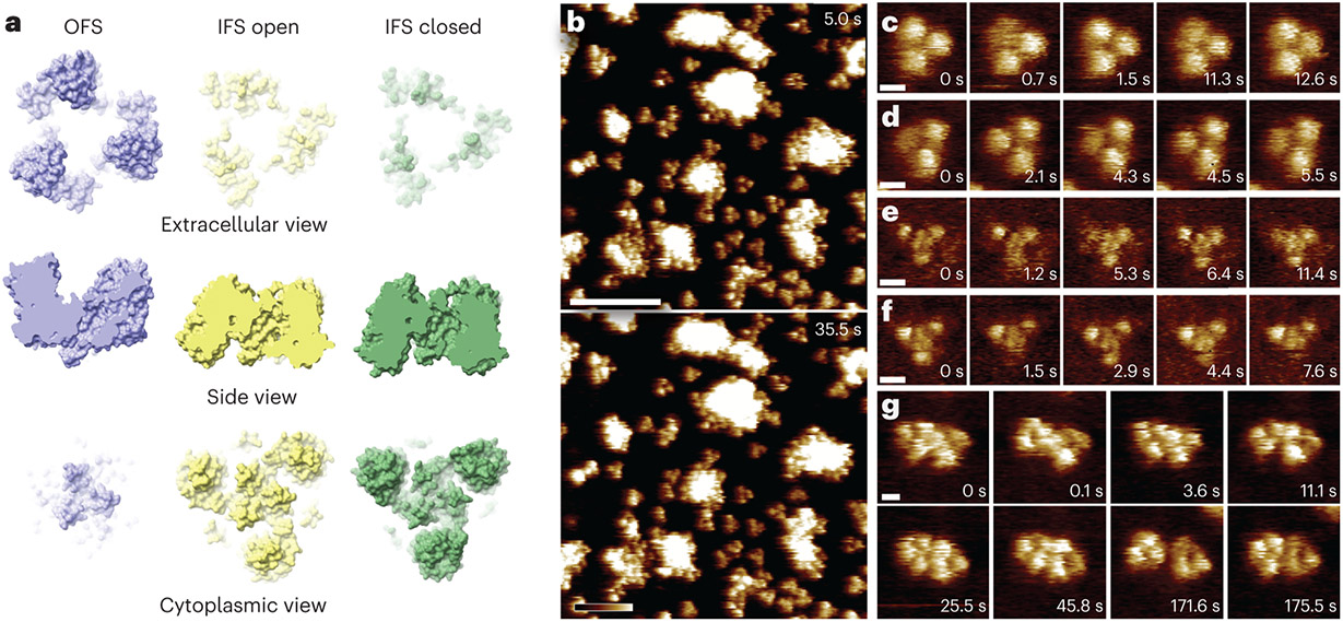
(a) PDB structures of GltPh in the outward-facing (OFS, blue, PDB: 6x17), inward-facing open (IFSopen, yellow, PDB: 6x12), and inward-facing closed (IFSclosed, green, PDB: 4p19) states. The structures are presented from the extracellular side (top), in a side view (middle), and from the cytoplasmic side (bottom), see also Extended Data Fig. 1. (b) HS-AFM frames (Supplementary Movie 4) of GltPh molecules in an extended lipid bilayer (image parameters: 1 nm/pixel, 0.5 s/frame) immobilized through pre-incubation of the underlying mica surface with poly-Lys. (c) to (f) HS-AFM frames (Supplementary Movies 7-10) of individual GltPh trimers viewed from the extracellular side (c) and (d), and from the cytoplasmic side (e) and (f) (image parameters: 0.25 nm/pixel, 0.1 s/frame). Individual protomers periodically interchanged between two states through the vertical displacement of the transport domain with a height difference of ~ 1 nm. These movements were visible at t = 0.7s in (c); t = 0.0s, 4.3s, and 5.5s in (d); t = 1.2s, 5.3s, and 11.4s in (e); And t = 1.5s and 7.6s in (f). The central trimerization domain is resolved as a small trefoil topography close to the 3-fold axis when viewed from the cytoplasmic side (e) and (f). (g) HS-AFM frames (Supplementary Movie 11) of a dimer of GltPh trimers from the extracellular side (image parameters: 0.5 nm/pixel, 0.1 s/frame). HS-AFM captured rotations, rearrangements, as well as ‘elevator’ movements of the individual transport domains (t = 11.1s, 45.8s, 171.6s, and 175.5s). The dimer-of-trimers had a center-to-center distance of 8.9 0.8 nm (mean s.d., n = 1757) while in close contact, but could be separated up to ~ 11 nm (t = 171.6 s), during ~ 1% of the imaging period. Similar lateral dynamics were observed between molecules in clusters (Extended Data Fig. 7c, arrowheads). Consistent results were obtained from > 3 HS-AFM experiments and > 3 reconstitution samples.
Excitingly, many individual GltPh trimers were completely isolated from other molecules (Fig. 2b), separated by free membrane resulting in > 8 nm edge-to-edge distance to their closest neighbors, and thus were free of membrane-mediated protein-protein disturbances33. This condition allowed stable tracking of single transport domain structural dynamics with unprecedented resolution, 0.1 s/frame and 0.25 nm/pixel in the example experiments, and stability, up to several minutes (Fig. 2c-f, Supplementary Movies 7-10). Furthermore, as an additional advantage of the MEMPR method, both the extracellular (Fig. 2c,d) and cytoplasmic (Fig. 2e,f) faces of GltPh were observed. In contrast, due to uniform membrane insertion, previous HS-AFM studies of densely packed GltPh imaged only the extracellular face. Although fixed in place, the molecules retained protomer dynamics, as ‘elevator’ movements of the transport domains were frequently observed (Fig. 2).
GltPh that formed dimers-of-trimers displayed increased lateral dynamics as compared to individual trimers (Fig. 2g, Supplementary Movie 11). This might be due to disturbances of each molecule by the activity of the neighbor, in other words, each trimer in the dimer-of-trimers not only displays its own inherent activities but also experiences the fluctuations from the neighbor. Therefore, for detailed analyses of single-molecule structural dynamics, it is necessary to target isolated GltPh trimers with a center-to-center distance > 18 nm (edge-to-edge distance > 10 nm) to their closest neighbors (Fig. 2c-f).
Elevator dynamics of single GltPh transport domains
For the subsequent analysis of the conformational dynamics, we chose molecules that exposed the cytoplasmic face to the HS-AFM tip (Fig. 2e,f) for three reasons: (i) All prior analyses were performed on molecules exposing the extracellular face. (ii) The trimerization domain, which is only visible from the cytoplasmic side, is stable in the membrane and can therefore serve as a reference point in analyzing the transport domain movements. (iii) Previous cryo-EM studies reported two distinct conformational substates of the IFS in the apo condition, IFSclosed and IFSopen (Fig. 2a)4,8, but their kinetics remained poorly explored. Investigating the transitions between these IFS substates and their transitions to/from the OFS requires imaging from the cytoplasmic side.
The first analysis concerned a two-state model, the ‘elevator’ interconversion between OFS and IFS only (Fig. 3, see also Fig. 2e). In this HS-AFM movie recorded at 10 frames per second (Supplementary Movie 9), the dynamics of a GltPh trimer was observed over 342 frames, providing a total of 1026 protomer-observations (POs) with time-protomer index for protomer in frame (Fig. 3a). To classify individual POs to different conformations, we assessed their pixel height distributions (Fig. 3b). The POs in the example molecule had a membrane-protruding height and a membrane-protruding volume (mean ± s.d., n = 1026). We applied the 2D Gaussian mixture model (Methods) to classify the POs into two clusters: and (Fig. 3c). Remarkably, POs in cluster of the total observations (n = 114), had smaller membrane protrusions, and (mean ± s.d.), than those in cluster (n = 912), and (mean ± s.d.). The POs distribution (Fig. 3c) could be transformed into a probability density map by assessing the abundance of data points at any location in the plot and, finally, by taking the ln of the probability density, into a free energy density plot (Fig. 3d, Methods). This plot provides an intuitive visual of the most favored conformation and the spread of the elevator motion of the transport domain between IFS and OFS for this molecule during the imaging period and under these experimental conditions.
Figure 3 ∣. Two-state structural dynamics of individual GltPh protomers.

(a) HS-AFM frames (Supplementary Movie 9) of an immobilized GltPh trimer (see Fig. 2f) in an extended lipid bilayer viewed from the cytoplasmic side. A total of 1026 POs with time-protomer index for protomer in frame were obtained. In frame 89, t89 (t = 8.8 s), the trimer had two OFS POs (t89p1 and t89p3) and one IFS PO (t89p2). (b) Height histograms of POs t89p1, t89p2, and t89p3. Red lines: 10% (, left) and 90% (, right) of the height values. (c) The vs (membrane protrusion volume vs height) distribution of all protomers from the GltPh molecule of interest (342 frames, n = 1026). OFS (blue, n = 114) and IFS (grey, n = 912) protomers were clustered using the 2D Gaussian mixture model (Methods). The locations of protomers t89p1, t89p2, and t89p3, shown in (b), are highlighted. (d) Energy landscape characterizing the OFS and IFS conformations of the molecule of interest, constructed from the protomer-observations (POs) distribution in (c). Dashed Lines: OFS and IFS clusters (e) Comparisons of the PDB structures (left), from the cytoplasmic view, and LAFM maps (right, Methods) of OFS (top) and IFS (bottom). The LAFM maps were calculated from all protomers in the corresponding states. (f) Two-state (IFS and OFS) conformation-time traces of individual protomers. (g) Left: GltPh IFS protomer distribution as a function of the temporal distance to their closest IFS-OFS transition activity (time to OFS). Right: LAFM maps calculated from ~ 250 IFS protomers, each pooled by their ‘time to OFS’ distance. IFSa1: time to OFS < 0.4 s. IFSa2: 0.4 – 1 s. IFSa3: 1.1 – 2.3 s. IFSa4: > 1.8 s. Relative rotation of the transport domain (arrow) and trimerization domain height as reference (asterisk) are indicated. The PCA and LAFM-based analysis workflow was successfully applied to > 3 single molecules from different reconstitution samples.
To assess the structural features of the POs in the different clusters in more detail, we applied the localization AFM algorithm (LAFM41, Methods) and constructed LAFM maps of the particles (protomers) in clusters (OFS) and (IFS) from the data points in Fig. 3c, respectively (Fig. 3e, right). In the OFS map, the trimerization domain protrudes further from the membrane than the transport domains (Fig. 3e, top). In contrast, in the IFS map, the transport domains protruded above the trimerization domain (Fig. 3e, bottom), in agreement with the cryo-EM structures (Fig. 3e, left). Indeed, the protrusion height difference between trimerization and transport domains appears to be an unambiguous method to classify observations into the two major states OFS and IFS, respectively (Fig. 3e).
Next, we combined for each PO the clustering result, i.e., what is the conformation, with the time of observation, i.e., when did this conformation occur, and reconstructed a two-state conformation-time trace of this GltPh trimer (Fig. 3f). Interestingly, while all three protomers favored IFS during the imaging period and under the current experimental conditions, protomer was substantially more active than the other two protomers, accounting for ~ 2/3 of the total OFS-IFS transitions. Consequently, protomers and presented longer dwell-times between adjacent OFS-IFS transitions, sometimes > 10 s. Thus, during the imaging period, was in a different kinetic mode than and . Switches between different kinetic modes in a single protomer were also observed in other molecules (Extended Data Fig. 8, Supplementary Movie 12), where a protomer spent ~ 20 s inactive in IFS, then ~ 40 s inactive in OFS, and then engaged for ~ 30 s in a highly active mode with intensive IFS-OFS transitions, slightly favoring OFS.
The observation of different kinetic modes, as has been formerly reported by smFRET19,20,22, led to other questions: What are the structural features that relate to the different activity modes? What is the structural state of a transporter when it is in a kinetically silent inactive state? We assumed that a protomer that is temporally closer to an IFS-OFS transition adopts more likely an active conformation. In contrast, conformations observed in the middle of an inactive period, temporally far away from any transition, should more likely represent a locked state. Hence, we calculated for all individual IFS POs (n = 912) their temporal distance to the closest IFS-OFS transition (Fig. 3g, left; time to OFS), where small ‘time to OFS’ values indicate transport domains that just recently were or are going to be active. Then, we calculated LAFM maps of four IFS PO groups as a function of increasing ‘time to OFS’ values (Fig. 3g, right): < 0.4 s for IFSa1 (active), 0.4 – 1 s for IFSa2 (intermediate active), 1.1 – 2.3 s for IFSa3 (intermediate inactive), and > 1.8 s for IFSa4 (inactive); where the pooling intervals were set to comprise identical numbers of POs (n = 250) to construct the LAFM maps. Excitingly, distinct structural features were revealed in these IFS LAFM maps, indicative of conformational signatures in IFS protomers that are relevant to their IFS-OFS activity. Specifically, the transport domains of active IFS protomers (IFSa1 and IFSa2) are ~ 3 Å higher than the inactive ones (IFSa3 and IFSa4), normalized to the trimerization domain. Besides the height reduction, the inactive transport domain had a counterclockwise rotation of ~ 15° as compared to the active protomers. These IFS LAFM maps (Fig. 3g, right) are directly comparable to the different IFS PDB structures, where similar transport domain height and rotation variations were reported4, but a deeper analysis of the conformational variability of the GltPh IFS protomers requires further classification of the IFS cluster POs (Fig. 4).
Figure 4 ∣. Three-state structural dynamics of individual GltPh protomers.

(a) HS-AFM frames (Supplementary Movie 9) of an immobilized GltPh trimer (see Fig. 2f) in an extended lipid bilayer viewed from the cytoplasmic side. In frame 1, t1 (0.0 s), all three POs (t1p1, t1p2, and t1p3) of the trimer were in IFS conformations, but with distinct structural features. (b) Height histograms of protomers t1p1, t1p2, and t1p3. These histograms were analyzed using principal component analysis (PCA) to extract features that allowed optimized classification of the IFS protomer characteristics (Methods). (c) Distribution of all IFS protomers (n = 912) in the space from the PCA. The pc1 and pc2 axes represent the two most significant features that provide the largest data spreading. Two clusters were identified as IFSopen (yellow) and IFSclosed (green) protomers from structural comparison. The locations of protomers t1p1, t1p2, and t1p3, shown in (b), are highlighted. (d) Energy landscape describing the IFS conformations of the molecule of interest, constructed from the protomer-observation distribution in (c). Dashed Lines: IFSopen and IFSclosed clusters. (e) Comparisons of the PDB structures (left), viewed from the cytoplasmic side, and the LAFM maps (right) of the OFS (top), IFSopen (middle), and IFSclosed (bottom) conformations (Methods). The LAFM maps were calculated from all protomers in the corresponding states, in (c). Relative rotation of the transport domain (arrow) and trimerization domain height as reference (asterisk) are indicated. (f) Selected HS-AFM frames and the corresponding states of individual protomers (colored schematics). White dashed circles: protomer locations. (g) Three-state (OFS, IFSopen, and IFSclosed) conformation-time traces of individual protomers. Color coding in (c), (f) and (g): OFS (blue), IFSopen (yellow), and IFSclosed (green). Similar results were observed in > 3 single-molecule analysis.
Classification of IFS open and IFS closed conformations
Although both IFSopen and IFSclosed conformations have transport domains that protrude further than the trimerization domain from the cytoplasmic side, the resolution in the HS-AFM movies readily revealed differences among the IFS POs (Fig. 4a, Supplementary Movie 9). For example, compared to protomers and , protomer protruded ~ 2 – 3 Å further, and its height distribution showed a long tail to larger values (Fig. 4b). Interestingly, protomer shared more similarity to than its predecessor () (Fig. 4a), indicating a transition event between two IFS conformations of protomer between and . Therefore, for a systematic classification of the IFS POs, we had to extract as many features as possible from the imaging data. To this end, we constructed a dataset of 912 IFS POs for this example molecule from which we extracted 8 image features from each PO (Fig. 4a, Methods).
Organizing a dataset with multiple variables is hard, primarily due to the high dimensionality of the data42: As the number of variables increases, the data become sparsely distributed in a space that grows exponentially with the variable number, thus undermining the efficiency of common data organization strategies such as clustering. Hence, it is necessary to seek a low-dimension representation with the most meaningful properties of the original high-dimensional data using dimension reduction tools. We thus applied principal component analysis (PCA)43 to the IFS PO dataset (Fig. 4c, Methods). The first two principal components ( and ) accounted for ~ 76% of the total data variance, i.e., 76% of the information in the dataset could be characterized with two numbers, sufficiently capturing the most representative intrinsic properties of the dataset. Excitingly, the IFS POs populated in two major clusters, (Fig. 4c, yellow data points, n = 624) and (Fig. 4c, green data points, n = 288), in the space. Again, to get a more intuitive representation of the conformational landscape, we plotted the data point distribution as a free energy density landscape (Fig. 4d).
LAFM maps of clusters (IFSopen, n = 624) and (IFSclosed, n = 288), displayed obvious structural differences in the protrusion height and the rotational localization of the transport domain with respect to the trimerization domain (Fig. 4e). Specifically, the transport domains in IFSopen are only ~ 2 Å higher than the trimerization domain, comparable to the estimated height difference of ~ 1.5 Å in the IFSopen conformation PDB structure (Fig. 4e, middle). In contrast, transport domains in IFSclosed are ~ 5 Å higher than the trimerization domain, matching the estimated height difference of ~ 5 Å in the IFSclosed conformation PDB structure (Fig. 4e, bottom). In addition to the height difference, we measured the relative orientations of the transport domains with respect to the trimerization domain in these LAFM maps. The transport domain peak positions in both LAFM maps are ~ 3 nm from the trimerization domain center, but in IFSclosed it is located ~ 20° clockwise with respect to its counterpart in IFSopen. These features in IFSopen and IFSclosed (Fig. 4e) were reminiscent of the features in the previously constructed IFS LAFM maps (Fig. 3g, IFSa1 to IFSa4). Hence, we concluded that IFS GltPh transport domains with high IFS-OFS activity (IFSa1 and IFSa2) were in an IFSclosed-like conformation, while those exhibiting low IFS-OFS activity and/or were kinetically locked (IFSa3 and IFSa4) adopted a conformation that was IFSopen-like (compare Fig. 4e, bottom and middle, to Fig. 3g, right).
Next, we combined the results from the IFSopen-IFSclosed clustering with the IFS-OFS clustering and assigned each PO in the example molecule (n = 1026) to either OFS, IFSopen or IFSclosed conformation (Fig. 4f), and constructed a three-state conformation-time trace for each of the three transport domains of this GltPh trimer (Fig. 4g). We found that the individual protomers were in different kinetic modes: Protomer favored the IFSclosed conformation and displayed high transmembrane IFS-OFS activity (mode CH, closed with high activity), while protomers and favored the IFSopen conformation during the imaging period and displayed low IFS-OFS activity (mode OL, open with low activity). The observation of these different kinetic modes, in both IFS-OFS and IFSopen-IFSclosed transitions, was indicative of a more complicated kinetic model with more conformational states.
More IFS conformation substates
In addition to the two major clusters, (IFSopen) and (IFSclosed) (Fig. 4c,d), we observed IFS PO sub-clusters within them. These sub-clusters were either defined by individual peaks with high local observation density (Fig. 5a, IFSclosed-1, IFSclosed-2) or as wide shoulders within a large density clearly hiding several Gaussians (Fig. 3a, IFSopen-1, IFSopen-2, IFSopen-3) in the space, indicative of more conformational variants of the GltPh IFS. Therefore, we constructed LAFM maps from ~ 100 POs near five locations with high local observation density in the space, two in (IFSclosed-1, IFSclosed-2) and three in (IFSopen-1, IFSopen-2, IFSopen-3) (Fig. 5a, insets).
Figure 5 ∣. IFSopen and IFSclosed conformational substates and identification of a kinetically trapped state.

(a) LAFM maps (insets) constructed from ~ 100 IFS protomer-observations (POs) localized in energy minima in the space conformational energy landscape, see Fig. 4d. Two conformational variants were resolved from the IFSclosed protomer cluster (IFSclosed-1 and IFSclosed-2), and three conformational variants from the IFSopen protomer cluster (IFSopen-1, IFSopen-2, and IFSopen-3). Relative rotation of the transport domain (arrowhead) and trimerization domain height as reference (asterisk) are indicated. (b) GltPh IFS POs colored by their temporal distances to the closest IFSclosed-IFSopen transition (time to IFSopen/IFSclosed). (c) Average local IFS GltPh activity map overlaid to the conformational energy landscape. Color: average local temporal distance to the closest transitions, either IFSclosed-IFSopen or IFS-OFS (time to all transitions). Black lines: iso-energy lines, modified from the conformational free energy map in (a).
The transport domains in the IFSclosed conformation variants resemble each other in their shape and relative orientation to the trimerization domain, except for a ~ 1 Å height difference. Specifically, the IFSclosed-1 protomers are ~ 5.5 Å higher than the trimerization domain, whereas the height difference is reduced to ~ 4.5 Å in IFSclosed-2. In contrast, larger structural variabilities were observed among the IFSopen conformation variants. Transport domains of IFSopen-2 and IFSopen-3 are ~ 1.5 Å higher than the trimerization domain, matching the estimated height difference of ~ 1.5 Å from the IFSopen PDB structure (Fig. 4e, IFSopen), but the height difference increases to ~ 2.5 Å in IFSopen-1. The peak protrusions of the transport domains in all three variants are ~ 3 nm away from the trimerization domain center, but the IFSopen-1 transport domain is located ~ 5° clockwise compared to its counterparts in the other two IFSopen conformation variants, closer to IFSclosed. These measurements of protomer heights and relative orientations indicated that IFSopen-1 shared some structural features with the IFSclosed conformations, while IFSopen-2 and IFSopen-3 resemble the canonical IFSopen conformation.
Next, like in the case of IFS-OFS transitions (Fig. 3g), we related these conformational variants to their IFSopen-IFSclosed activity by adding the time component to the PO distribution in the space (Fig. 5b). For individual IFS POs (n = 912), we measured their temporal distances to the closest IFSopen-IFSclosed transition (Fig. 5b, time to IFSopen-IFSclosed), and found that the POs in IFSclosed-1, IFSclosed-2, IFSopen-3 and IFSopen-2 had similar levels of activity. In contrast, interestingly, IFSopen-1 comprised > 50% of POs that were > 1 s away from an IFSopen-IFSclosed transition (Fig. 5b, dark data points). Therefore, our analysis suggested that, following an IFSclosed-IFSopen transition, the GltPh transport domains initially favor a canonical IFSopen conformation (IFSopen-2/IFSopen-3), however, they may enter a non-canonical IFSopen-1 conformation with several IFSclosed conformational features, which is inactive. While our HS-AFM LAFM map does not provide atomistic structural details, both the position and the protrusion height would predict that the transport domain was in a somewhat tilted orientation within the membrane, like in canonical IFSopen, but at a location closer to IFSclosed. Finally, we combined the IFS-OFS and IFSclosed-IFSopen activities and defined ‘time to all transitions’ as the smaller value of ‘time to OFS’ and ‘time to IFSopen-IFSclosed’. Using this value as an indicator of the activity of individual POs, we projected the average local protomer activity onto the IFS conformational free energy map (Fig. 5c). The average local activity map confirmed that IFSopen-1 is ~ 0.5 – 1 s farther away from all transitions as compared to other IFS variants and corresponds to an overall inactive conformation of IFS GltPh: A kinetic trap in its transport cycle. Comparison between IFSopen-1 and IFSa4 (from our two-state analysis) corroborates the structural features of the kinetically locked conformation.
Hidden Markov Model: A kinetic cul-de-sac in IFSopen
The hidden Markov model (HMM) has proven successful in understanding single-molecule dynamics data in various biophysics experiments44-47. An HMM describes a stochastic Markovian process in which the future state only depends on the current state, not on any previous information, with the possible existence of a set of unobservable (hidden) states, , as well as a set of observable outcomes, 36,37. Transitions among pairs of states in are described in the transition matrix , and the maps from to in the emission matrix (Supplementary Table 1, Methods).
In our study, is the intrinsic GltPh structures and is the measured three major conformational states (Fig. 4e, OFS, IFSopen, and IFSclosed). First, we considered a three-state model (model , Fig. 6a), in which each state maps specifically and exclusively to a measured outcome, i.e., . Thus, in model , the states are not ‘hidden’ from the outcomes but observable and exactly interpreted as outcomes, and its emission matrix is filled with ‘1’s in its main diagonal and ‘0’s elsewhere (Supplementary Table 1, Methods). The maximum likelihood estimate of the transition matrix that best characterized the observed conformation-time traces was then calculated using the Baum-Welch algorithm (Supplementary Table 1)48. In this model, all states are connected in . However, simulated outcome-time traces with and (Supplementary Table 1) expectedly fail to display multiple kinetic modes (Fig. 6a, right), in contrast to the experimental observations (Fig. 4g). Hence, to see kinetic switching emerge, ‘hidden’ states must be introduced to the model.
Figure 6 ∣. Hidden Markov models of the GltPh single transport domain conformation-time traces.

(a) and (b) HMMs proposed to interpret the experimentally observed conformation-time traces (see Fig. 4g). Model A (a) has a three-state structure (, , and ). Model B (b) has a four-state structure (), where is a hidden fourth state. Both models have three outcomes (, , and ) corresponding to the three major conformations, OFS (blue), IFSopen (yellow), and IFSclosed (green), respectively. Left: schematics of the HMMs. The colored pie chart next to state represents the emission probability distribution , reflecting the influence of state on all outcomes . The weighted arrows connecting state to all states represent its transition probability distribution at time-step to the next time-step . The probabilities are visualized as pie chart areas and arrow thicknesses (dashed lines: no transition), and details for the emission matrix , i.e., , and transition matrix , i.e., , can be found in supplementary table 1. Right: simulated three-state outcome-time traces for models A and B. Each trace has 1000 time-steps, equivalent to 100 s ( in this study). OL: IFS Open Low activity mode. CH: Closed High activity mode. Because state has 100% outcome (IFSopen), is conformationally similar to . Besides, both transitions from state to (100% outcome, OFS) and to (100% outcome, IFSclosed) have ~ 0% transition probability, indicating that state is exclusively connected to . State has a self-transition probability to of ~ 92%. These results revealed that two IFSopen states are present in model B, where state is active, but is quiescent with no kinetic transitions to other states.
To this end, we propose HMM model , in which we introduced an additional ‘hidden’ state, . Hidden state could potentially map to all other outcomes (Fig. 6b). The maximum likelihood estimate of the matrices indicated that the hidden state mostly resembled IFSopen (94% outcome, IFSopen, and 6% outcome, IFSclosed) and is quiescent with no kinetic transitions to other states (92% self-transition probability, Supplementary Table 1). The simulated outcome-time traces using model exhibited ‘wanderlust kinetics’ features, in which both modes and were observed and lasted for ~ 10 s. Model provides the kinetic basis for the existence of a hidden state, , which is both close and similar to IFSopen, that may account for the experimental findings. Comparing the IFSopen states in the experiments (Fig. 5a, IFSopen-1, IFSopen-2, and IFSopen-3) to those in the HHM model (Fig. 6b, and ), we conclude that should correspond to IFSopen-2/IFSopen-3 states, and should correspond to the inactive IFSopen-1 state (also IFSa4) with a kinetically trapped transport domain. Thus, HMM modeling provides further support to the single-molecule structural finding of the IFSa4/IFSopen-1 state (Fig. 3g, Fig. 5a) that was farthest away from activity and thus likely represented a kinetically locked state.
Discussion
Here, we developed the MEMPR sample preparation method for HS-AFM imaging that allowed us to take movies of single isolated membrane transporters with unprecedented spatio-temporal resolution, 0.1 s/frame and 0.25 nm/pixel in the example experiments, but up to 0.02 s/frame (50 frames per second) and 0.25 nm/pixel (Extended Data Fig. 9, Supplementary Movie 13), and stability, typical imaging times lasted several minutes. We reason that the enhanced resolution and stability are primarily achieved due to our methodological advances eliminating GltPh protein-protein interactions and giving access to isolated trimers that were > 10 nm from their closest neighbors, as well as to our improved HS-AFM operation (Methods). Besides, the cytoplasmic side of GltPh was resolved using HS-AFM here. Indeed, imaging GltPh from this side permitted direct observation of GltPh IFS-OFS transitions, IFS conformations, and the investigation of IFSclosed-IFSopen dynamics.
For the analysis and interpretation of the single-molecule structural dynamics data, we introduce PCA as well as apply LAFM and HMM (Supplementary Note 2), which led to the discovery of IFS substates and the identification of a kinetic cul-de-sac conformation IFSopen-1/IFSa4. Together, these methods permit dynamic single-molecule structural biology, where multiple structures of an individual protein are calculated and associated to specific moments in the molecule’s ‘life’, i.e., activity trace, allowing to unravel the structural basis underlying wanderlust kinetics (Supplementary Note 3).
Interestingly, ensemble-based structural studies of GltPh by cryo-EM and NMR also suggested that IFS features a complex conformational landscape with multiple IFSopen- and IFSclosed-like states4,6,8,49 (Supplementary Note 4). These include a proposed Cl− conducting state (ClCS), which was trapped in GltPh by cross-linking, shedding light on the dual transporter-channel function of EAATs14,50. In ClCS, a Cl− pathway forms at the interface of the transport and trimerization domains with the transport domain in an IFSopen-like conformation (Extended Data Fig. 10)14. While relating our observed kinetically trapped IFSopen to ClCS might be difficult because the latter requires sodium and substrate binding, the existence of dynamically populated states with variable lifetimes could reflect or resemble switching between transporter and channel functions in EAATs. Alternatively, the existence of kinetically trapped states with functionally distinct properties might be a characteristic feature of complex membrane proteins whose working cycles require extensive conformational transition, as reported recently for V-ATPase29. The switching between long-lasting functionally distinct states may represent a regulatory modality in cells where the probability of entering a given state would affect the functional output of the protein.
The reported approaches are generally applicable to a wide range of protein-lipid systems (Methods), including human EAAT (hEAAT3g, Supplementary Fig. 1), and for the analysis of other aspects: Specifically, the MEMPR method allows isolating membrane proteins from dense packing (Fig. 2b, Extended Data Figs. 7). Thus, it enables direct, long-duration monitoring of single-molecule dynamics with unprecedented detail and free of disturbance from neighbors (Fig. 2c-f). In addition, using this workflow, both isolated and clustered molecules can be investigated under matching experimental conditions, providing insights into the effect of membrane protein clustering (Fig. 2g, Supplementary Note 1). Moreover, the approach has the potential to study lipid-dependent protein dynamics by analyzing how the state-transition kinetics change in different bilayer environments. This can be achieved by mixing the densely reconstituted proteo-liposomes with empty liposomes of varying lipid compositions (step 2 in Fig. 1). Finally, the developed analysis workflow based on PCA and LAFM has demonstrated its efficacy in resolving both vertical domain motion across the membrane, i.e., the ‘elevator’ mechanism between GltPh IFS and OFS (Fig. 3), and lateral domain displacements, i.e., between GltPh IFSopen and IFSclosed conformations (Fig. 4, ~ 3 Å height difference and ~ 20° rotation) as well as a series of IFSopen and IFSclosed sub-states (Fig. 5a, ~ 1 – 3 Å height difference and < 5° rotation), and OFS sub-states (Supplementary Note 5, Supplementary Fig. 2, Supplementary Fig. 3). The methodology developed here allows us to make structural assignments to temporal states (Fig. 3g, Fig. 4g, Fig. 5b,c), giving unique insights into the structure-kinetics relationship and opening the path toward dynamic single-molecule structural biology.
Methods
Protein Purification
Thermophilic archaebacterium Pyrococcus horikoshii GltPh and Homo sapiens hEAAT3g were expressed and purified as previously described3,6,31,51. In brief, the GltPh with a C-terminal thrombin cleavage site and 8-His-tag was expressed in the Escherichia coli DH10b strain. The isolated crude membranes were solubilized in a buffer containing 20 mM Hepes at pH 7.4, 200 mM NaCl, 0.1 mM L-aspartate, and 40 mM n-dodecyl β-D-maltopyranoside (DDM) for 2 hr at 4 °C (solubilization buffer). Solubilized GltPh transporters were applied to immobilized metal affinity resin. The column was washed with a buffer containing 20 mM Hepes at pH 7.4, 200 mM NaCl, 0.1 mM L-aspartate, 1 mM DDM, and 40 mM imidazole (wash buffer), and eluted a buffer containing 20 mM Hepes at pH 7.4, 200 mM NaCl, 0.1 mM L-aspartate, 1 mM DDM, and 250 mM imidazole (elution buffer). The 8-His-tag was removed through overnight thrombin digestion. The protein was then purified by size-exclusion chromatography in a buffer containing 10 mM Hepes at pH 7.4, 100 mM NaCl, 0.1 mM L-aspartate, and 0.4 mM DDM (protein buffer). Finally, purified GltPh was concentrated and flash-frozen for storage at −80 °C. hEAAT3 was expressed in suspension HEK293 cells. Isolated membrane pellets were solubilized in buffer containing 50 mM Tris-Cl at pH 8.0, 1 mM L-aspartate, 1 mM EDTA, 1 mM TCEP, 10% glycerol, 1 mM phenylmethylsulfonyl fluoride (PMSF), 1:200 dilution of protease inhibitor cocktail (P8340, Sigma-Aldrich), 1% DDM and 0.2% cholesteryl hemisuccinate (CHS) at 4 °C, overnight. After centrifugation, the supernatant was incubated with Strep-Tactin Sepharose resin for 1 hr at 4 °C. The resin was washed with buffer containing 50 mM Tris-Cl at pH 8.0, 200 mM NaCl, 0.06% glyco-diosgenin (GDN), 1 mM TCEP, 5% glycerol, and 1 mM L-aspartate. The protein was eluted with a buffer supplemented with 2.5 mM D-desthiobiotin. The N-terminal Strep II and GFP tags were cleaved by overnight PreScission protease digestion at 4 °C. The protein was further purified by size exclusion chromatography in the buffer containing 20 mM Hepes-Tris at pH 7.4, 1 mM L-aspartate, 1 mM TCEP, and 0.01% GDN.
GltPh reconstitution
Purified GltPh was diluted to a final protein concentration of 0.5 mg/ml with the reconstitution buffer containing: 10 mM Tris-HCl at pH 7.6, 100 mM NaCl, and 10 mM MgCl2. The lipid mixture (1,2-dioleoyl-sn-glycero-3-phosphoethanolamine (DOPE), 1,2-dioleoyl-sn-glycero-3-phospho-L-serine (DOPS), 1,2-dioleoyl-sn-glycero-3-phosphocholine (DOPC), DOPC:DOPS:DOPE = 8:1:1, www) was solubilized in 2% DDM and supplemented to the protein at a lipid-to-protein ratio (LPR) of 0.7. This mixture was allowed to equilibrate for > 1 hr, after which ~ 5 mg of wet Bio-Beads (Bio-Rad) were added to the sample for detergent removal. The proteo-liposomes were harvested after overnight incubation31. The reconstitutions were checked by negative-stain electron microscopy for the presence of protein-packed vesicles of intermediate size (100 ~ 200 nm, Extended Data Fig. 2). GltPh reconstitution is illustrated in step 1 of the MEMPR method (Fig. 1 step 1, reconstitution sample), where dense molecular packing was observed (Extended Data Fig. 3).
Lipid preparation
Lipids (1,2-dioleoyl-sn-glycero-3-phosphocholine (DOPC)) purchased from Avanti polar lipids were solubilized in chloroform. The solubilized lipids were dried by a nitrogen flow and further dried in a vacuum chamber for 12 hr. The dried lipids were resuspended in the physisorption buffer (20 mM Tris-HCl at pH 7.6 and 150 mM KCl). The resuspended lipids were tip-sonicated for 2 min to obtain small unilamellar vesicles (SUVs). SUVs were used in step 2 of the MEMPR method (Fig. 1 step 2, pre-physisorption mixture) to liberate single GltPh from the dense molecular packing in the reconstitution samples.
Poly-L-lysine coating
Poly-L-lysine (poly-Lys) was diluted with the physisorption buffer (10 mM Tris-HCl at pH 7.6, 100 mM NaCl, and 10 mM MgCl2) to a final concentration of 0.001% (0.01 mg/mol), of which 2 uL was deposited onto freshly cleaved mica and incubated for 30 s. The low density of poly-Lys and the short incubation time were used to avoid the formation of multiple poly-Lys layers. The excess poly-Lys was rinsed with the physisorption buffer > 3 times. The poly-Lys coated mica was allowed to air dry before the sample physisorption. The poly-Lys coated mica was used in step 3 of the MEMPR method (Fig. 1 step 3, physisorption) to immobilize membrane proteins in the extended lipid bilayer (step 5a) for the HS-AFM single-molecule tracking experiments. The poly-Lys layer provides a hydrophilic buffer-immersed cushion between the solid mica support and the supported lipid bilayer, hence enhancing the physiological environment as compared to some mica-coating strategies with non-physiological substrates.
Membrane extension membrane protein reconstitution (MEMPR)
For HS-AFM experiments with immobilized molecules, where pretreatment of the freshly coated mica with poly-Lys coating is required (Fig. 1 step 5b, see Methods: Poly-L-lysine coating), the GltPh reconstitution (see Methods: GltPh reconstitution) was diluted in a buffer containing: 10 mM Tris-HCl at pH 7.6, 100 mM NaCl, 10 mM MgCl2, and 1x CMC DDM (dilution buffer), to a final protein concentration of 25 μg/ml. The DOPC SUVs (see Methods: Lipid preparation) were diluted in the same buffer to a final lipid concentration of 1 mg/ml. For HS-AFM experiments with freely diffusing molecules, where no pretreatment is required (Fig. 1 step 5a), 10 mM MgCl2 should be added to the dilution buffer to facilitate the physisorption.
The diluted GltPh reconstitutions (~ 1x CMC DDM) and the diluted SUVs (~ 1x CMC DDM) were mixed at a ratio of 1:1 to give the pre-physisorption mixture (Fig. 1 step 2) which was allowed to equilibrate for > 15 min. For sample physisorption, 2 uL of the pre-physisorption mixture (~ 1x CMC DDM) was deposited onto the freshly cleaved or poly-Lys coated mica for 10 min (Fig. 1 step 3). The sample was extensively washed with a buffer containing: 20 mM Tris-HCl at pH 7.6 and 150 mM KCl (imaging buffer) > 5 times (Fig. 1 step 4) to dilute the detergent to <<< 1x CMC and remove excessive proteo-liposomes that were not physisorbed. The sample was then ready for HS-AFM imaging (Fig. 1 step 5) for experiments either with diffusing (step 5a) or immobilized (step 5b) molecules in the imaging buffer (20 mM Tris-HCl at pH 7.6 and 150 mM KCl, apo condition for GltPh). We estimate that at the end of this process, the solution and membrane should be essentially detergent-free. First, we rinse the ~ 2 μL sample 5 times, diluting the detergent at least 32 times (i.e., 1/25). Then, the sample stage is placed into the fluid cell that contains ~ 120 μL of detergent-free buffer, and the initial detergent (~ 1x CMC) is now diluted ~ 1500 fold.
The MEMPR approach can be applied to a wide range of proteins and lipid compositions. So far, we have tested (isolated and immobilized) GltPh (MW: 140 kD, trimer), a human EAAT with mutated glycosylation sites hEAAT3g (MW: 170 kD, trimer), a bacterial glycerol facilitator GlpF (MW: 90 kD, tetramer), a bacterial formate channel FocA (MW: 150 kD, pentamer), a bacterial glycine betaine transporter BetP (MW: 190 kD, trimer), and a bacterial voltage-gated Na+ channel NachBac (MW: 130 kD, tetramer). In the pre-physisorption mixture step (Fig. 1, step 2), we have introduced SUVs of DOPC, DOPC with 20% cholesterol, a mixture of DOPC, DOPS and DOPE (w:w:w = 8:1:1), a mixture of POPG and POPE (w:w = 4:1), and E.coli total lipids (Avanti) to the reconstituted proteo-liposomes. Thus, we expect the reconstitution method to be quite generally applicable, however the analysis method, HS-AFM, may preclude the analysis of very small, e.g., single-span, monomeric membrane proteins.
High-speed Atomic force microscopy (HS-AFM) and data analysis
HS-AFM measurements were performed with an HS-AFM (RIBM) operated in amplitude modulation mode. Igor Pro version 7 was used for HS-AFM data collection. In brief, we used short cantilevers (USC-F1.2-k0.15, NanoWorld) with a nominal spring constant of 0.15 N m−1, a resonance frequency of ~0.6 MHz, and a quality factor of ~ 1.5 in the imaging buffer (20 mM Tris-HCl at pH 7.6 and 150 mM KCl). All data were acquired at standard laboratory temperature (298 K) HS-AFM movies were aligned, flattened, and calibrated using home-written ImageJ plugins (ImageJ, NIH).
HS-AFM improvements for high spatio-temporal resolution imaging
The HS-AFM data presented in this work resolves faint details on the surface of GltPh, such as the trefoil topography of the trimerization domain on the cytoplasmic surface, and reaches a high temporal resolution of up to 50 frames per second with single protomer resolution (Supplementary Movie 13). These performances are owed to a series of improvements in our HS-AFM setups. Indeed, we developed HS-AFM fast amplitude detector52, HS-AFM free-amplitude stabilizer53, and HS-AFM gain multiplier, as well as finetuned the optical pathway in our setups: First, to minimize the applied force, and thus minimize the contact area between the tip and the soft protein surface (thus to maximize the possible resolution), the setpoint amplitude, , should be as close as possible to the free amplitude, , of the cantilever. However, during HS-AFM operation the free amplitude is changing due to the drift of the excitation efficiency. To solve this problem, we developed a free amplitude stabilizer49. The principle of the device is simple: the tip is moved away from the sample surface during the retrace time of the X-scan (fast scan axis), during which the actual free amplitude is measured, and the applied voltage sent to the excitation piezo is adjusted to keep the Afree constant. Second, to improve the speed of amplitude measurement, , we developed an amplitude detector with a sub-oscillation cycle speed52,53. This amplitude detector based on the equation , meaning that the circuit combines the current cantilever oscillation with the 90° phase shifted cantilever oscillation to continuously measure . We found that this circuit reduced the amplitude measurement delay by a factor of 4.9 as compared to a Fourier method to analyze the first mode of the cantilever motion. Third, the analog-to-digital (AD) converter in commercial HS-AFMs has a 12-bit resolution to cover the full z-piezo range of −5 V to +5 V. Given that the expansion coefficient of the z-piezo is about 12 nm/V and the gain of the z-piezo driver is 2, one bit corresponds to 0.6 Å, which limits the topographic resolution. Since GltPh, and other transmembrane proteins, are flat and the conformational changes of transport domain motion are in the Angstrom range, we added a gain controller before the AD converter. This gain controller allows the gain to be varied from 0.5- to 10-fold, so that the topographic resolution in the Z direction can be changed from ~ 1 Å to 0.06 Å. The gain controller thus enabled high resolution to be achieved on GltPh and its transport domain motions to be resolved.
Protomer-observation (PO) processing and clustering
For GltPh protomer-observation (PO) sorting and analysis, GltPh trimers were picked and aligned using a home-written ImageJ plugin, giving single-particle stacks. A three-fold symmetry alignment strategy was applied to compensate for the lateral fluctuation of the trimerization domain. To compensate for vertical fluctuations of the entire molecule within the membrane, should they occur, we analyzed the height of the transporter domains in all IFS states with respect to the protrusion height of the trimerization domain. The coordinates of PO centers in each GltPh trimer were located and their PO indices were assigned using home-written MATLAB (MatLab, Mathworks) scripts. In each single-particle frame, pixels within 3 nm of the PO centers were cropped to give the PO images (Fig. 3b, Fig. 4b), whose distributions, i.e. height histograms, gave measurements of the protomer protrusion height and volume. To analyze the POs systematically, we defined the membrane-protruding height () of a protomer-observation as , where and are the 10th and 90th percentiles of its height distribution, respectively (Fig. 3b, red dashed lines), and extracted the membrane-protruding volume (, sum of all height values between and cutoffs of the pixels in POs with a radius of 3 nm, Fig. 3b, non-shaded areas, Methods) of the transport domain POs. Other pixels were assigned a PO index, if necessary, e.g. local maximum pixels (see Methods: 3D Localization AFM), according to their distances to the three POs of the frame. Gaussian mixture models (GMMs54) were used for all data clustering operations, with the MATLAB built-in ‘fitgmdist’ and ‘cluster’ function series.
Principal component analysis (PCA)
For further sorting IFS POs into different conformation groups (see main text: Classification of open and closed conformations of IFS GltPh protomers), a principal component analysis (PCA) workflow was developed using home-written MATLAB scripts. From the PO images, 8 image features were extracted: (1) Protomer protrusion height and (2) volume (see Methods: HS-AFM data analysis). (3) Relative distance and (4) angle from the PO center to the trimerization domain center (center of the GltPh trimer). (5) Skewness and (6) kurtosis of the PO height distribution, , as:
| (1) |
| (2) |
and (7) entropy55 and (8) average gradient56 of the PO image, with rows and columns, as:
| (3) |
| (4) |
where is the normalized histogram counts of the image. These features from all IFS POs (n = 912) were tabulated into a 912-by-8 data matrix for a standard PCA analysis43 performed with the MATLAB built-in ‘pca’ function series. The variances of the first two principal components (pc), ordered in decreasing variance values, are 43% and 33% respectively, accounting for ~ 76% of the total variance of the IFS PO dataset. In contrast, the third pc has a variance of ~ 10%, thus neglectable for the IFS PO clustering with GMMs.
Localization AFM
The 3D-LAFM algorithm was developed based on the LAFM algorithm41. LAFM detections, i.e. local maximum pixels, were picked from the scaled as well as rotationally and translationally fine-aligned single-particle (GltPh trimer) stack as previously described. The detections were then sorted into different GltPh protomer conformation groups based on the protomer clustering results (see main text) for 3D-LAFM map constructions. For each group, a 3D volume stack, , was constructed from all detections, with coordinates ,, and height values in this group. The first two (i- and j-) dimensions in correspond to the x- and y- dimensions of the HS-AFM single-particle stack, and the third (k-) dimension corresponds to the height dimension, i.e. pixel values in the HS-AFM data. Voxel (,,) in represents the count of detections in the corresponding 3D space, (, , ), where , , and are the user-defined voxel size of ( and in this study). Therefore, the value of voxel (, , ), , is:
| (5) |
Detection stack was then 3-fold symmetrized along the z-dimension to account for the GltPh symmetry, giving 3D volume stack . A 3D Gaussian point spreading function ( in all dimensions in this study) was applied to the detections in through 3D image convolution, giving probability density stack . To visualize the most probable topological surface of the GltPh protomer conformation, normalization was applied to the third (k-) dimension of , giving surface stack . Detailed measurements, e.g. relative protomer height with respect to the trimerization domain (see main text), were made from the surface stack of each GltPh protomer conformation. The surface representations of the LAFM maps and PDB structures were generated in ChimeraX-1.4. Interpretations of small and local structural variations, as compared to global and protomer-level structural features, should be made with caution. Comparisons of the local structural features between the LAFM maps and the PDB structures should also be made with caution due to possible modeling errors.
Hidden Markov Model (HMM)
An HMM describes a stochastic Markovian process in which the future state only depends on the current state, not on any previous information, with a set of unobservable (hidden) states, , as well as a set of observable outcomes, . Although is not directly observable, its dynamics can be studied by observing and optimizing two sets of relationships (matrices), one describing the influence of on (emission matrix ), and the other characterizing the transitions between pairs of states in from time-step to the subsequent time-step (transition matrix ). In a simple HMM with two states ( and ) and two outcomes ( and ), the matrices and are:
| (6) |
| (7) |
where in describes the probability of observing outcome at state , and in describes the probability of transitioning from the current state at to state in the subsequent time-step at . The maximum likelihood estimates of matrices and were calculated from the experimental observations of the outcome-time traces, i.e. GltPh single protomer conformation-time traces in this study, and several assumptions of the model structure (Fig. 6, left, Supplementary Table 1), including the number of states and initial guesses of both matrices (see main text: IFS open GltPh protomers exhibit low transmembrane activity), using the Baum-Welch algorithm48. Two three-state outcome-time traces with 1000 time-steps were simulated using the maximum likelihood estimates of matrices and for each model (Fig. 6, right). All HMM operations were performed with MATLAB built-in ‘hmmtrain’ and ‘hmmgenerate’ function series.
Extended Data
Extended Data Fig. 1. GltPh PDB structures.

(a), (b) and (c) PDB structures of GltPh outward-facing state open (OFS open, light blue, PDB: 6x17), outward-facing state closed (OFS closed, dark blue, PDB: 4oye), inward-facing state open (IFS open, yellow, PDB: 6x12), and inward-facing state closed (IFS closed, green, PDB: 4p19) states: (a) Transport domain (blue) and trimerization domain (gray). (b) Superimposed open and closed structures of the OFS (top) and IFS (bottom) GltPh. Large domain movements present in the IFS structures. Inset: positions of the hairpin 2 (HP2), showing the open and closed ligand binding pocket. (c) Surface representations of the structures from the extracellular side (top), in a side view (middle), and from the cytoplasmic side (bottom). Black arrowheads: Trimerization domain height levels on the cytoplasmic side. Red arrowheads: Transport domain height levels on the cytoplasmic side. The height difference estimates indicate the height protrusion of the transport domain relative to the trimerization domain, viewed from the cytoplasmic side.
Extended Data Fig. 2. Negative stain electron microscopy (EM) of GltPh reconstitution.

(a) Electron micrograph of proteo-liposomes following reconstitution at low lipid-to-protein ratio (LPR) of 0.7 (w:w), step 1 in the MEMPR method (Fig. 1, step 1). (b) Zoom-in of dashed outlined region in (a). Note the graininess of the vesicles characteristic of densely packed proteo-liposomes. Similar results were obtained in all samples. White arrowheads: Proteo-liposomes. Consistent results were obtained from > 3 reconstitution samples.
Extended Data Fig. 3. Overview HS-AFM imaging of the GltPh reconstitution.

(a), (b), and (c). HS-AFM images of membranes with densely packed GltPh molecules at step 1 in the MEMPR method (Fig. 1, step 1). GltPh molecules coverage of the membrane is estimated as ~ 90% in (a), ~ 80% in (b), and ~ 90% in (c). Red circles: Discernable GltPh trimers in the densely packed GltPh clusters. Consistent results were obtained from > 3 HS-AFM experiments and > 3 reconstitution samples.
Extended Data Fig. 4. Negative stain electron microscopy (EM) of GltPh pre-physisorption mixture.
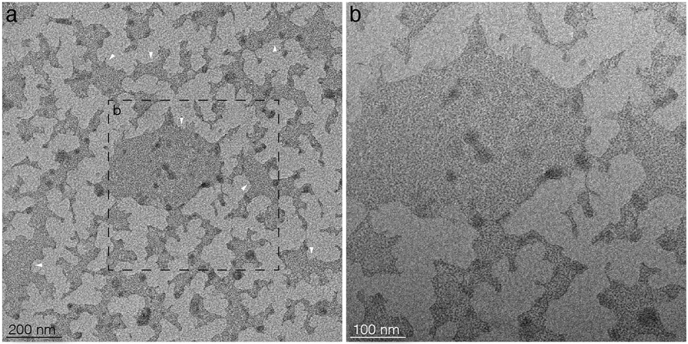
(a) Micrograph with 2D-sheets following the mixture of reconstituted proteo-liposomes with empty liposomes at a buffer contained 1x CMC detergent (DDM), at step 3 in the MEMPR method (Fig. 1, step 3). (b) Zoom-in of the dashed outlined region in (a). Similar results were obtained in all samples. White arrowheads: Open membrane-sheets after mixing reconstituted GltPh proteo-liposomes (Extended Data Fig. 2) and empty SUVs. Consistent results were obtained from > 3 reconstitution samples.
Extended Data Fig. 5. Droplet angle method for the analysis of residual detergent in the sample at different sample preparation stages.

Top left: The initial pre-physisorption mixture contains 1x CMC DDM (see main text Fig. 1, step 3). Panels 2 to 6: Buffer exchange results in ~ 1/32x CMC DDM (see main text Fig. 1, step 4). Panel 7: Inserting the sample stage into the detergent free imaging buffer in the HS-AFM fluid cell further dilutes the remaining detergent to ~ 1/1500x CMC DDM. For comparison a droplet of the detergent free buffer solution without DDM (last panel).
Extended Data Fig. 6. HS-AFM imaging of freely diffusing GltPh in extended lipid bilayers on bare mica.

(a), (b) and (c). HS-AFM frames of non-immobilized GltPh molecules in extended lipid bilayers, on the freshly cleaved mica without any pretreatment, step 5a of the MEMPR method (Fig. 1, step 5a). Freely diffusing (a) and cluster-forming (b and c) GtlPh molecules were observed in different regions of the continuous membrane (Supplementary Movies 1-3). Consistent results were obtained from > 3 HS-AFM experiments and > 3 reconstitution samples.
Extended Data Fig. 7. HS-AFM imaging of immobilized GltPh in extended lipid bilayers on poly-Lys pretreated mica.

(a), (b) and (c). HS-AFM frames of immobilized GltPh molecules in extended lipid bilayers, on the freshly cleaved mica with pretreatment of poly-Lys (coated mica), at step 5b of the MEMPR method (Fig. 1, step 5b). GltPh molecule coverage of the membrane is estimated as ~ 30% in (a), and ~ 10% in (b) and (c) (Supplementary Movies 4-6). White arrowheads: a GltPh cluster showing lateral dynamics (see main text). Consistent results were obtained from > 3 HS-AFM experiments and > 3 reconstitution samples.
Extended Data Fig. 8. Two-state conformation-time trace of a GltPh protomer showing different kinetic modes.

(a) Selected HS-AFM frames (top) and corresponding states of individual protomers (bottom) of an isolated, immobilized GltPh trimer in an extended lipid bilayer viewed from the cytoplasmic side. (b) Two-state (OFS and IFS) conformation-time trace of an individual protomer. Color coding in (a) and (b): OFS (blue) and IFS (grey). Protomer p2 switches kinetic modes: Mode 1: ~ 20 s inactive in IFS. Mode 2: ~ 40 s inactive in OFS. Mode 3: ~ 30 s highly active mode with frequent OFS-IFS transitions (Supplementary Movies 12). Two-state conformation-time traces showing different kinetic modes were observed in > 3 single molecules from different reconstitution samples.
Extended Data Fig. 9. HS-AFM fast imaging (50 frames per second) of an immobilized GltPh in extended lipid bilayers.

HS-AFM frames of an isolated and immobilized GltPh trimer in extended lipid bilayers, viewed from the cytoplasmic side on the freshly cleaved mica with pretreatment of poly-Lys (Fig. 1, step 5b). The MEMPR method enables fast imaging of single immobilized molecules with unprecedented resolutions, 0.02 s/frame and 0.25 nm/pixel, and stability, for ~ 80 s in this example (Supplementary Movies 13).
Extended Data Fig. 10. PDB Structure of a Cl− Conducting State (ClCS) GltPh.

PDB structures of GltPh IFS (XL3, gray, PDB: 6wzb), Cl− conducting state (ClCS, marron, PDB: 6wyk), IFS closed (green, PDB: 4p19, see Extended Data Fig. 1), and IFS open (green, PDB: 6x12, see Extended Data Fig. 1). Top: Superimposed structures of IFS XL3 and ClCS (left), and of IFS open and IFS closed (right). Middle: Superimposed structures of IFS open and ClCS (left), and of IFS closed and IFS XL3 (right). Bottom: Superimposed structures of IFS closed and ClCS (left), and of IFS open and IFS XL3 (right). These comparisons structurally relate ClCS to IFS open and IFS XL3 to IFS closed. IFS closed and IFS XL3 structures were collected in the apo condition. IFS open structure was collected in the presence of DL-threo-β-benzyloxyaspartate (TBOA), and ClCS in the presence of Na+ and Asp (transport condition).
Supplementary Material
Supplementary Video 1 HS-AFM movie of freely diffusing GltPh in extended lipid bilayers on freshly cleaved mica. HS-AFM movie of diffusing GltPh trimers in extended lipid bilayers, on a freshly cleaved mica, at step 5a of the MEMPR method (Fig. 1, step 5a, Extended Data Fig. 6a). Imaging parameters: 2 frame/s, 1 nm/pixel.
Supplementary Video 3 HS-AFM movie of cluster-forming GltPh in extended lipid bilayers on freshly cleaved mica area 2. HS-AFM movie of cluster-forming GltPh molecules in extended lipid bilayers, on a freshly cleaved mica, at step 5a of the MEMPR method (Fig. 1, step 5a, Extended Data Fig. 6c). Imaging parameters: 2 frame/s, 1 nm/pixel.
Supplementary Video 2 HS-AFM movie of cluster-forming GltPh in extended lipid bilayers on freshly cleaved mica area 1. HS-AFM movie of cluster-forming GltPh molecules in extended lipid bilayers, on a freshly cleaved mica, at step 5a of the MEMPR method (Fig. 1, step 5a, Extended Data Fig. 6b). Imaging parameters: 2 frame/s, 1 nm/pixel.
Supplementary Video 5 HS-AFM movie of immobilized GltPh in extended lipid bilayers on poly-Lys pretreated mica area 2. HS-AFM movie of immobilized GltPh molecules in extended lipid bilayers, on the freshly cleaved mica with pretreatment of poly-Lys (coated mica), at step 5b of the MEMPR method (Fig. 1, step 5b, Extended Data Fig. 7b). Imaging parameters: 2 frame/s, 1 nm/pixel.
Supplementary Video 4 HS-AFM movie of immobilized GltPh in extended lipid bilayers on poly-Lys pretreated mica area 1. HS-AFM movie of immobilized GltPh molecules in extended lipid bilayers, on the freshly cleaved mica with pretreatment of poly-Lys (coated mica), at step 5b of the MEMPR method (Fig. 1, step 5b, Fig. 2b, Extended Data Fig. 7a). Imaging parameters: 2 frame/s, 1 nm/pixel.
Supplementary Video 6 HS-AFM movie of immobilized GltPh in extended lipid bilayers on poly-Lys pretreated mica area 2. HS-AFM movie of immobilized GltPh molecules in extended lipid bilayers, on the freshly cleaved mica with pretreatment of poly-Lys (coated mica), at step 5b of the MEMPR method (Fig. 1, step 5b, Extended Data Fig. 7c). Imaging parameters: 2 frame/s, 1 nm/pixel.
Supplementary Video 8 HS-AFM movie of an individual GltPh trimer viewed from the extracellular side 2. HS-AFM movie of an immobilized GltPh molecule viewed from the extracellular side in an extended lipid bilayer, on the freshly cleaved mica with pretreatment of poly-Lys (coated mica), at step 5b of the MEMPR method (Fig. 1, step 5b, Fig. 2d). Imaging parameters: 10 frame/s, 0.25 nm/pixel.
Supplementary Video 7 HS-AFM movie of an individual GltPh trimer viewed from the extracellular side 1. HS-AFM movie of an immobilized GltPh molecule viewed from the extracellular side in an extended lipid bilayer, on the freshly cleaved mica with pretreatment of poly-Lys (coated mica), at step 5b of the MEMPR method (Fig. 1, step 5b, Fig. 2c). Imaging parameters: 10 frame/s, 0.25 nm/pixel.
Supplementary Video 9 HS-AFM movie of an individual GltPh trimer viewed from the cytoplasmic side 1. HS-AFM movie of an immobilized GltPh molecule viewed from the extracellular side in an extended lipid bilayer, on the freshly cleaved mica with pretreatment of poly-Lys (coated mica), at step 5b of the MEMPR method (Fig. 1, step 5b, Fig. 2e). Imaging parameters: 10 frame/s, 0.25 nm/pixel.
Supplementary Video 10 HS-AFM movie of an individual GltPh trimer viewed from the cytoplasmic side 2. HS-AFM movie of an immobilized GltPh molecule viewed from the extracellular side in an extended lipid bilayer, on the freshly cleaved mica with pretreatment of poly-Lys (coated mica), at step 5b of the MEMPR method (Fig. 1, step 5b, Fig. 2f). Imaging parameters: 10 frame/s, 0.25 nm/pixel.
Supplementary Video 12 HS-AFM movie of a GltPh protomer showing different kinetic modes. HS-AFM movie of an immobilized GltPh trimer viewed from the cytoplasmic side in an extended lipid bilayer, on the freshly cleaved mica with pretreatment of poly-Lys (coated mica), at step 5b of the MEMPR method (Fig. 1, step 5b, Extended Data Fig. 8). One protomer displayed switching modes: Mode 1: ~ 20 s inactive in IFS. Mode 2: ~ 40 s inactive in OFS. Mode 3: ~ 30 s highly active mode with frequent OFS-IFS transitions. Imaging parameters: 10 frame/s, 0.25 nm/pixel.
Supplementary Video 11 HS-AFM movie of a dimer of GltPh trimers. HS-AFM movie of a dimer of GltPh trimer viewed from the extracellular side in an extended lipid bilayer, on the freshly cleaved mica with pretreatment of poly-Lys (coated mica), at step 5b of the MEMPR method (Fig. 1, step 5b, Fig. 2g). Imaging parameters: 10 frame/s, 0.5 nm/pixel.
Supplementary Video 13 HS-AFM fast imaging of an individual GltPh trimer. HS-AFM movie of an immobilized GltPh trimer viewed from the cytoplasmic side in an extended lipid bilayer, on the freshly cleaved mica with pretreatment of poly-Lys (coated mica), at step 5b of the MEMPR method (Fig. 1, step 5b, Extended Data Fig. 9). The MEMPR method enables fast imaging of single immobilized molecules with resolutions of 0.02 s/frame and 0.25 nm/s, and stability, for ~ 80 s in this example.
Acknowledgments
General: The authors thank Jeremy S Dittman for important discussions. The authors thank Motonori Imamura, Yangang Pan, and Eunji Shin for the application of MEMPR to different membrane protein-lipid systems.
Funding: This work was funded by grants from the National Institute of Health (NIH), National Center for Complementary and Integrative Health (NCCIH), DP1AT010874 [Scheuring] and National Institute of Neurological Disorders and Stroke (NINDS), R01NS110790 [Scheuring].
Footnotes
Competing Interests Statement
The authors declare that they have no competing interests.
Data availability
All data supporting the findings of this manuscript are available within the article, supplementary information files, and source data file, provided with this paper. Additional information and raw data are available from the corresponding author upon reasonable request. PDB structures used in this article are available in the protein data bank (PDB) with the following access codes: 6X17, 6X12, 4OYE, 4P19, 6WZB, and 6WYK. The reporting summary for this article is available as a supplementary information file.
Code availability
Codes used for HS-AFM single-molecule structural analysis and LAFM map construction are available on Github (https://github.com/rafaeljiang23/SingleMoleculeStructrualBiology).
References
- 1.Tzingounis AV & Wadiche JI Glutamate transporters: confining runaway excitation by shaping synaptic transmission. Nat Rev Neurosci 8, 935–947 (2007). 10.1038/nrn2274 [DOI] [PubMed] [Google Scholar]
- 2.Danbolt NC Glutamate uptake. Prog Neurobiol 65, 1–105 (2001). 10.1016/s0301-0082(00)00067-8 [DOI] [PubMed] [Google Scholar]
- 3.Yernool D, Boudker O, Jin Y & Gouaux E Structure of a glutamate transporter homologue from Pyrococcus horikoshii. Nature 431, 811–818 (2004). 10.1038/nature03018 [DOI] [PubMed] [Google Scholar]
- 4.Wang X & Boudker O Large domain movements through the lipid bilayer mediate substrate release and inhibition of glutamate transporters. Elife 9 (2020). 10.7554/eLife.58417 [DOI] [PMC free article] [PubMed] [Google Scholar]
- 5.Verdon G & Boudker O Crystal structure of an asymmetric trimer of a bacterial glutamate transporter homolog. Nat Struct Mol Biol 19, 355–357 (2012). 10.1038/nsmb.2233 [DOI] [PMC free article] [PubMed] [Google Scholar]
- 6.Reyes N, Ginter C & Boudker O Transport mechanism of a bacterial homologue of glutamate transporters. Nature 462, 880–885 (2009). 10.1038/nature08616 [DOI] [PMC free article] [PubMed] [Google Scholar]
- 7.Reyes N, Oh S & Boudker O Binding thermodynamics of a glutamate transporter homolog. Nat Struct Mol Biol 20, 634–640 (2013). 10.1038/nsmb.2548 [DOI] [PMC free article] [PubMed] [Google Scholar]
- 8.Verdon G, Oh S, Serio RN & Boudker O Coupled ion binding and structural transitions along the transport cycle of glutamate transporters. Elife 3, e02283 (2014). 10.7554/eLife.02283 [DOI] [PMC free article] [PubMed] [Google Scholar]
- 9.Arkhipova V. et al. Binding and transport of D-aspartate by the glutamate transporter homolog Glt. Elife 8 (2019). 10.7554/eLife.45286 [DOI] [PMC free article] [PubMed] [Google Scholar]
- 10.Garaeva AA, Guskov A, Slotboom DJ & Paulino C A one-gate elevator mechanism for the human neutral amino acid transporter ASCT2. Nat Commun 10, 3427 (2019). 10.1038/s41467-019-11363-x [DOI] [PMC free article] [PubMed] [Google Scholar]
- 11.Arkhipova V, Guskov A & Slotboom DJ Structural ensemble of a glutamate transporter homologue in lipid nanodisc environment. Nat Commun 11, 998 (2020). 10.1038/s41467-020-14834-8 [DOI] [PMC free article] [PubMed] [Google Scholar]
- 12.Guskov A, Jensen S, Faustino I, Marrink SJ & Slotboom DJ Coupled binding mechanism of three sodium ions and aspartate in the glutamate transporter homologue Glt. Nat Commun 7, 13420 (2016). 10.1038/ncomms13420 [DOI] [PMC free article] [PubMed] [Google Scholar]
- 13.Alleva C. et al. Na + -dependent gate dynamics and electrostatic attraction ensure substrate coupling in glutamate transporters. Sci Adv 6 (2020). 10.1126/sciadv.aba9854 [DOI] [PMC free article] [PubMed] [Google Scholar]
- 14.Chen I. et al. Glutamate transporters have a chloride channel with two hydrophobic gates. Nature 591, 327–331 (2021). 10.1038/s41586-021-03240-9 [DOI] [PMC free article] [PubMed] [Google Scholar]
- 15.Groeneveld M & Slotboom DJ Na(+):aspartate coupling stoichiometry in the glutamate transporter homologue Glt(Ph). Biochemistry 49, 3511–3513 (2010). 10.1021/bi100430s [DOI] [PubMed] [Google Scholar]
- 16.Zerangue N & Kavanaugh MP Flux coupling in a neuronal glutamate transporter. Nature 383, 634–637 (1996). 10.1038/383634a0 [DOI] [PubMed] [Google Scholar]
- 17.Ando T. et al. A high-speed atomic force microscope for studying biological macromolecules. Proc Natl Acad Sci U S A 98, 12468–12472 (2001). 10.1073/pnas.211400898 [DOI] [PMC free article] [PubMed] [Google Scholar]
- 18.Ando T, Uchihashi T & Scheuring S Filming biomolecular processes by high-speed atomic force microscopy. Chem Rev 114, 3120–3188 (2014). 10.1021/cr4003837 [DOI] [PMC free article] [PubMed] [Google Scholar]
- 19.Akyuz N. et al. Transport domain unlocking sets the uptake rate of an aspartate transporter. Nature 518, 68–73 (2015). 10.1038/nature14158 [DOI] [PMC free article] [PubMed] [Google Scholar]
- 20.Akyuz N, Altman RB, Blanchard SC & Boudker O Transport dynamics in a glutamate transporter homologue. Nature 502, 114–118 (2013). 10.1038/nature12265 [DOI] [PMC free article] [PubMed] [Google Scholar]
- 21.Erkens GB, Hänelt I, Goudsmits JM, Slotboom DJ & van Oijen AM Unsynchronised subunit motion in single trimeric sodium-coupled aspartate transporters. Nature 502, 119–123 (2013). 10.1038/nature12538 [DOI] [PubMed] [Google Scholar]
- 22.Huysmans GHM, Ciftci D, Wang X, Blanchard SC & Boudker O The high-energy transition state of the glutamate transporter homologue GltPh. EMBO J 40, e105415 (2021). 10.15252/embj.2020105415 [DOI] [PMC free article] [PubMed] [Google Scholar]
- 23.Ciftci D. et al. Single-molecule transport kinetics of a glutamate transporter homolog shows static disorder. Sci Adv 6, eaaz1949 (2020). 10.1126/sciadv.aaz1949 [DOI] [PMC free article] [PubMed] [Google Scholar]
- 24.Silberberg SD, Lagrutta A, Adelman JP & Magleby KL Wanderlust kinetics and variable Ca(2+)-sensitivity of dSlo [correction of Drosophila], a large conductance CA(2+)-activated K+ channel, expressed in oocytes. Biophys J 71, 2640–2651 (1996). [PMC free article] [PubMed] [Google Scholar]
- 25.Poon K, Nowak LM & Oswald RE Characterizing single-channel behavior of GluA3 receptors. Biophys J 99, 1437–1446 (2010). 10.1016/j.bpj.2010.06.058 [DOI] [PMC free article] [PubMed] [Google Scholar]
- 26.Hirschberg B, Maylie J, Adelman JP & Marrion NV Gating of recombinant small-conductance Ca-activated K+ channels by calcium. J Gen Physiol 111, 565–581 (1998). 10.1085/jgp.111.4.565 [DOI] [PMC free article] [PubMed] [Google Scholar]
- 27.Milone M. et al. Mode switching kinetics produced by a naturally occurring mutation in the cytoplasmic loop of the human acetylcholine receptor epsilon subunit. Neuron 20, 575–588 (1998). 10.1016/s0896-6273(00)80996-4 [DOI] [PubMed] [Google Scholar]
- 28.Rothberg BS & Magleby KL Kinetic structure of large-conductance Ca2+-activated K+ channels suggests that the gating includes transitions through intermediate or secondary states. A mechanism for flickers. J Gen Physiol 111, 751–780 (1998). 10.1085/jgp.111.6.751 [DOI] [PMC free article] [PubMed] [Google Scholar]
- 29.Kosmidis E. et al. Regulation of the mammalian-brain V-ATPase through ultraslow mode-switching. Nature 611, 827–834 (2022). 10.1038/s41586-022-05472-9 [DOI] [PMC free article] [PubMed] [Google Scholar]
- 30.Ruan Y. et al. Direct visualization of glutamate transporter elevator mechanism by high-speed AFM. Proc Natl Acad Sci U S A 114, 1584–1588 (2017). 10.1073/pnas.1616413114 [DOI] [PMC free article] [PubMed] [Google Scholar]
- 31.Matin TR, Heath GR, Huysmans GHM, Boudker O & Scheuring S Millisecond dynamics of an unlabeled amino acid transporter. Nat Commun 11, 5016 (2020). 10.1038/s41467-020-18811-z [DOI] [PMC free article] [PubMed] [Google Scholar]
- 32.Heath GR & Scheuring S Advances in high-speed atomic force microscopy (HS-AFM) reveal dynamics of transmembrane channels and transporters. Curr Opin Struct Biol 57, 93–102 (2019). 10.1016/j.sbi.2019.02.008 [DOI] [PMC free article] [PubMed] [Google Scholar]
- 33.Jiang Y. et al. Membrane-mediated protein interactions drive membrane protein organization. Nat Commun 13, 7373 (2022). 10.1038/s41467-022-35202-8 [DOI] [PMC free article] [PubMed] [Google Scholar]
- 34.Phillips R, Ursell T, Wiggins P & Sens P Emerging roles for lipids in shaping membrane-protein function. Nature 459, 379–385 (2009). 10.1038/nature08147 [DOI] [PMC free article] [PubMed] [Google Scholar]
- 35.Gao J, Hou R, Li L & Hu J Membrane-Mediated Interactions Between Protein Inclusions. Front Mol Biosci 8, 811711 (2021). 10.3389/fmolb.2021.811711 [DOI] [PMC free article] [PubMed] [Google Scholar]
- 36.Eddy SR Hidden Markov models. Curr Opin Struct Biol 6, 361–365 (1996). 10.1016/s0959-440x(96)80056-x [DOI] [PubMed] [Google Scholar]
- 37.Eddy SR What is a hidden Markov model? Nat Biotechnol 22, 1315–1316 (2004). 10.1038/nbt1004-1315 [DOI] [PubMed] [Google Scholar]
- 38.Zhou J & Sutherland ML Glutamate transporter cluster formation in astrocytic processes regulates glutamate uptake activity. J Neurosci 24, 6301–6306 (2004). 10.1523/JNEUROSCI.1404-04.2004 [DOI] [PMC free article] [PubMed] [Google Scholar]
- 39.Nakagawa T, Otsubo Y, Yatani Y, Shirakawa H & Kaneko S Mechanisms of substrate transport-induced clustering of a glial glutamate transporter GLT-1 in astroglial-neuronal cultures. Eur J Neurosci 28, 1719–1730 (2008). 10.1111/j.1460-9568.2008.06494.x [DOI] [PubMed] [Google Scholar]
- 40.Heath GR et al. Layer-by-Layer Assembly of Supported Lipid Bilayer Poly-L-Lysine Multilayers. Biomacromolecules 17, 324–335 (2016). 10.1021/acs.biomac.5b01434 [DOI] [PubMed] [Google Scholar]
- 41.Heath GR et al. Localization atomic force microscopy. Nature 594, 385–390 (2021). 10.1038/s41586-021-03551-x [DOI] [PMC free article] [PubMed] [Google Scholar]
- 42.E BR Dynamic Programming. (Princeton University Press, 2010). [Google Scholar]
- 43.Jolliffe IT & Cadima J Principal component analysis: a review and recent developments. Philos Trans A Math Phys Eng Sci 374, 20150202 (2016). 10.1098/rsta.2015.0202 [DOI] [PMC free article] [PubMed] [Google Scholar]
- 44.Hidden Markov Modeling in Single-Molecule Biophysics , bookTitle= Encyclopedia of Biophysics. (Springer Berlin Heidelberg, 2013). [Google Scholar]
- 45.Krogh A, Brown M, Mian IS, Sjölander K & Haussler D Hidden Markov models in computational biology. Applications to protein modeling. J Mol Biol 235, 1501–1531 (1994). 10.1006/jmbi.1994.1104 [DOI] [PubMed] [Google Scholar]
- 46.Sgouralis I & Pressé S An Introduction to Infinite HMMs for Single-Molecule Data Analysis. Biophys J 112, 2021–2029 (2017). 10.1016/j.bpj.2017.04.027 [DOI] [PMC free article] [PubMed] [Google Scholar]
- 47.Vijayabaskar MS Introduction to Hidden Markov Models and Its Applications in Biology. Methods Mol Biol 1552, 1–12 (2017). 10.1007/978-1-4939-6753-7_1 [DOI] [PubMed] [Google Scholar]
- 48.Baggenstoss PM A modified Baum-Welch algorithm for hidden Markov models with multiple observation spaces. IEEE Transactions on Speech and Audio Processing 9, 411–416 (2001). 10.1109/89.917686 [DOI] [Google Scholar]
- 49.Huang Y. et al. Environmentally Ultrasensitive Fluorine Probe to Resolve Protein Conformational Ensembles by. J Am Chem Soc 145, 8583–8592 (2023). 10.1021/jacs.3c01003 [DOI] [PMC free article] [PubMed] [Google Scholar]
- 50.Chen I, Wu Q, Font J & Ryan RM The twisting elevator mechanism of glutamate transporters reveals the structural basis for the dual transport-channel functions. Curr Opin Struct Biol 75, 102405 (2022). 10.1016/j.sbi.2022.102405 [DOI] [PubMed] [Google Scholar]
Methods-only References
- 51.Qiu B, Matthies D, Fortea E, Yu Z & Boudker O Cryo-EM structures of excitatory amino acid transporter 3 visualize coupled substrate, sodium, and proton binding and transport. Sci Adv 7 (2021). 10.1126/sciadv.abf5814 [DOI] [PMC free article] [PubMed] [Google Scholar]
- 52.Miyagi A & Scheuring S A novel phase-shift-based amplitude detector for a high-speed atomic force microscope. Rev Sci Instrum 89, 083704 (2018). 10.1063/1.5038095 [DOI] [PubMed] [Google Scholar]
- 53.Miyagi A & Scheuring S Automated force controller for amplitude modulation atomic force microscopy. Rev Sci Instrum 87, 053705 (2016). 10.1063/1.4950777 [DOI] [PubMed] [Google Scholar]
- 54.McLachlan GJ & David P Finite Mixture Models. (John Wiley & Sons, Inc, 2000). [Google Scholar]
- 55.Gonzalez RC, Woods RE & Eddins SL Digital Image Processing Using MATLAB. 3rd edn, (Gatesmark Publishing, 2020). [Google Scholar]
- 56.Tan Y, Li G, Duan H & Li C Enhancement of Medical Image Details via Wavelet Homomorphic Filtering Transform. Journal of Intelligent System 23, 83–94 (2014). 10.1515/jisys-2013-0061 [DOI] [Google Scholar]
Associated Data
This section collects any data citations, data availability statements, or supplementary materials included in this article.
Supplementary Materials
Supplementary Video 1 HS-AFM movie of freely diffusing GltPh in extended lipid bilayers on freshly cleaved mica. HS-AFM movie of diffusing GltPh trimers in extended lipid bilayers, on a freshly cleaved mica, at step 5a of the MEMPR method (Fig. 1, step 5a, Extended Data Fig. 6a). Imaging parameters: 2 frame/s, 1 nm/pixel.
Supplementary Video 3 HS-AFM movie of cluster-forming GltPh in extended lipid bilayers on freshly cleaved mica area 2. HS-AFM movie of cluster-forming GltPh molecules in extended lipid bilayers, on a freshly cleaved mica, at step 5a of the MEMPR method (Fig. 1, step 5a, Extended Data Fig. 6c). Imaging parameters: 2 frame/s, 1 nm/pixel.
Supplementary Video 2 HS-AFM movie of cluster-forming GltPh in extended lipid bilayers on freshly cleaved mica area 1. HS-AFM movie of cluster-forming GltPh molecules in extended lipid bilayers, on a freshly cleaved mica, at step 5a of the MEMPR method (Fig. 1, step 5a, Extended Data Fig. 6b). Imaging parameters: 2 frame/s, 1 nm/pixel.
Supplementary Video 5 HS-AFM movie of immobilized GltPh in extended lipid bilayers on poly-Lys pretreated mica area 2. HS-AFM movie of immobilized GltPh molecules in extended lipid bilayers, on the freshly cleaved mica with pretreatment of poly-Lys (coated mica), at step 5b of the MEMPR method (Fig. 1, step 5b, Extended Data Fig. 7b). Imaging parameters: 2 frame/s, 1 nm/pixel.
Supplementary Video 4 HS-AFM movie of immobilized GltPh in extended lipid bilayers on poly-Lys pretreated mica area 1. HS-AFM movie of immobilized GltPh molecules in extended lipid bilayers, on the freshly cleaved mica with pretreatment of poly-Lys (coated mica), at step 5b of the MEMPR method (Fig. 1, step 5b, Fig. 2b, Extended Data Fig. 7a). Imaging parameters: 2 frame/s, 1 nm/pixel.
Supplementary Video 6 HS-AFM movie of immobilized GltPh in extended lipid bilayers on poly-Lys pretreated mica area 2. HS-AFM movie of immobilized GltPh molecules in extended lipid bilayers, on the freshly cleaved mica with pretreatment of poly-Lys (coated mica), at step 5b of the MEMPR method (Fig. 1, step 5b, Extended Data Fig. 7c). Imaging parameters: 2 frame/s, 1 nm/pixel.
Supplementary Video 8 HS-AFM movie of an individual GltPh trimer viewed from the extracellular side 2. HS-AFM movie of an immobilized GltPh molecule viewed from the extracellular side in an extended lipid bilayer, on the freshly cleaved mica with pretreatment of poly-Lys (coated mica), at step 5b of the MEMPR method (Fig. 1, step 5b, Fig. 2d). Imaging parameters: 10 frame/s, 0.25 nm/pixel.
Supplementary Video 7 HS-AFM movie of an individual GltPh trimer viewed from the extracellular side 1. HS-AFM movie of an immobilized GltPh molecule viewed from the extracellular side in an extended lipid bilayer, on the freshly cleaved mica with pretreatment of poly-Lys (coated mica), at step 5b of the MEMPR method (Fig. 1, step 5b, Fig. 2c). Imaging parameters: 10 frame/s, 0.25 nm/pixel.
Supplementary Video 9 HS-AFM movie of an individual GltPh trimer viewed from the cytoplasmic side 1. HS-AFM movie of an immobilized GltPh molecule viewed from the extracellular side in an extended lipid bilayer, on the freshly cleaved mica with pretreatment of poly-Lys (coated mica), at step 5b of the MEMPR method (Fig. 1, step 5b, Fig. 2e). Imaging parameters: 10 frame/s, 0.25 nm/pixel.
Supplementary Video 10 HS-AFM movie of an individual GltPh trimer viewed from the cytoplasmic side 2. HS-AFM movie of an immobilized GltPh molecule viewed from the extracellular side in an extended lipid bilayer, on the freshly cleaved mica with pretreatment of poly-Lys (coated mica), at step 5b of the MEMPR method (Fig. 1, step 5b, Fig. 2f). Imaging parameters: 10 frame/s, 0.25 nm/pixel.
Supplementary Video 12 HS-AFM movie of a GltPh protomer showing different kinetic modes. HS-AFM movie of an immobilized GltPh trimer viewed from the cytoplasmic side in an extended lipid bilayer, on the freshly cleaved mica with pretreatment of poly-Lys (coated mica), at step 5b of the MEMPR method (Fig. 1, step 5b, Extended Data Fig. 8). One protomer displayed switching modes: Mode 1: ~ 20 s inactive in IFS. Mode 2: ~ 40 s inactive in OFS. Mode 3: ~ 30 s highly active mode with frequent OFS-IFS transitions. Imaging parameters: 10 frame/s, 0.25 nm/pixel.
Supplementary Video 11 HS-AFM movie of a dimer of GltPh trimers. HS-AFM movie of a dimer of GltPh trimer viewed from the extracellular side in an extended lipid bilayer, on the freshly cleaved mica with pretreatment of poly-Lys (coated mica), at step 5b of the MEMPR method (Fig. 1, step 5b, Fig. 2g). Imaging parameters: 10 frame/s, 0.5 nm/pixel.
Supplementary Video 13 HS-AFM fast imaging of an individual GltPh trimer. HS-AFM movie of an immobilized GltPh trimer viewed from the cytoplasmic side in an extended lipid bilayer, on the freshly cleaved mica with pretreatment of poly-Lys (coated mica), at step 5b of the MEMPR method (Fig. 1, step 5b, Extended Data Fig. 9). The MEMPR method enables fast imaging of single immobilized molecules with resolutions of 0.02 s/frame and 0.25 nm/s, and stability, for ~ 80 s in this example.
Data Availability Statement
All data supporting the findings of this manuscript are available within the article, supplementary information files, and source data file, provided with this paper. Additional information and raw data are available from the corresponding author upon reasonable request. PDB structures used in this article are available in the protein data bank (PDB) with the following access codes: 6X17, 6X12, 4OYE, 4P19, 6WZB, and 6WYK. The reporting summary for this article is available as a supplementary information file.
Codes used for HS-AFM single-molecule structural analysis and LAFM map construction are available on Github (https://github.com/rafaeljiang23/SingleMoleculeStructrualBiology).