DeepLoop robustly maps chromatin interactions from sparse allele-resolved or single-cell Hi-C data at kilobase resolution

Abstract

Mapping chromatin loops from noisy Hi-C heatmaps remains a major challenge. Here we present DeepLoop, which performs rigorous bias-correction followed by deep-learning-based signal-enhancement for robust chromatin interaction mapping from low-depth Hi-C data. DeepLoop enables loop-resolution single-cell Hi-C analysis. It also achieves a cross-platform convergence between different Hi-C protocols and micro-C. DeepLoop allowed us to map the genetic and epigenetic determinants of allele-specific (AS) chromatin interactions in human genome. We nominate new loci with AS-interactions governed by imprinting or allelic DNA methylation. We also discovered that in the inactivated X chromosome (Xi), local loops at the DXZ4 “megadomain” boundary escape X-inactivation, but the FIRRE “superloop” locus does not escape. Importantly, DeepLoop can pinpoint heterozygous SNPs and large structure variants (SVs) that cause allelic chromatin loops, many of which rewire enhancers with transcription consequences. Taken together, DeepLoop expands the use of Hi-C to provide loop-resolution insights into the genetics of 3D genome.

Hi-C has transformed our understanding of mammalian genome organization and can reliably identify high-order 3D genome features such as compartments and topological associated domains (TADs)^1–4. However, when resolution reaches kilobase-scale, the Hi-C contact heatmaps quickly become noisy due to the increasingly complex bias structure and severe data sparsity^5–9. To date, genome-wide mapping of chromatin loops, especially the enhancer-promoter (E-P) interactions within TADs (sub-TAD), remains a major challenge in Hi-C analyses. Consequently, scientists often turn to focused technologies, such as ChIA-PET, promoter capture Hi-C (pcHi-C), HiChIP/PLAC-seq, etc., hoping for better signal-to-noise ratios at selected loci^10–15, even though these approaches only identify a subset of all interactions

Bias and noise are two distinct types of errors in Hi-C data. Here we define biases as “unwanted pattern in a Hi-C heatmap”. This definition is goal oriented. For example, to distinguish relatively weak loop signals, the strong non-specific diagonal Hi-C signal needs to be corrected as bias. Hi-C protocols using different digestion enzymes have different bias structures determined by fragment size, distance, GC content, and the interactions between these factors^5,6, the bias structure becomes more complicated when the resolution gets higher, especially at the sub-TAD mid-range (i.e., within 1–2Mb). While several methods have been developed to model and correct known sources of Hi-C biases explicitly with joint functions, the most commonly-used strategy is to “normalize” the Hi-C matrices and correct Hi-C biases implicitly with matrix balancing algorithms^{5–7,16–18}. But both explicit and implicit strategies have drawbacks^{5,6,8,9,16,17}. To improve the rigor of Hi-C bias correction, we recently developed a HiCorr pipeline that does both explicit and implicit correction⁹. Unlike the “normalization” methods^7,17, which preserve a strong diagonal signal in the contact heatmaps, HiCorr corrects distance effects in a joint function with other biases, and outputs the obs/exp ratio heatmaps for chromatin interaction profiling. When read depth is high, HiCorr generates sharper contact heatmaps, and is more robust in identifying sub-TAD chromatin loops⁹.

Theoretically, when all biases are corrected, only data sparsity contributes to the Hi-C noises. Therefore, reducing Hi-C noises is mathematically equivalent to signal enhancement. Several recent studies have pioneered the application of deep-learning techniques to enhance Hi-C signal at compartment, TAD, and loop levels^19–23. These pipelines share a similar framework to impute high-depth contact matrices from the low-depth raw or “normalized” Hi-C data. It is however important to point out that this strategy “learns” Hi-C biases in the input matrices, which may no longer be properly corrected after enhancement. This flaw is significant for loop analysis because distance effect is a major bias for loop analysis, and other Hi-C biases are also much worse at high-resolution. To address this issue, here we developed a strategy to enhance HiCorr-corrected ratio heatmaps. The resulting DeepLoop pipeline achieved striking robustness in calling loops from low-depth Hi-C data. This study will highlight the applications of DeepLoop to single-cell and allele-resolved Hi-C data analyses; both scenarios suffer from the challenge of severe data sparsity.

Results

LoopDenoise improves the robustness of Hi-C loop mapping

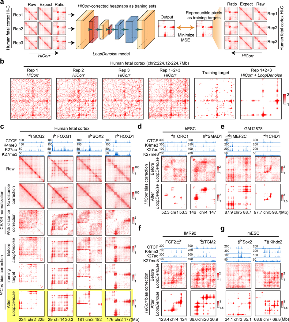
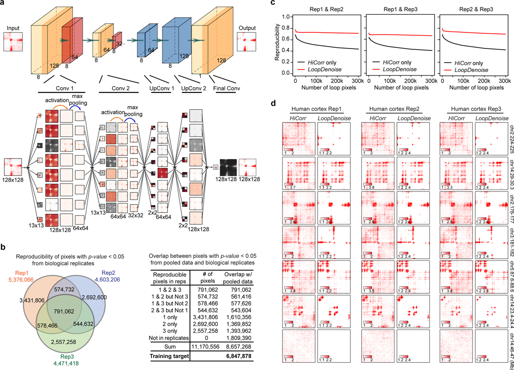
We begin with denoising high-depth Hi-C heatmaps with a 5-layer autoencoder (Figure 1a, Extended Data Figure 1a). We picked three replicates of Hi-C data in human fetal cerebral cortex²⁴ for model training; each replicate has 140~150 million mid-range (< 2Mb) cis contacts. (In this paper we use the number of mid-range cis contacts to measure “read depth”, or the total amount of data for a Hi-C experiment.) We applied HiCorr to each replicate and extracted ~18,000 submatrices at fragment resolution (~5kb) as training sets (Figure 1a–Figure 1b). As previously reported, HiCorr generates sharper distance-corrected ratio heatmaps than ICE/KR⁹ (compare row 3 and 4 in Figure 1c), but noise pixels are still present. When pooling the reads from all three replicates together, the HiCorr heatmaps are only slightly cleaner (Figure 1b). Since true loop pixels are more reproducible than noise pixels between biological replicates, we setup “training target” heatmaps by only keeping the reproducible loop pixels (Figure 1b, Extended Data Figure 1b, Methods).

Figure 1. HiCorr and LoopDenoise reveal chromatin loops from noisy Hi-C datasets.

a, Scheme showing the LoopDenoise model architecture and training. The three HiCorr-corrected human fetal brain datasets are used as training sets. The training targets are the reproducible pixels in the heatmaps from the pooled data. b, The example heatmaps from human fetal cortex Hi-C data, including three HiCorr-corrected replicates, pooled data, training target and output from LoopDenoise. c, LoopDenoise performance in the training human fetal cortex Hi-C data at 4 loci. Heatmaps of raw and various processed data are compared. Highlighted row is LoopDenoise output. d-g, Heatmaps showing the application of LoopDenoise to four independent Hi-C datasets in hESCs, GM12878, IMR90, and mESCs. The ChIP-seq tracks show raw reads pileup. See Methods for information how to determine the color scale of each heatmap.

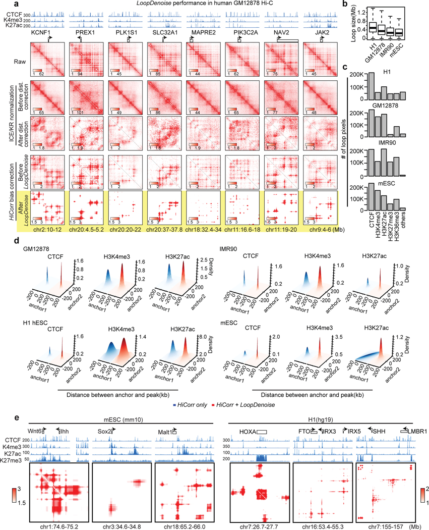
LoopDenoise removes all visible noise pixels from the HiCorr-corrected ratio heatmaps (Figure 1c, compare row 4 and 6). The denoised heatmaps are cleaner than the “training targets” (Figure 1b, and Figure 1c, compare row 5 and 6). When applied to biological replicates, LoopDenoise improves the pairwise reproducibility to 70~80% at pixel level (Extended Data Figure 1c–d). When applied to independent Hi-C datasets in hESC, IMR90, GM12878 and mESC cells^{1,6,7,9,25–27} (Supplementary Table 1), the benefits of LoopDenoise are also obvious (Figure 1d–Figure 1g, Extended Data Figure 2a). The loop pixels are better concentrated near CTCF, H3K4me3, and H3K27ac peaks after denoising^1,28–31 (Extended Data Figure 2b–d). LoopDenoise successfully reveals loop interactions at loci with well-established long-range gene regulation, such as Sox2, Wnt6, Malt1 in mESCs, and HOXA’s, FTO, SHH in hESCs (Extended Data Figure 2e)^32–35.

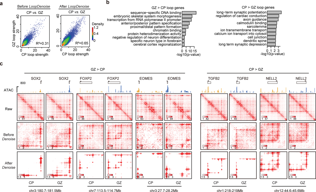
To test if the improved reproducibility will facilitate the identification of dynamic chromatin loops, we compared human cortex Hi-C data from germinal zone (GZ) and cortical plate (CP), which are two layers of developing cortex enriched with neuron progenitors and post-mitotic neurons^24,36. Indeed, the R-square between GZ and CP improves from 0.31 to 0.65 after denoising (Extended Data Figure 3a). When picking the genes associated with top 3,000 GZ- or CP-specific loop pixels, we found that the GZ loop genes are enriched with terms related to neural development, and CP loop genes are enriched with neuronal function terms (Extended Data Figure 3b). After denoising, the dynamic loop pixels are clearly recognizable at the GZ-specific (such as SOX2, FOXP2, and EOMES) and CP-specific (such as TGFB2 and NELL2) genes agreeing with GZ- or CP-specific ATAC-seq peaks³⁷ (Extended Data Figure 3c).

LoopEnhance reliably maps Hi-C loops from low-depth data

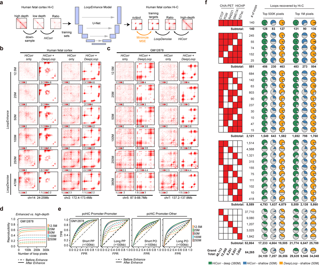
We then develop method to analyze low-depth Hi-C data. We trained a series of U-Net³⁸ LoopEnhance models using down-sampled cortex Hi-C data with 10~250M mid-range cis-contacts. Notably, we used the LoopDenoise outputs from the high-depth data as training targets which should be better representations of the “ground truth” (Figure 2a, Supplementary Figure 1a). Strikingly, although the loop signals are hardly recognizable when read depth is below 50Mb, the enhanced heatmaps from low-depth Hi-C data are nearly identical (Figure 2b). LoopEnhance models created with cortex data also perform very well in the independent GM12878 datasets (Figure 2c). When comparing the enhanced heatmaps to the full data (~380M mid-range cis contacts), we found no compromise of performance (pixel-level reproducibility > 70%) when the read depth is lowered to 100M; the pixel level reproducibility remains above 50% even when the sequencing depth is lower to 12.5M (Figure 2d). We also trained new DeepLoop models (LoopDenoise and LoopEnhance) with Hi-C data from H9 hESCs and confirmed that the choice of training sets does not affect the results (Supplementary Figure 1b–c). Because the pixel intensity in DeepLoop heatmaps represents Hi-C signal enrichment, we can directly call top loop pixels as interactions. Note that DeepLoop does not output an explicit list of discrete “loops”; converting “loop pixels” to “loops” requires new algorithms and parameters, which will inevitably introduce new biases. Therefore, we keep DeepLoop as a “What-You-See-Is-What-You-Get” method.

Figure 2. LoopEnhance enables sensitive and robust loop calling from low-depth Hi-C data.

a, Scheme showing the architecture and training of LoopEnhance model. Left: Down-sampling from high-depth human fetal cortex Hi-C data as training sets after HiCorr-correction. Middle: the U-Net architecture of LoopEnhance. Right: Training targets are high-depth human fetal brain data after both HiCorr and LoopDenoise. b, Heatmap examples showing the outputs of LoopEnhance when applied to down-sampled human fetal cortex data (training sets) at variable depths. Two loci are shown. The last row is LoopDenoise output using the full dataset (training target). c, Heatmap examples showing the application of LoopEnhance to down-sampled independent GM12878 data. The full GM12878 data were analyzed with LoopDenoise (last row). In both b and c, sequencing depth on the left indicate the numbers of mid-range (<2Mb) cis contacts. d, Reproducibility, the fraction of overlapped loop pixels, between down-sampled and full-depth GM12878 data when the same numbers of loop pixels are called. For comparison, LoopDenoise was used on the full-depth GM12878 data. Solid lines: HiCorr and LoopEnhance are applied to down-sampled data; dash lines: Only HiCorr are applied. e, ROC curves showing the recovery of GM12878 pcHi-C loops with enhanced low-depth Hi-C data. The significant (p-value<0.01, three-parameter Weibull distribution) pcHi-C interactions (PP and PO) in GM12878 are considered as true positives. Solid lines: HiCorr + LoopDenoise; dashed lines: HiCorr only. f, The loops identified from five published ChIA-PET and HiChIP studies in GM12878 are grouped by their recurrence among these experiments. The loop number and subtotal for each “recurrence” group were listed. Pie charts indicate the percentage of each group of loops recovered by Hi-C map when calling top 500K or 1M loop pixels. Green: 380M-depth HiCorr map; blue: 50M-depth HiCorr map; orange: 50M-depth DeepLoop-enhanced map.

We next compared the DeepLoop pixels in GM12878 cells to the ~83K loops called by pcHi-C in the same cell line³⁹. We classified the pcHi-C loops into promoter-promoter interactions (PP, the fragments of both ends were captured with promoter probes) and promoter-other interactions (PO, only one end of the interaction was captured), and further divided these loops into long-range (>100kb) and short-range (<100kb) categories. DeepLoop improves the ROC curves in all categories especially the long-range ones (Figure 2e); this is consistent with DeepLoop’s noise reduction function, since Hi-C matrices are noisier at long range due to more severe data sparsity.

We also collected 5 sets of ChIA-PET or HiChIP data in GM12878 cells done with CTCF, PolII, RAD21, SMC1A and H3K27ac antibodies^14,40–43. The numbers of loops from these datasets are highly variable (3.6K to 48K)), with a grand total ~64K (Figure 2f). Clearly, each experiment only captures a subset of all interactions. We classified all loops based on their recurrence among these experiments and examined how well Hi-C recovers each category. With DeepLoop, a downsampled 50M-depth Hi-C map can recover 7,051 (62%) and 8,260 (72%) of the 11,401 “recurrent” (in least two experiments) loops when calling 500K and 1M top loop pixels, in contrast to only 23% and 29% before enhancement. The recovery of the ~53K “non-recurrent” loops improves even more. In fact, the enhanced 50M-map outperforms the un-enhanced 380M full-data map in all loop categories (Figure 2f). Notably, the cost to generate 50M-depth Hi-C data is already lower than one ChIA-PET or HiChIP experiment.

DeepLoop Hi-C maps converge with micro-C maps

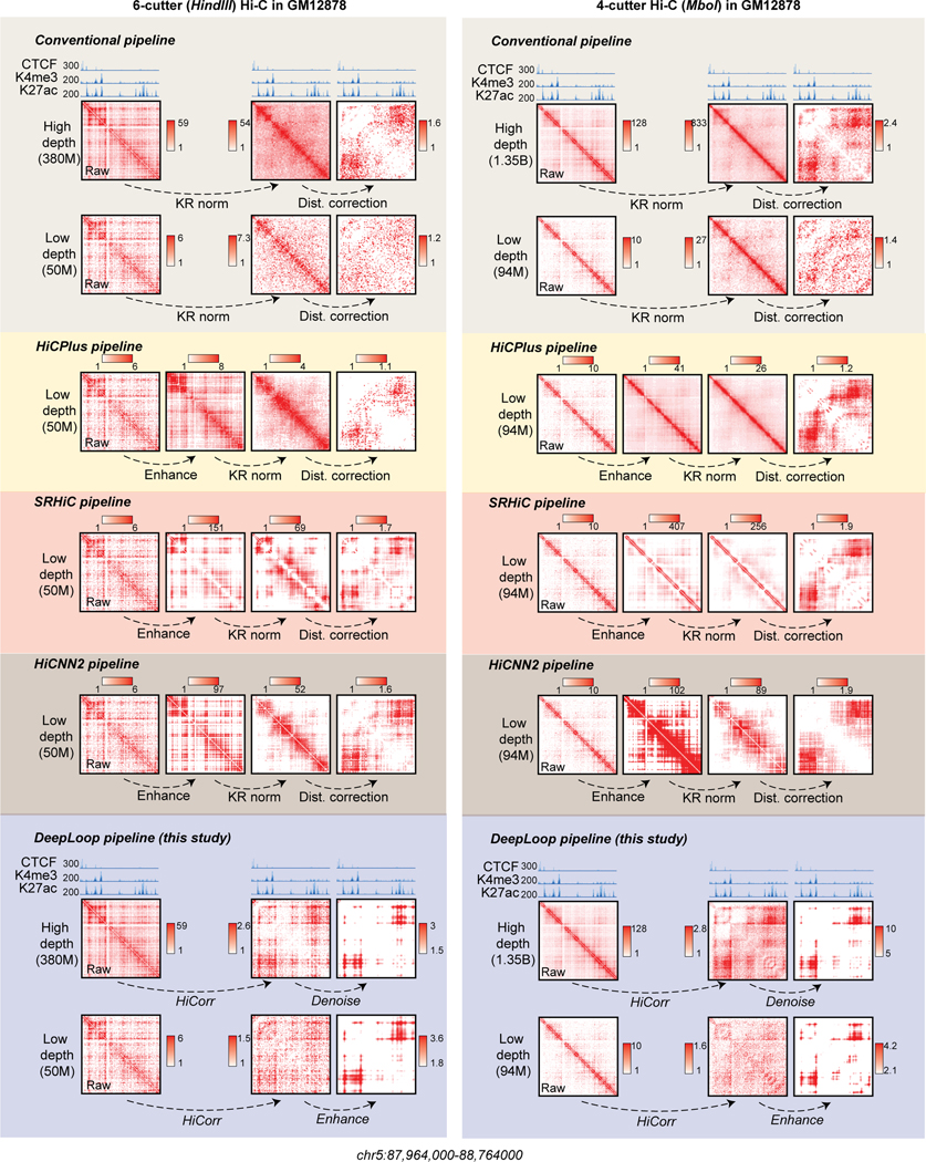
Although DeepLoop is trained with 6-cutter Hi-C data, since its bias-correction is independent from the noise-reduction module, we only need to adjust HiCorr for DeepLoop to work for other Hi-C-like data. Indeed, both LoopDenoise and LoopEnhance work very well on the MboI-based GM12878 in situ Hi-C data⁷ (examples in Extended Data Figure 4). Interestingly, although with conventional pipeline, 4-cutter Hi-C heatmaps are sharper than 6-cutter Hi-C heatmaps, DeepLoop heatmaps are very similar, indicating that HiCorr better removes platform-specific biases and supports cross-platform comparison. For the same reason, DeepLoop substantially outperforms other Hi-C enhancing pipelines including HiCPlus²¹, HiCNN2⁴⁴, and SRHiC²³ (Extended Data Figure 4).

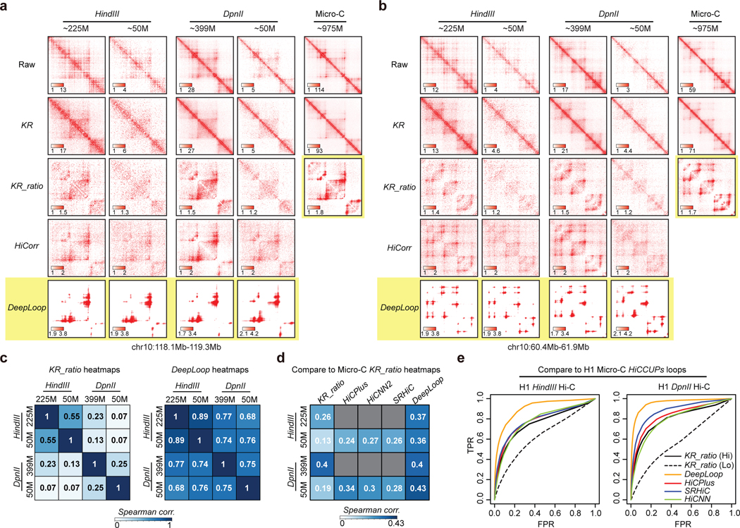
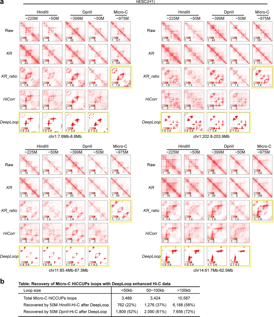
To further explore the cross-platform consistency, we compare the published ultradeep Hi-C data in H1 hESCs prepared with HindIII, DpnII, and micrococcal nuclease (Micro-C)^9,27,45,46. As expected⁴⁷, for raw, KR, and KR-ratio heatmaps, Micro-C is sharper than both HindIII- and DpnII-Hi-C; DpnII-Hi-C is shaper than HindIII-Hi-C (examples in Figure 3a,b and Extended Data Figure 5a). However, DeepLoop heatmaps from HindIII and DpnII Hi-C are much more similar at pixel level, regardless of the read-depth (Figure 3c). Importantly, when digestion resolution gets higher (from Hi-C to micro-C), the KR-ratio heatmaps become sharper and more similar to DeepLoop outputs (Figure 3a,b and Extended Data Figure 5a). When we compare other signal enhancement methods using micro-C KR-ratio heatmaps as reference, DeepLoop shows highest correlation coefficient (Figure 3d). Finally, we call 17.5K micro-C loops at 5kb resolution using standard KR-HICCUPS pipeline, then perform ROC analyses using these loops as true positives. DeepLoop-enhanced low-depth (50M) Hi-C data performs better than all other pipelines, even better than the KR-processed full-depth data (Figure 3e).

Figure 3. DeepLoop outputs convergent Hi-C loop profiles regardless of the read depth and digestion resolution.

a-b, Heatmap examples showing the outputs of different pipelines with full depth or down-sampled (50M) HindIII- or DpnII-based Hi-C data in H1 hESCs. The last column shows the KR-processed heatmaps from ultradeep Micro-C data. c, left: the Spearman correlations between Hi-C experiments with different restriction enzymes and read depths when KR-ratio contact heatmaps are compared at pixel level. Right: same as left but DeepLoop outputs were used in the comparison. d, the spearman correlations between Micro-C KR-ratio heatmaps and the outputs of various pipelines with HindIII- or DpnII-based Hi-C data. e, ROC curves comparing the performance of different enhancing pipelines in recovering the micro-C loops when applied to HindIII- or DpnII-base H1 hESC Hi-C data. For all Hi-C analysis pipelines, loop pixels are called from the ratio heatmaps after ranked by intensity. Pixels in Micro-C HICCUPS loops (after KR-normalization) are treated as true positives. KR-ratio heatmaps from full-depth (solid black curve) or down-sampled Hi-C (dashed black curve) are plotted as reference.

Micro-C is expected to reveal more small loops (<50kb) than 6-cutter or 4-cutter Hi-C with standard HICCUPS pipeline^45,47,48. We found that with 4-cutter Hi-C, DeepLoop recovers most of the micro-C small loops and the recovery rate is only slightly lower than large loops (Extended Data Figure 5b). However, DeepLoop-enhanced 6-cutter Hi-C misses most small micro-C loops. This indicates that HindIII hits a hard limit for small loop detection due to big fragment size: enough restriction sites need to be cut between the two anchors to discern a small loop. Notably, micro-C may find even smaller loops at higher resolution^45,48. Improving DeepLoop resolution will be an interesting future direction. Regardless, DeepLoop achieves better cross-platform convergence between Hi-C and Micro-C.

Apply DeepLoop to sparse and single cell Hi-C data

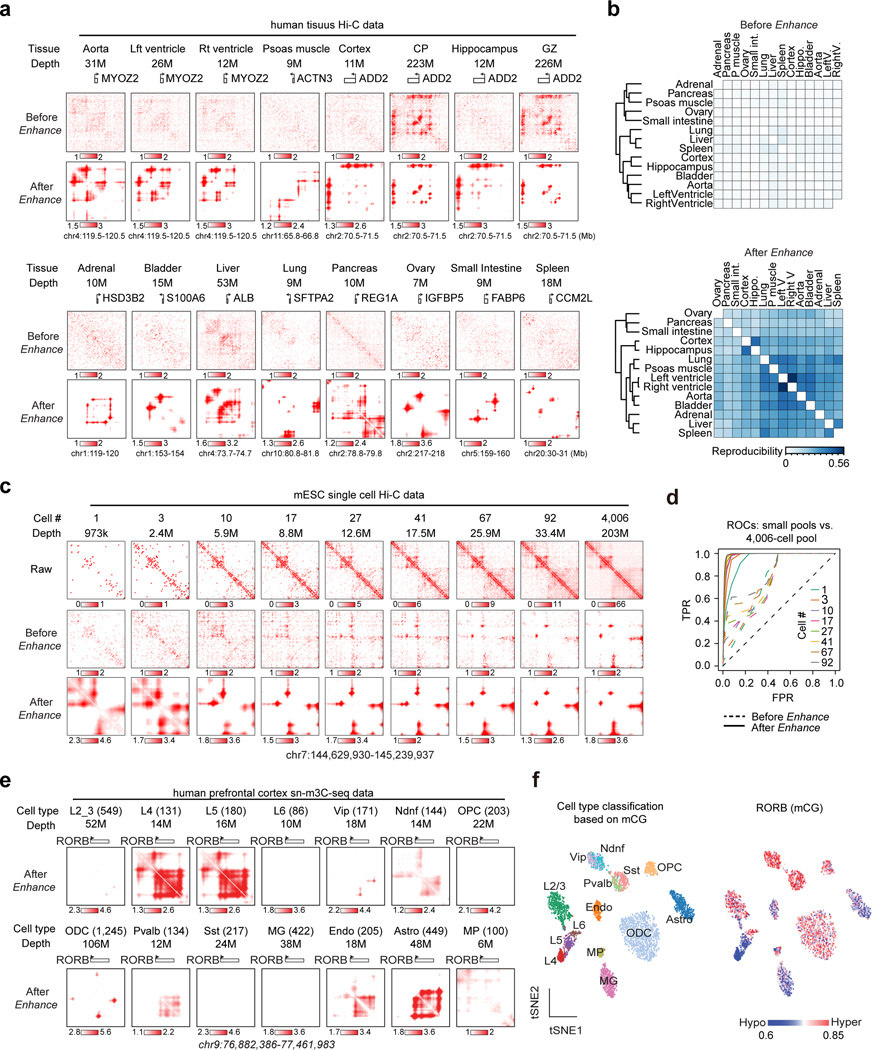
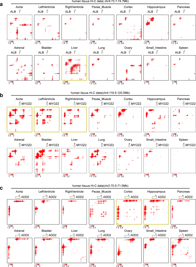
We firstly enhanced published sparse Hi-C data in 14 human tissues (depth 7~53M mid-range cis contacts)^29,30,49. We observed specific loop interactions near many tissue-marker genes after enhancement, such as ALB (liver), MYOZ2 (aorta, left and right ventricle), and ADD2 (cortex, hippocampus, CP and GZ) (Figure 4a, Extended Data Figure 6). Quantitively, the pixel-level correlation between related tissues improved tremendously after enhancement (Figure 4b).

Figure 4. DeepLoop identifies chromatin interactions from low-depth and single cell Hi-C data.

a, Contact heatmaps of exemplary marker genes in 14 published low-depth human tissue Hi-C data. High-depth CP and GZ are also included for comparison to brain tissue maps. The numbers of mid-range cis contacts are indicated for each tissue. b, the reproducibility refers to the fraction of overlapped loop pixels between the top 100K loop pixels from every two tissues, which are used for tissue clustering before and after signal enhancement. c, Analysis of single cell Hi-C data. After pooling different number of single mESC cells (read depth indicated for each pool), the raw, HiCorr-corrected, and enhanced heatmaps are shown. Heatmaps for the pool of 4,006 diploid cells are shown in the last column. d, ROC curves for each enhanced Hi-C map using the top 300K loop pixels from the 4,006-cell dataset (LoopDenoise output) as true positives. e, Single cells from the human PFC sn-m3C-seq data are split into 14 populations based on cell types. Data from the same population are pooled and processed with DeepLoop. The heatmaps are at the RORB locus; number in parentheses indicate the number of cells for each population. f, left: tSNE plot showing the cell type identification by methylation profile; right: the methylation levels of RORB for every cell are visualized on the same tSNE plot.

We next applied DeepLoop to a mESCs scHi-C dataset⁵⁰. The average depth of this dataset is ~58K mid-range cis contacts per cell. To test the lower limit of the cell number required for loop analysis, we ranked all the 4,098 cells by sequencing depth and generated a series of matrices (depth 973K~33M) after pooling up to 92 deepest single cells. We pooled the rest 4,006 cells into a bulk dataset (depth 203M) and used the top 300K loop pixels from the denoised 4,006-cell data as “true positives”. DeepLoop heatmaps become stable with near-perfect ROC curves when the cell number reaches 10~41, or the read depth reaches ~10 M (Figure 4c–Figure 4d, Supplementary Figure 2a). The enhanced data consistently recovered a significant fraction of promoter interactions identified from an independent pcHi-C dataset¹⁰ using CHiCAGO⁵¹ (Supplementary Figure 2b).

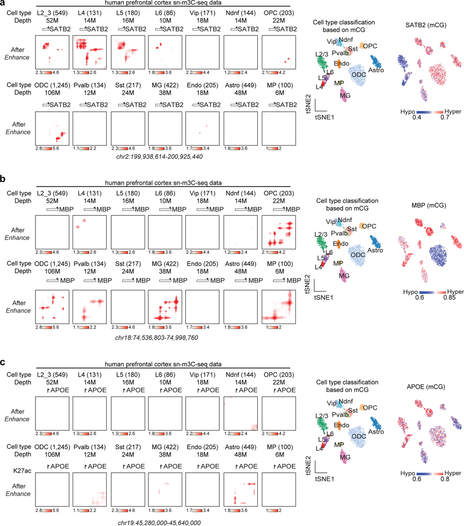
Lastly, we applied DeepLoop to a sn-m3C-seq dataset in human prefrontal cortex (PFC) in which the identities of 14 cell populations are already resolved by DNA methylation profiles⁵². Most cell populations have at least 100 cells and 10M read depth, which is adequate for us to directly observe population specific loop profiles. For example, RORB loop signal are restricted in layers 4/5 but not layers 2/3/6 neurons, which is highly consistent with the DNA hypomethylation signal (Figure 4e–Figure 4f). Similar observations are also made for tissue specific genes SATB2 (layers 2/3/4/5), MBP (ODC/OPC/MG), and APOE (astrocyte) (Extended Data Figure 7).

DeepLoop nominates allelic loops at imprinting or DMR loci

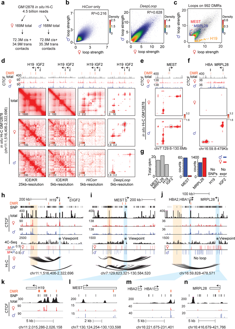
The rest of this manuscript focuses on resolving human allele-specific chromatin loops (AS-loops), which remains a difficult task yet due to the sparse and uneven distribution of heterozygous SNPs. Specifically, GM12878 genome has ~1.7 million heterozygous SNPs (or one SNP per ~1.5kb), which enforces a hard limit for data resolution since only the reads overlapping SNPs are usable. Starting from 4.5 billion GM12878 in situ Hi-C reads⁷, only 337 million (~7.5%) can be assigned to either maternal or paternal genome (Figure 5a); each haploid has ~56 million mid-range cis contacts. We applied DeepLoop to maternal and paternal data independently at 5kb resolution and called top 300K loop pixels from each haploid genome. After enhancement, the R-square between two homologs is improved significantly from 0.216 to 0.628 (Figure 5b), which allows much more robust allelic analyses.

Figure 5. Homolog-specific chromatin interactions are associated with imprinting and DMR.

a, The reads summary of allele-resolved in situ Hi-C data in GM12878 cells. b, Scatterplots comparing the loop strength of all anchor pairs between two haploid genomes. Left: HiCorr Only; right: after DeepLoop. c, Heat scatter showing all loop pixels overlapping 992 DMRs. Loop pixels at three loci with highest allele specificity are highlighted in different colors. Background scatter plots are the union of top 300K loop pixels from both haploid genomes. d, The contact heatmaps of the H19/IGF2 locus. e-f, The contact heatmaps of gene MEST and MRPL28 after DeepLoop. g, Gray bar plot on the left: the RPKM of four genes in GM12878 showing their expression level; bar plots on the right: RNA read counts on the two alleles for each gene. Note that although H19 is expressed, its mRNA sequence does not contain heterozygous SNP for allelic analysis. h-j, The browser tracks for the three loci in d-f. 4C-seq tracks shows the chromatin interactions with the DMR region as viewpoint. Tracks of allelic 4C-seq analysis is included to show the maternal (red) or paternal (blue) preference of 4C-seq signal. Light blue: DMR that anchors allelic loop; light orange: the other anchor of the allelic loop. k-n, zoom-in track views of h-j showing the regions with DMR. The height of browser tracks show ChIP-seq read counts pileup.

The best-known example of AS-loops is at H19/IGF2 imprinting locus. Early studies using allelic 3C-PCR^53–55 and more recently allelic 4C-seq⁵⁶ showed that in mouse cells, a paternally methylated gametic DMR (differentially methylated region) blocks CTCF binding and loop formation (insulator model). We therefore examine the 3,736 loop pixels anchored on all the 992 DMRs previously defined in human GM12878 cells⁵⁷ (colored dots in Figure 5c). Only three loci, including H19, MEST, and MRPL28, have DMR and AS-loops, consistent with the idea that “insulator model” is not a common mechanism for imprinting control⁵⁸. For H19/IGF2, the AS-loops are barely observable from the KR-normalized heatmaps at 25kb-resolution; the ambiguity is worse at 5kb-resolution (Figure 5d, 1^st and 2^nd columns). HiCorr clearly improves the 5kb-resolution bias-correction and allows DeepLoop to output clean maps of AS-loops consistent with the maternal-specific CTCF binding at H19 DMR (Figure 5d, h, k).

We performed 4C-seq using DMRs as viewpoints and confirmed the allelic imbalance of the AS-loops (Figure 5h–Figure 5j). We also examined the allelic imbalance of the CTCF ChIP-seq data at MEST and MRPL28 loci. MEST is a well-known paternally imprinted gene⁵⁹ (Figure 5g). The MEST DMR is close to two CTCF peaks that form a paternal-specific loop (Figure 5e, Figure 5i, Figure 5l); one peak is ~480bp to its closest heterozygous SNP which supports a paternal CTCF binding with marginal significance (10 vs. 4 reads, p = 0.09, Figure 5l). The MRPL28 transcriptional allele-specificity is weak but the loop is highly specific (Figure 5f, g). There is a strong CTCF peak near MRPL28 DMR that presumably anchors the paternal-specific loops (Figure 5f, Figure 5j, Figure 5n). Although the allele-specificity of this CTCF peak is unknown due to the lack of informative SNPs, a small CTCF peak in this region is highly paternal-specific (23 vs. 4 reads, p = 1.6e-4, Figure 5n). Another CTCF peak at the HBA1/2 DMR is also paternal-specific (60 vs. 20 reads, p = 0.007, 1.6e-4, Figure 5m). In fact, the entire region between HBA1/2 and MRPL28 is decorated with stronger paternal CTCF signals (Figure 5j). It should be noted that we are still not sure if MRPL28 is an imprinting locus because it is unclear whether the MRPL28 or HBA1/2 DMRs are gametic DMRs.

DeepLoop reveals chromatin loops that escape X-inactivation

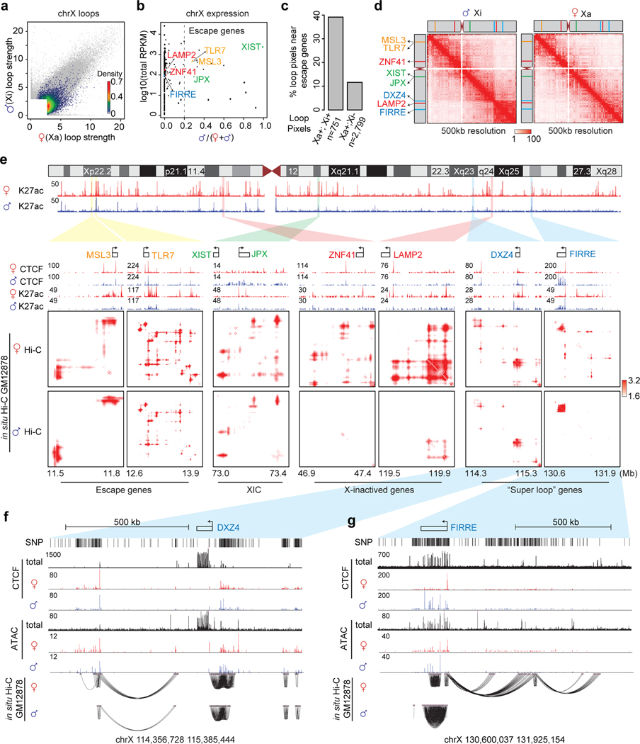
Allelic Hi-C analyses at low-resolution in both human and mouse cells have reproducibly observed the loss of TAD domains and the formation of “megadomain” and ultra-distal “superloops” in the inactivated X chromosome (Xi)^2,7,60–62. But the architectures of Xi and Xa (active X chromosome) have not been compared at sub-TAD loop level. In human GM12878 cells, the paternal chrX is inactive. DeepLoop called 3,550 and 806 loop pixels from Xa and Xi, respectively (Figure 6a), indicating that most chromatin loops are repressed by X-inactivation. Most of the chrX genes are monoallelic except 17 escape genes including the X-inactivation center (XIC) genes XIST and JPX (cutoff P/(M+P) > 0.2, Figure 6b). As expected, escape loop pixels (present in both Xi and Xa) are enriched near the escape genes (Figure 6c, examples in Figure 6e).

Figure 6. Homolog-specific chromatin interactions are associated with X-inactivation.

a, The heat scatter plot of all chrX loops in color. Grey dots in the background: the union of all top 300K loops in both haploid genomes. b, Scatterplot showing the genes expression from the two chrX copies. x-axis: the fraction of RNA reads on paternal alleles out of total from both alleles; y-axis: the RPKM of total expression in log scale; genes of interest in d-e are highlighted in different colors. Dashed vertical line indicates the cutoff to define escape genes. c, Bar plot showing the percentages of “escape loop pixels” (present in both Xa and Xi) or “inactivated loop pixels” anchored to the 17 escape genes (TSS +/− 100kb) defined in b. d, The chrX heatmaps with KR-normalization at 500kb resolution showing the “megadomain”. e, DeepLoop enhanced Hi-C heatmaps are shown for two homologs at 7 representative loci, including escaping loci (yellow), XIC (green), X inactivated loci (red), and Xi megadomain or superloops loci (blue). f-g, Genome browser tracks at DXZ4 and FIRRE loci. The ChIP-seq tracks show raw reads pileup.

We next examine the relationship between chromatin loops and high-order “megadomain” or “superloop” structures in Xi.. DXZ4 is at the boundary of the “megadomain” (Figure 6d) and also form “superloop” with the downstream FIRRE locus^7,63. The gene bodies of both DXZ4 and FIRRE gain CTCF binding in Xi, which may function to anchor the Xi to the nucleolus^61,63,64. Interestingly, we found that the two loci respond differently to X-inactivation. At DXZ4 locus, the chromatin loops, CTCF peaks, and ATAC-seq peaks are invariant between Xa and Xi, suggesting that this locus escapes X-inactivation (Figure 6e,f). In contrast, although the Xi FIRRE gains much strengthened loop pixels within its own gene body, all loops connecting FIRRE to surrounding regions are lost (Figure 6e,g), indicating that FIRRE locus is X-inactivated. Consistent with these observations, FIRRE gains CTCF and ATAC-seq signals in its gene body, but lost CTCF and ATAC-seq signals at promoter (Figure 6e,g). Notably, FIRRE is predominantly expressed from Xa (Figure 6b), also indicating that it is X-inactivated⁶⁵.

Because both DXZ4 and FIRRE form “superloop” but only DXZ4 is at the “megadomain” boundary, our observation suggests that the escape loops near DXZ4 (presumably mediated by cohesin and loop extrusion) is mechanistically coupled to the formation of “megadomain”, but not the “superloop”; other mechanisms (e.g., co-localization to nucleolus) may cause the “superloops”. These results agree very well with a recent study showing that loss-of-cohesin disrupts the Dxz4 “megadomain” but enhances the Dxz4-Firre “-superloop” in mouse cells⁶⁶. Taken together, we propose that opposite to their names, “megadomain” is using a cohesin-dependent looping mechanism while “superloop” is not.

DeepLoop functionally characterizes large heterozygous SVs

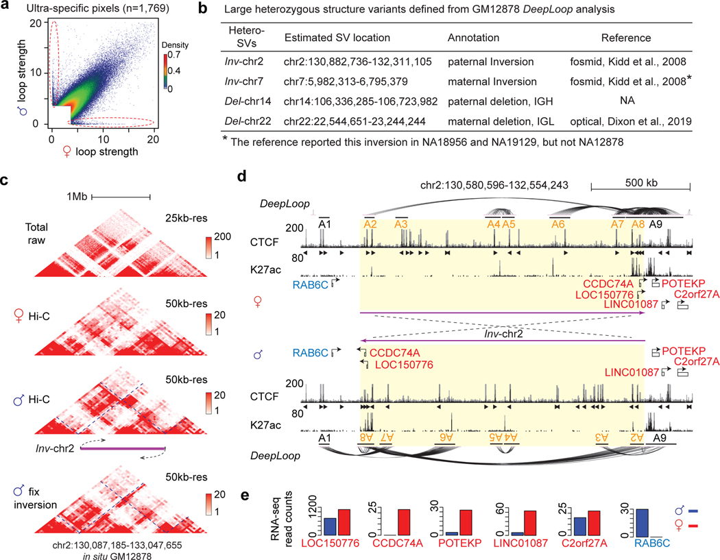
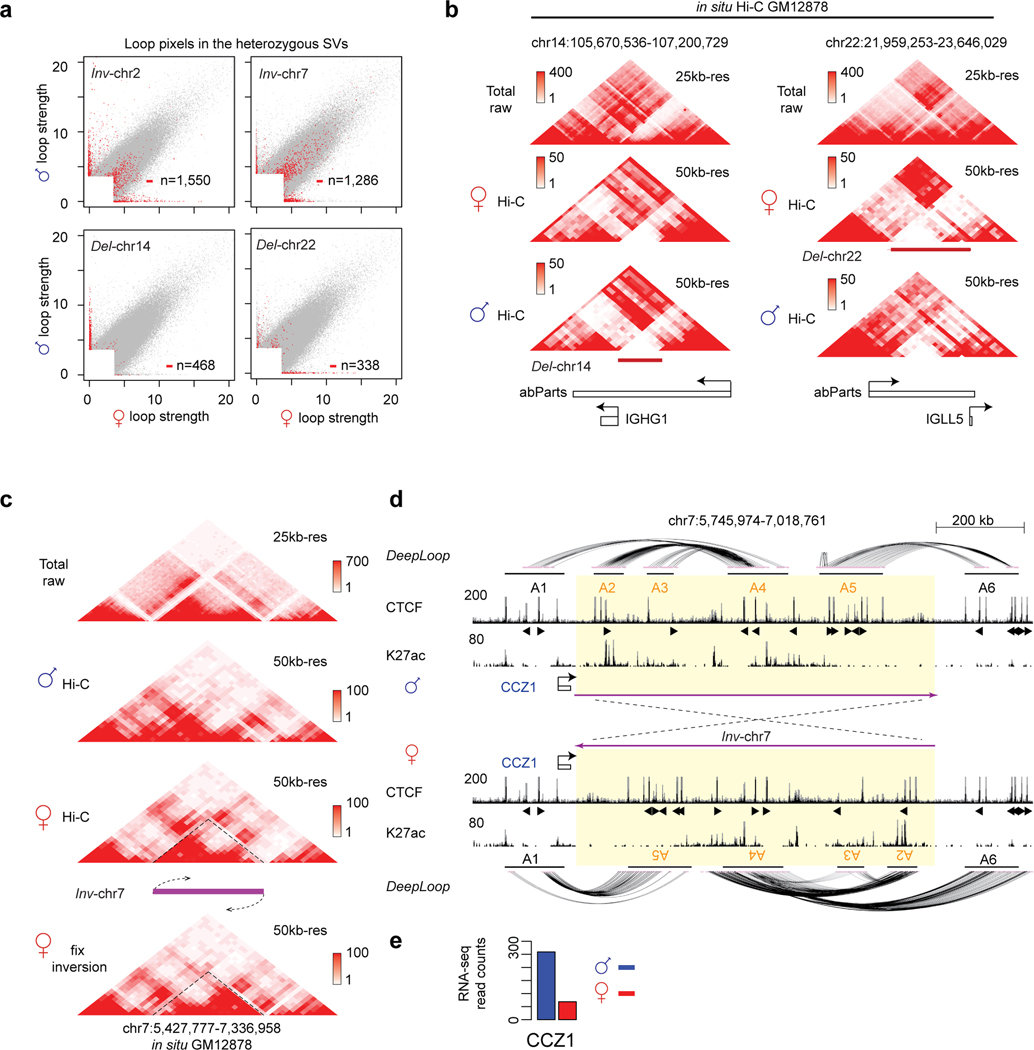
We are intrigued to see many loop pixels with extreme allele specificity (> 10-fold difference, p < 0.01) after DeepLoop but not before enhancement (Figure 5b, circled scatter points in Figure 7a). Interestingly, 1,533 of these 1,769 (87%) ultra-specific pixels are in four regions. Based on the patterns of maternal and paternal contact heatmaps⁶⁷, we concluded that these regions harbor large heterozygous deletions and inversions (Figure 7b–Figure 7c, Extended Data Figure 8a–c). Del-chr14 (~300kb) and Del-chr22 (~600kb) are large heterozygous deletion at the IGH and IGL immunoglobulin loci, consistent with the allele exclusive V(D)J recombination process in B-lymphocytes (Figure 7b and Extended Data Figure 8b). The two inversions are even bigger (Inv-chr2, ~1.4Mb; Inv-chr7, ~900kb) (Figure 7b). The extreme allele-specificity is apparently due to the incorrect distance-bias correction when using reference genome for the SV alleles.

Figure 7. Allelic DeepLoop maps can detect and functionally characterize large heterozygous SVs.

a, Scatterplot showing the ultra-specific loops (in red circles). b, Four large heterozygous SVs containing a majority of the ultra-specific loops. c, The raw contact heatmaps of the Inv-chr2 locus. The “corrected” raw heatmap of the inverted paternal allele is included (“fix inversion”). d, The genome browser track of the Inv-chr2 locus shows CTCF and H3K27ac binding and chromatin loops in the un-inverted maternal allele and the inverted paternal allele. e, Bar plots showing the allelic expression of the genes highlighted in d at the inversion boundaries.

Heterozygous SVs, especially large inversions, are notoriously difficult to detect^68–70. We looked up the four heterozygous SVs in published GM12878 data using various SV-detection tools^53,57,58 (Figure 7b) and found that: (i) neither short- nor long-read whole genome sequencing detected any of the four SVs^67,71; (ii) optical mapping detected Del-ch22 at IGH locus⁶⁷; (iii) a previous Hi-C analysis did not detect any of these SVs because the study assumes homozygous genome and only performed 1Mb-resolution analysis⁶⁷; (iv) the conventional fosmid subcloning-based method detected Inv-chr2 but had no knowledge about its heterozygosity⁷²; (v) the fosmid method detected Inv-chr7 in two independent NA18956 and NA19129 genomes but not NA12878, suggesting that Inv-chr7 is a recurrent SV in the human population⁷². Taken together, allelic DeepLoop analysis appears to be a promising approach to detect large heterozygous SVs.

To correctly map the chromatin loops affected by the inversions, we adjust the orientation of the inverted allele using the annotated inversion coordinate⁷² and redid the DeepLoop enhancement (Figure 7c,d and Extended Data Figure 8c,d). For Inv-chr2, the paternal inversion breaks apart an enhancer cluster at 3’ boundary that is heavily inter-connected in the maternal genome (A7–9 in Figure 7d). Genes connected by this enhancer cluster, including LOC150776, CCDC74A, POTEKP, LINC01087, and C2orf27A, are all downregulated in the inverted paternal genome (Figure 7d,e). On the other hand, Inv-chr2 moved half of the 3’ boundary enhancer cluster (A7–8) to the 5’ boundary; new loops form across the 5’ boundary between A1 and the inverted A7–8 anchors (Figure 7d). The new loops can explain the paternal expression of RAB6C gene (Figure 7e). Similarly, Inv-chr7 also rewires the DNA loops which explains the paternal-specific CCZ1 expression (Extended Data Figure 8d,e). These results demonstrated that DeepLoop can detect and predict the regulatory effects of large heterozygous structure variants, which may link to diseases or phenotypes^73,74.

DeepLoop pinpoints SNPs that affect loops and transcription

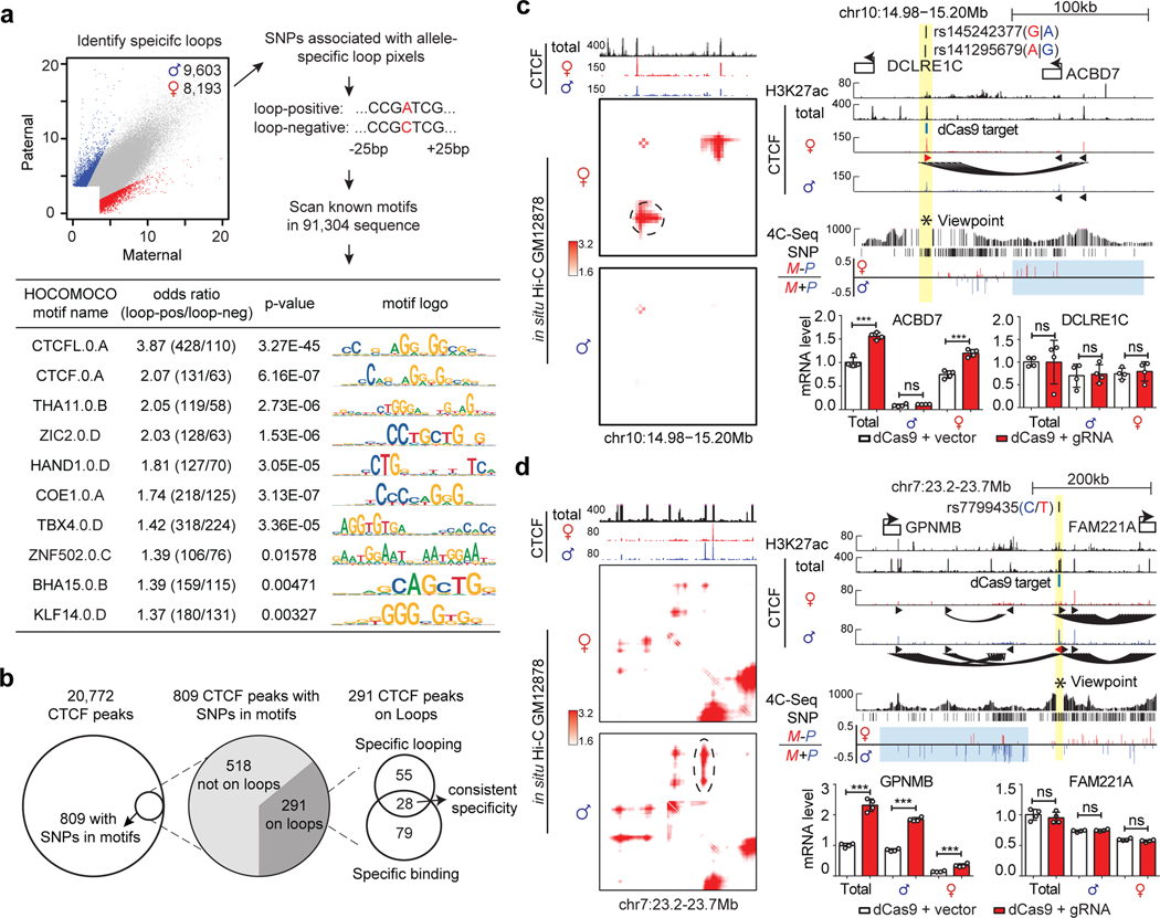
Lastly, we investigate the impacts of heterozygous SNPs on the chromatin loops. After excluding the AS-loop pixels associated with imprinting, X-inactivation, and SVs, we use a simple two-fold cutoff and called thousands of AS-loop pixels at 1,959 loci (Figure 8a). These loop pixels contain 91,304 heterozygous SNPs for which “loop positive” and “loop negative” alleles can be unambiguously defined. CTCFL and CTCF are the top two motifs enriched in “loop positive” alleles, proving the feasibility to resolve the genetics of loops with DeepLoop. Other motifs are also enriched, such as the COE1.0.A bound by the B-lymphocyte specific transcription activator EBF1, and a motif bound by KLFs which have been shown to regulate loops in other cell types^75–77 (Figure 8a). Further studies are necessary to verify the loop-regulatory functions of individual SNPs and their cognate TFs.

Figure 8. Allelic DeepLoop maps can pinpoint common SNPs that affect chromatin loops.

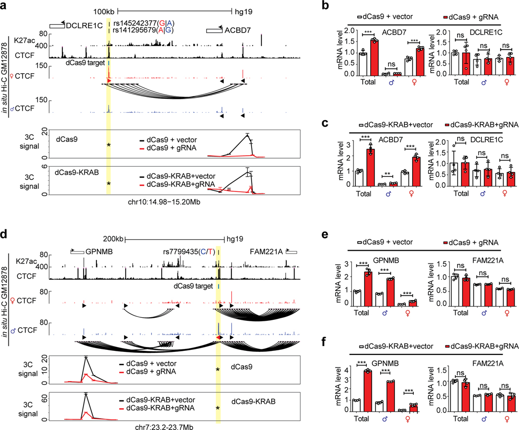
a, Flowchart showing the de novo motif findings associated with allele-specific chromatin loops. The scatterplot highlights the allele-specific loops. The 51-base sequences (25bp up/down) around the SNPs are used to scan for motifs significantly enriched in the loop-positive alleles. Fisher’s exact test was performed to measure the motif enrichment. b, Summary of the procedure to identify causal SNPs for allele specific CTCF loops and TF occupancy. c-d, Using “insulator epigenome editing” to validate the transcription regulatory functions of two selected allelic-specific CTCF loops. Both contact heatmaps and genome browser tracks are included to show the locations of SNPs, the specific CTCF peaks and DNA loops. 4C-seq tracks shows the chromatin interactions with the SNP region as viewpoint (highlighted in yellow). Tracks of allelic 4C-seq analysis show the maternal (red) or paternal (blue) preference of 4C-seq signal. The regions of interest are highlighted in light blue. The bar plots show the changes of nearby gene expression with allele-specific RT-qPCR upon CTCF-blocking with dCas9. N=2 biologically independent experiments. All data are presented as means ± SEM from 4 replicated experiments. **p < 0.01, ***p < 0.001. NS, no significant difference. Two-sided Wilcoxon test. (More results in Extended Data Figure 10).

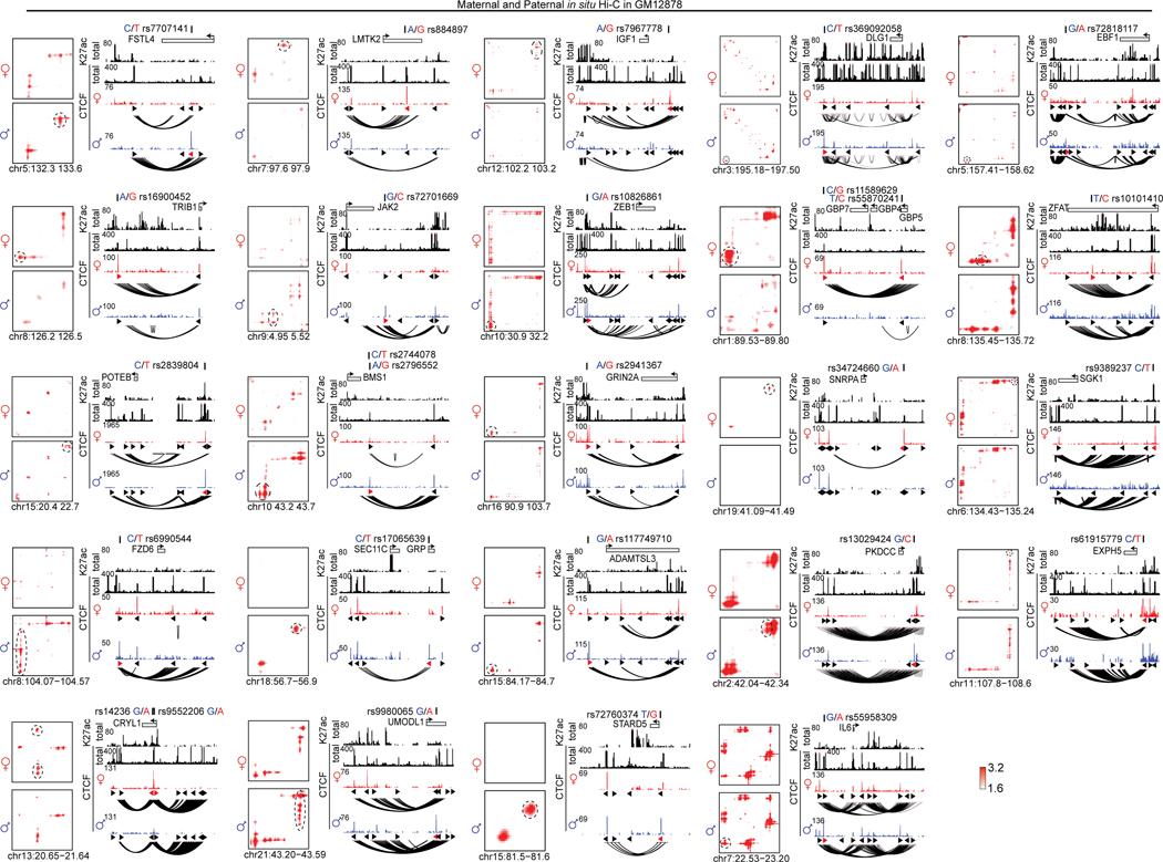
We next seek to map the causal SNPs of the CTCF AS-loops. In GM12878 cells, 809 (3.9%) of all 20,772 CTCF peaks have heterozygous SNPs in their cognate motifs (Figure 8b), among which we narrowed down to 28 highly credible AS-CTCF peaks (involving 30 SNPs in 26 loci) anchoring consistent AS-loops. For two selected loci, we confirmed their allele specificity with 4C-seq (Figure 8c,d). The snapshots of the rest 24 loci in Extended Data Figure 9.

We also use a dCas9-based insulator editing approach^78,79 to test if the AS-CTCF loops affect transcription in cis. With sgRNAs precisely targeting the cognate CTCF motifs, both dCas9 and dCas9-KRAB proteins can abolish the CTCF loops of interest (Extended Data Figure 10a,d). In the first example (Figure 8c, Extended Data Figure 10a–c), the maternal alleles of rs141295679 and rs145242377 (both SNPs are within the same CTCF motif) are associated with stronger CTCF binding and a maternal loop encompassing the ACBD7 gene. Blocking the loop increases the maternal expression of ACBD7 but does not affect a control gene outside the loop (DCLRE1C). In the second example (Figure 8d, Extended Data Figure 10d–f), the paternal allele of rs7799435 form a strong CTCF loop encompassing GPNMB gene. Blocking the paternal CTCF loop also increases the paternal GPNMB expression but does not affect FAM221A gene from a different neighborhood. These examples demonstrated that allelic DeepLoop analysis can pinpoint common SNPs that regulate gene expression by directly affecting DNA looping.

Discussion

DeepLoop is a novel framework that enhances Hi-C ratio heatmaps (instead of contact heatmaps) without distance effects. Because bias-correction and signal-enhancement are carried out in two independent modules, each module can be modified or upgraded without affecting each other. DeepLoop is a universal tool that can be applied to different Hi-C data types if HiCorr has been properly adjusted. The lower limit of read depth is ~10M mid-range cis contacts, typically can be obtained from 50~100M total reads. Nearly all published Hi-C datasets have adequate reads for DeepLoop reanalysis. Existing single cell Hi-C technologies can yield enough reads from a few dozen cells. DeepLoop allowed us to map the human AS-loops and revealed the genetic and epigenetic determinants of chromatin loop variations. We have setup a public webapp to visualize the DeepLoop-enhanced heatmaps for ~40 datasets mentioned in this study. In summary, DeepLoop makes Hi-C a robust and affordable approach to reveal the genome organization at sub-TAD loop level.

Methods

No ethical approval was needed.

Experiments

Hi-C on H9 cells

H9 cells (WiCell, #WA09) were maintained in mTeSR1 medium (StemCell Technologies, Cat#05850) on plates coated with hESC-Qualified Matrigel (Corning, Cat#354277) before harvested for Hi-C. After removing differentiated colonies by handpicking, the cells were digested to single cells with Accutase (Innovative cell technologies, Cat#AT104) and then fixed with 1% formaldehyde. Hi-C was performed according a published protocol⁶. Firstly, the fixed cells were lysed with cell lysis buffer containing 10 mM Tris-Cl pH8.0, 10 mM NaCl, 0.2% NP-40 and 1x protease inhibitor cocktail (Roche, Cat#11873580001) with douncing in between. The nuclei were then collected and digested with HindIII (NEB, Cat# R3104M) in 1x cutsmart buffer (NEB, Cat# B7204S) for overnight at 37°C. The digested fragment ends were then labelled with Biotin-14-dCTP (Thermo Fisher, Cat#19518–018) using DNA polymerase I, large fragment (NEB, Klenow, Cat#M0210L). After biotin labelling, the nuclei were subjected to proximity ligation using T4 DNA ligase (Invitrogen, Cat# 15224–090) in large volume of 7.5ml. The ligated nuclei were then collected by spinning down at 2,500g for 5 minutes followed by DNA extraction with phenol-chloroform after reverse-linking with proteinase K for overnight. The purified DNAs were first quantified with Qubit dsDNA HS assay kit (Invitrogen, #Q32854) and then treated with T4 DNA polymerase (NEB, Cat#M0203L) to remove the unligated DNAs. To generate fragments that can be sequenced, DNAs were then subjected to sonication using a Covaris S2 sonicator under the following condition, duty cycle 10, intensity 4, cycles/burst 200 for 55 seconds. The resulted DNAs were end repaired using DNA End-Repair kit (Lucigen, Cat#ER81050). Then, an “A” was added to the ends of each fragment using Klenow fragment (3’→5’ Exo-) (NEB, Cat#M0212L). 300–500bp fragments were then selected using homemade Sera-Mag beads. C1 Streptavidin Beads (Invitrogen, Cat#650.02) were used to pull down the biotin-labelled ligates. After pulling down, the beads were washed for 3 times with 400 μl of 1x binding buffer (5mM Tris-Cl, pH8.0, 0.5mM EDTA and 1M NaCl) followed by twice with 100 μl of 1x ligation buffer (NEB, #B0202S). Illunima Truseq adapters were then ligated using T4 DNA ligase (NEB, Cat#M0202L). 6pmol of paired end adapters were used for 1μg DNA. The resulted DNA were then PCR amplified using short primers (Supplementary table 7). The final libraries were sequenced on Illumina HiSeq 3000 platform.

4C-seq

The 4C-seq was performed following a published protocol⁸⁰. First, 3–5 million cells were harvested and fixed with 2% formaldehyde, and then quenched with 125 nM glycine. The fixed cells were then lysed with a cell lysis buffer, which contains 50 mM Tris-Cl pH7.5, 150 mM NaCl, 5 mM EDTA, 0.5% NP-40, 1% Triton X-100 and 1x protease inhibitor cocktails (Roche, Cat#11873580001), for 20–30 minutes on ice. After lysing, the nuclei were collected by spinning down at 2,500g for 5 minutes at 4°C followed by washing with 1x restriction enzyme buffer once. The nuclei pellets were then resuspended in 1x restriction enzyme buffer and treated with 0.3% SDS for 1 hour at 37°C under shaking, followed by another hour with 2.5% Triton X-100. Chromatin digestion was then done by incubating the samples with designated restriction enzyme at proper temperature for overnight while rotating in an airbath. The restriction enzymes used for each locus were listed in Supplemental Table 7. After digestion, heat inactivation at 65°C was applied to inactivate the enzymes and the nuclei were then subjected to ligation with 50μl of T4 DNA ligase (Invitrogen, Cat# 15224–090) in a 7ml ligation solution at 16°C for overnight. Reverse-linking was then performed by treating the samples with proteinase K to get the proximity ligated DNA. The purified DNAs were quantified and subjected to the secondary restriction enzyme digestion, roughly 1 unit of restriction enzyme for 1μg DNA, at the suggested temperature for overnight. After inactivation of the restriction enzymes, the samples were then self-ligated with T4 DNA ligase. The ligated DNAs were recovered with Sodium Acetate and ethanol and quantified with Qubit dsDNA HS assay kit (Thermo Fisher, Cat# Q32851). The 4C-templates were then amplified with designed primers to generate libraries for sequencing. We modified the primer system to make it compatible with Illunima Nextera system using two sequential PCRs. The locus specific inverse PCR primers are listed in the Supplemental Table 7. For each locus, the 4C templates were amplified with locus specific primers using 200ng template in each reaction, and products from 5 parallel amplifications were pooled to generate the final 4C library. A 50 μl PCR product aliquots were purified with homemade Sera-Mag beads. And one fifth of the purified DNAs were used for the second PCR using primers N7xx and N5xx that are the same as Illumina Nextera sample preparation primers. The final products were then purified and subjected to sequencing. The reads for the first cutting site were used for data analysis.

Cloning

For the gRNA expression vector, we use a pX332-original plasmid gifted from the laboratory of Joanna Wysocka (Standford)⁸¹, which contains a mCherry expression cassette. The dCas9 and dCas9-KRAB expression vectors described in this study were generated on a backbone of Cas9 expression vector: pX330 plasmid (Addgene; plasmid 42230) by using In-Fusion cloning method. Both of the dCas9 and dCas9-KRAB genes were amplified from pHAGE EF1α dCas9-KRAB (Addgene; plasmid 50919) with PCR and cloned separately into the AgeⅠ and EcoRⅠ sites of pX330 plasmid, replacing the Cas9 ORF. The detailed information for primers can be found in Supplementary Table 7. All sgRNAs in this study were designed on CCTop-CRISPR/Cas9 target online predictor^82,83 and manually picked.

GM12878 Cell culture and nucleofection

The GM12878 cells were maintained in RPMI 1640 medium (Gibco, Cat#11875–085) supplemented with 15% FBS (Gibco, Cat#16000–044) and 1% pen/strep (Gibco, Cat#10378–016). Cells were split and seeded at 300k cells per ml in fresh medium the day before nucleofection. About 4 million cells were prepared for each nucleofection. Briefly, cells were pelleted by centrifuging at 90g for 5min and then resuspended in nucleofection reagent as suggested by the manual (Lonza, SF cell line 4D-Nucleofector X kit, Cat#V4XC-2024). For each reaction, about 5–7ug designated plasmids (dCas9 or dCas9-KRAB combined with pX332-gRNAs, each ~2–4μg) were applied. The nucleofection was done on a 4D lonza nucleofector with program CM-137. Cells were then stand and recovered for 24 hours in the cell culture incubator before harvested for RNA extraction or 3C analysis.

RNA extraction and RT-qPCR

RNA was extracted with Trizol from the nucleofected cells following the standard protocol. cDNAs were generated by reverse transcription using M-MLV Reverse Transcriptase (Invitrogen, Cat# 28025013) following the manual. qPCR was done in triplicates.

3C-qPCR

After nucleofection, the cells were harvested for 3C-assay by fixing with 1% formaldehyde. Cells were lysed using a cell lysis buffer (10mM Tris-Cl, pH7.5, 10mM NaCl, 0.2% NP-40 and 1X proteinase inhibitor cocktail) with total 30 times of douncing in between on ice for about 20 minutes. Cell nuclei were then pelleted by centrifuging at 2,500g for 5 minutes at 4°C. After that, the nuclei were digested with MboI (NEB, Cat#R0147M), 400U for about 4 million cells, at 37°C overnight. After heat inactivation of MboI, the proximity ligation was done with T4 DNA ligase (Invitrogen, Cat#15224–025) at 16°C for overnight. The proximity ligated chromatins were reverse linked by treatment with proteinase K at 65°C for overnight and then purified by phenol: chloroform. To generate random ligation control for 3C-qPCR, we pick BAC clones covering the two anchors of the loop of interest (list of BAC clones in Supplemental Table 7) and perform 3C procedure on the DNA prepared from BAC clones.

Sequencing data analysis

Hi-C data mapping, filtering, and normalization

Conventional Hi-C

Because some of conventional Hi-C libraries are sequenced with paired-end 36bp (e.g. human tissue datasets), for consistency and convenience purpose we trimmed all conventional Hi-C data to 36bp long. Each end of the raw reads was mapped separately to the hg19 (for human), mm10 (for mouse) reference genome using bowtie (v1.1.2)⁸⁴. Sam files were then paired with an in-house script. After removing PCR duplications, we first discarded the reads with both ends mapped to the same HindIII fragments as invalid pairs. All remaining read pairs represent two different HindIII fragments in cis. Since cut-and-ligation events are expected to generate reads within 500bp upstream of HindIII cutting sites due to the size selection (“+” strand reads should be within 500bp upstream of a HindIII site, and “-“ strand reads should be within 500 bp downstream a HindIII site), we only kept read pairs with both ends satisfying these criteria. We next split all the remaining reads into three classes based on their strand orientations (“same-strand”, “inward”, or “outward”). We kept the “inward” read pairs if the distance between two reads is more than 1kb, and the “outward” read pairs if the distance between two reads is more than 25kb. Then we merged the filtered “inward”, filtered “outward” and “same-strand” as the cis reads pair. The HiCorr “HindIII” mode was used to get bias corrected 5kb anchor loop files from cis and trans fragment read pairs.

In situ Hi-C and micro-C

The full length reads (150bp for in situ GM12878) were used for alignment to enable more reads overlapping SNPs for allele resolved analysis. After removing PCR duplicates and read pairs classification, we filtered out the “outward” read pairs with distance less than 5kb, and “inward” read pairs with distance less than 1kb. Then the filtered read pairs were mapped to Mbol fragment pairs and HiCorr “Bam-process-DpnII” mode was used for bias correction. The H1 micro-C processing followed the similar steps, we used 5kb bins to map read pairs, and Juicebox (v1.18.08)85 “pre” to convert 5kb bin pairs to “hic” format and ran KR normalization. Then we dumped the contact pairs and further did distance correction with in-house scripts. In brief, we split all the contact pairs within 2Mb by loop distance into 400 groups with 5kb as interval. In each distance group, the KR normalized value was normalized by the average values within the same group. Here, we called the normalized value from KR normalization and distance correction as “KR-ratio”.

Single cell Hi-C preprocessing

The processed DpnII fragment contacts files for 4,098 mouse embryonic stem cells were downloaded from original study (Supplementary Table 1). The fragment pairs were then liftover from mm9 to mm10. The number of cis contacts within 2Mb was used to rank the cells. We took top-ranked cells of a certain number (1~92) and merged the fragment contacts files for cis and trans separately and mapped to ~10kb anchor pairs. HiCorr “DpnII” mode was used to correct bias at the anchor level. The “contact read pairs” files for human prefrontal cortex sn-m3C-seq and the cell type labels identified from the methylation profiled in the same cell were downloaded from original study (Supplementary Table 1). We aggregated the cells from the same cell type, filtered reads pair as in situ Hi-C steps and further mapped the read pairs to DpnII fragment pairs. Due to the sparsity and limited depth of each cell type, we further converted fragment pairs to ~10kb anchor pairs. For each cell type, the merged cis anchor contact file and trans anchor pairs were taken as input to run HiCorr “DpnII” mode.

4C-seq

The 4C-Seq data were analyzed using pipe4C (v1.1.3)80 to generate bam files and wig files for visualization.

Allele-specific mapping for Hi-C, ChIP-seq, RNASeq and 4C-seq

We first masked hg19 reference genome with SNPs downloaded from original study (Supplementary Table 1) and built index for bowtie2 (v2.2.6)86 and Hisat2 (v2.1.0) 87.

Hi-C

Each end of the raw reads with the full length (150bp) was mapped separately to the masked hg19 genome by bowtie2 (v2.2.6). SNPsplit v(0.3.4)88 was used to assign mapped reads in bam files to two alleles using the SNP information. The read pairs filter step is the same as in situ Hi-C (see section above). HiCorr “DpnII” mode was used for bias correction. LoopEnhance model trained by 50M data was used to enhance the two 5kb-resolution contacts data from the two alleles. The top 300,000 loops from two datasets were combined and then the loops with at least two-fold difference between the enhanced loop strength of the two alleles were defined as allele-specific loops. The ultra-specific loops were defined by 10-fold.

ChIP-seq

The FASTQ files were mapped to the masked hg19 genome by bowtie2 (v2.2.6). SNPsplit (v0.3.4) was used to assign mapped reads in bam files to two alleles using the SNP information. macs2 (v2.2.7.1)89 was used to call peaks.

RNA-Seq

The FASTQ files were mapped to the masked hg19 genome by Hisat2 (v2.1.0), SNPsplit (v0.3.4) was used to assign mapped reads in bam files to two alleles using the SNP information. We used FeatureCounts (v1.6.1) to summarize the mapped reads for each gene across samples. The reads on the same allele from different samples were merged. The binomial test was performed to calculate p-value comparing expression level between two alleles for each gene (background possibility is 0.5). The X-inactivation causes the imbalance of gene activity between $X_a$ (maternal) and $X_i$ (paternal) genomes, the escape genes were defined as the genes with ratio over 0.2.

$$ratio=\raisebox{1ex}{${expr}_{Xi}$}\!\left/ \!\raisebox{-1ex}{${expr}_{Xi}+{expr}_{Xa}$}\right.$$

${expr}_{Xi}$ is the paternal ($X_i$) expression of the gene, ${expr}_{Xa}$ is the paternal ($X_a$) expression of the gene.

4C-Seq

The 4C-Seq data were analyzed using pipe4C (v1.1.4) to generate bam files and wig files for visualization. We further converted bam file to bed format and extracted the reads overlapping SNPs and split them to maternal and paternal bed files. For each SNP, we summarized the overlapped reads on maternal and paternal genomes and calculated the allele imbalance using the formula below and visualized it on UCSC genome browser.

$$Alleleimbalance=\left(M-P\right)/M+P$$

$M$ is 4C reads assigned to maternal genome on each SNP, $P$ is 4C reads assigned to maternal genome on each SNP.

Data Representation and model structure in DeepLoop

Data Representation

To train deep learning models on Hi-C contact matrices, we need to represent the data in a way that is more computationally tractable than holding each full chromosome matrix in memory. We took each full chromosome matrix and split it into non-overlapping equally sized sub-matrices that lie within the 2Mb band. For a single genome using our selected sub-matrix size of 128×128, we used on average ~18,000 unique sub-matrices per replicate when training a model, though we use random cropping and shifting to further augment the training dataset. Once the model was trained, each of these sub-matrices was passed into the model separately and the full chromosome matrix was reconstructed from the outputs of the trained model.

LoopDenoise

Denoising Autoencoders

A convolutional autoencoder⁹⁰ is a type of neural network that consists of an encoder function and a decoder function. The encoder maps an input vector to a lower dimensional latent representation using successive convolution layers combined with some form of dimensionality reduction such as pooling layers or strided convolutions. The decoder then maps this representation to a reconstructed vector using transpose convolutions or some other form of up sampling. Autoencoders altogether can be thought of as a function $f_{\theta }$parameterized by $\theta$, which maps each input vector $X_i$ from a given dataset to a reconstructed vector $f_{\theta }\left(X_i\right)$. Classical autoencoders try to learn an approximation to the identity function by using the input vector as the training target⁹¹. That is, for a dataset $X$ the model tries to minimize the loss between each input vector and the reconstructed output. Mean squared error is commonly used as the loss function:

$${\theta }^{\mathrm{*}}={argmin}_{\theta }\left[\frac{1}{n}{\sum }_{i=1}^n{\left(f_{\theta }\left(X_i\right)-X_i\right)}^2\right]$$

Denoising autoencoders are a specific type of autoencoder that attempt to learn a mapping from noisy input vectors to clean, ground truth targets⁹². Contrary to classical autoencoders, these denoising models attempt to minimize the loss between some target vector $\widehat{X_i}$and the reconstructed output:

$${\theta }^{\mathrm{*}}={argmin}_{\theta }\left[\frac{1}{n}{\sum }_{i=1}^n{\left(f_{\theta }\right(X_i)-{\widehat{X}}_i)}^2\right]$$

This target vector has some desirable properties such as being noise free or higher resolution than the input vector. Building a denoising autoencoder usually involves starting from the clean ground truth data as the target vectors and corrupting them to generate the input vectors. If the goal of the model is to be robust to noise, we could corrupt the ground truth data by adding random noise. However, in the case of Hi-C contact matrices the data already contains noise, thus training a convolutional autoencoder to denoise Hi-C data requires some more desirable training target. We obtain cleaner training targets by statistically filtering out insignificant signals from high depth data using biological replicates.

Training set

For model training, we picked a published HindIII-based Hi-C dataset in human fetal cerebral cortex²⁴. The data were generated for three donors; every donor has one library from cortical plate (CP) and one library from germinal zone (GZ). All 6 libraries have roughly the same sequencing depth, and the pooled data of all 6 libraries has ~470 million mid-range cis contacts (Supplementary Table 2). We disregard the difference between CP and GZ and split the Hi-C data into three biological replicates: each replicate has 140~150 million mid-range cis contacts combining the CP and GZ libraries from the same donor. We applied HiCorr to each of the three replicates and extracted ~18,000 submatrices at 5~10kb resolution (within the 2Mb range) from every replicate as training sets

Training target

The training target for LoopDenoise should contain significant and reproducible signals with as little noise as possible. To generate these targets, we pooled all libraries together and applied HiCorr; the heatmaps from pooled data shall be less noisy due to higher sequencing depth (Figure 1c). HiCorr provides the p-values for every pixel in the heatmaps from individual replicates and the pooled data. We then removed pixels from the pooled heatmaps with p-value > 0.05 due to the lack of signal enrichment. We then required the remaining pixels to be significant (p-value < 0.05, negative binomial test) in at least one of the biological replicates. The resulting pixels are used as the ground truth training target in our convolutional autoencoder. All the rest pixels are assigned zero values indicating no interaction. Even though these training targets are not completely noise free, results show that our model is able to learn a meaningful latent representation for the true loop signals and is able to output Hi-C sub-matrices that are even cleaner than the training target used. This is likely because the model is forced to learn some average of the noise-free matrices that could explain the noisy observation, rather than learning the perfect mapping to our training target which is not noise-free.

Model Structure

The encoder of LoopDenoise (Figure 1a and Extended Data Figure 1a) consists of two instances of a convolution layer followed by a rectified linear unit (ReLU) activation function and a max pooling layer. The decoder half of LoopDenoise consists of two transpose convolutions followed by a final convolution layer and ReLU activation. Each convolution layer has 8 filters except for the final layer, which only has 1 filter to return the correct number of output channels. The convolution layers in the encoder as well as the final convolution layer use a filter size of 13×13 and the transpose convolutions in the decoder use a filter size of 2×2. The max pooling layers act on a 2×2 region, therefore after each pooling layer in the encoder, the size of the input is halved. For each transpose convolution layer, the size of the input is doubled, giving us the same size output as the input. We applied zero-padding to the edges of each input sub-matrix to ensure that the output size of each convolution or transpose convolution remains unchanged. The output of each convolution layer with ReLU activation was computed as follows:

$$h_i\left(x\right)=max(0,w_i\mathrm{*}\mathit{x}+{\mathit{b}}_{\mathit{i}})$$

where we define the discrete convolution operation * as the weighted sum of the neighboring pixels using weights $w_i$ as the convolution kernel, $b_i$ as the bias and x as the input matrix—either a Hi-C sub-matrix for the first layer, or the output of a previous layer for subsequent layers. This operation was performed at every pixel of the input matrix by using a stride value of 1 to move the convolution window across the input space one pixel at a time. In the transpose convolutions, we performed the same mathematical operation, but we transformed the input by inserting padding between the input values to simulate a fractional stride value, which therefore maps each pixel to multiple different values, increasing the size of the input matrix to perform the up sampling necessary in the decoder.

Model Training

The model was trained by minimizing the mean-squared-error (MSE) of the reconstructed outputs and the combined targets using the Adam⁹³ optimizer with a learning rate of 0.001 and default hyperparameters We used a sub-matrix size of 128×128 and a batch size of 4 training for 50 epochs. Three normalized CP-GZ merged replicates were used for training and chromosomes X and Y were ignored during training. When training this autoencoder architecture, the MSE did not reach zero. This would indicate that our model is overfitting to our training targets and has only memorized the mapping from inputs to targets without learning a useful latent representation that generalizes to novel examples. To avoid this, we used GM12878 replicates as a validation dataset and monitored both the loss and reproducibility on this validation set to ensure that the model would successfully generalize.

Hyperparameter Exploration

To find the optimal model for denoising we trained multiple models with different hyperparameters on the human fetal brain datasets and validated the model using the GM12878 replicates. We tested different filter sizes to see if including more information from neighboring regions leads to improved performance. We evaluated the reproducibility among the training and validation replicates to decide on the optimal filter size of 13×13. We also tested the performance of using a stride value of 2 in the convolution layers of the encoder instead of pooling layers. This would perform the same amount of dimensionality reduction, but each convolution would potentially give us less information than when using pooling layers. We found that max pooling layers slightly improved reproducibility on our training and validation datasets. This makes sense because using a stride value of 2 means that some pixels are never convolved with their neighbors before the dimensionality reduction step and thus the model loses information about certain regions. Compared to a convolution with stride value of 1 followed by max pooling, we capture the full relationship between each pixel and its surrounding region then select the max value among a small group of these pixels. The latter method is more specific about the information that is forgotten when performing dimensionality reduction whereas the former method using a stride value of 2 without pooling randomly loses information based on the location of each pixel.

LoopEnhance

Model Structure

The U-Net architecture (Figure 2a) is a fully convolutional network similar to but much larger than the convolutional autoencoder used in the denoise model. It contains an encoder and a decoder with the main addition being skip connections which concatenate feature maps from each stage of the encoder to each corresponding stage of the decoder. The goal of these skip connections is to maintain the localization and different scales of features when up sampling during the decoder path. Since the receptive field of the convolutions at the final layer of the encoder are very large compared to the size of our input sub-matrices, we found that deep convolutional autoencoders without these skip connections produce very cloudy/blurry signals while concatenating feature maps across the different depths of the model yields more precise signals in the output. The encoder of LoopEnhance contains 10 convolution layers with four pooling layers. Our model has a depth of 4 because it has four ‘blocks’ of convolutions followed by dimensionality reduction steps. The input is a Hi-C sub-matrix of size 128×128. We successively applied two convolution layers with ReLU activation followed by a pooling layer to produce final feature maps with dimensionality 64×8×8=4096. Since we use a U-Net architecture, we also keep the feature maps at each depth of the network. The convolution layers in the first block of the model used 4 filters and this number of filters is doubled at each depth, eventually reaching the 2⁶ = 64 filters found in the final convolution layer. The decoder of LoopEnhance consists of 13 convolution layers with four up-sampling layers. The up-sampling layers are instances of an up-convolution function which simply turns each pixel into a 2×2 region of identical values, then applies a convolution layer with ReLU activation. In practice, this is very similar to a transpose convolution. However, in deep networks transpose convolutions can propagate padding artifacts to the output of the model. Following each up-sampling layer, we applied two convolutions with ReLU activation. The number of filters is now halved after each up-sampling layer starting at 64 filters following the latent encoding and eventually reaching 4 filters. After the final up-sampling layer and its following two convolutions, we applied one final convolution layer with 1 filter and ReLU activation to obtain an output with a single channel.

Model Training

The input to the model is a low depth normalized Hi-C submatrix and the training target is the corresponding denoised high depth normalized submatrix obtained using the denoise model. This is the main distinction between our model and previous works such as HiCPlus²⁰ and HiCNN²¹. Zhang et al note that training a neural network to map low depth Hi-C data to high depth data assumes that the high depth target used is the ground truth. Though many deep learning models are able to distinguish between noise and true signals, the natural variations among Hi-C replicates introduce multiple valid explanations for each low depth input. The increased replicate reproducibility achieved by LoopDenoise facilitates training LoopEnhance by using a ground truth target with less noise and variation. Our model minimizes the mean squared error between the enhanced output and the denoised high depth targets. We also used a larger submatrix size of 128×128 compared to HiCPlus and HiCNN which used 40×40. The larger submatrix size allows our model to map each input submatrix to a richer scale of features while still using minimal padding in the convolution layers. Since our model is a fully convolutional network, once it is trained it can enhance submatrices of any size, though we recommend using the same size that was used during training as padding artifacts are possible with small submatrix sizes.

Hyperparameter Exploration

To find the optimal model for enhancing low depth contact matrices, we trained multiple models with different hyperparameters on the 10% down sampled CP-GZ merged replicates and validated the model using down sampled GM12878 replicates. We tested different filter sizes to see if including more information from neighboring regions leads to improved performance. Like HiCPlus20, we found that larger filters do improve performance to an extent; filters larger than 9×9 showed no significant improvements so we decided on a final filter size of 9×9.

Hi-C data visualization

Heatmaps were used to visualize Hi-C contact profiles. The color scales for heatmaps (raw, expected, ratio) were selected based on the contact matrix. The brightness of pixels in raw, ratio, and DeepLoop heatmaps represent different things, we use different strategies to determine the color scales:

1. Raw heatmaps represents read counts; the brightest red color indicates the 98^th percentile of the contact matrix. Color is proportionally scale-down to 1 read (white).

2. HiCorr heatmaps represents ratios; the brightest red color indicates at least 2-fold enrichment. Color is proportionally scale-down to 1-fold (no-enrichment).

3. DeepLoop heatmaps outputs “transformed fold-change” that only represents relative levels of signal enrichment, i.e., value of 1-fold may no longer be real cutoff for no-enrichment. We therefore set the brightest red color being the lower-limit of the top 300K pixels genome-wide. Color is proportionally scale-down to half of that lower limit or 1-fold, whichever is bigger.

The loop curves in the figures are from UCSC Genome Browser by uploading the top 300K loops in the “biginteract” format. The triangle heatmaps are from UCSC Genome Browser⁹⁴ by uploading the “hic” file generated by Juicebox.

Data Availability

Accession numbers for third party data used in this study can be found in Supplementary Table 1. The raw data of H9 Hi-C and 4C-seq generated in this study and reanalyzed published data can be found in accession number GSE167200. The 40 Hi-C datasets analyzed by DeepLoop can be visualized in https://hiview.case.edu/public/DeepLoop/.

Code availability

The code is available in GitHub is available on GitHub DOI: 10.5281/zenodo.6495831 at https://github.com/JinLabBioinfo/DeepLoop.

Statistics

All statistical methods and tests used in this paper are described in the main text, figure legends, Methods, and Supplementary Information as appropriate.

Extended Data

Extended Data Fig. 1. LoopDenoise training procedure, performance and visualization.

a, Detailed LoopDenoise convolutional autoencoder model architecture showing five convolution layers, two in the encoding path using eight 13 × 13 filters, two transpose convolution layers in the decoding path using eight 2 × 2 filters and one final convolution layer using a single 13 × 13 filter. The matrices dimensions of each layer output were also shown. Each layer is visualized by the filters used, the output of convolving the input with this filter, the result of applying ReLU activation and the result of max pooling. The convolution operation is denoted by *. b, Venn diagram showing the reproducible loop pixels between three human fetal brain replicates. The table showing the number of overlapped pixels between significant pixels in the pooled data and each part of pixels shown in the Venn diagram. The pixels that are significant in both pooled data and at least one of the three replicates are the training target in the LoopDenoise model (P < 0.05, negative binomial test). The significance of loop pixels come from the negative binomial test wrapped in HiCorr package. c, Pairwise reproducibility at pixel level (defined as the fraction of common ones when calling the same number of loop pixels from two datasets) between biological replicates of human fetal cortex Hi-C data, when the same numbers of the loop pixels were called. d, The heatmap examples from 7 locus in three human fetal brain replicates, and LoopDenoise output showing more reproducible contact patterns.

Extended Data Fig. 2. LoopDenoise generalization across cell types and species.

a, Eight heatmap examples in GM12878, the highlight row is the output from LoopDenoise. b, The distance distribution of top 300K pixels in H1(hESC), GM12878, IMR90 and mESC. Upper and lower limits of boxes indicate interquartile ranges, center lines indicate median values, whiskers indicate values with a maximum of 1.5 times the interquartile range and outliers indicate values beyond 1.5 times the interquartile range. c, The number of loops pixels with at least one anchor overlapped with ChIP-seq peaks out of top 300K pixels. d, Density plots show the distribution of distances between loop anchors (top 100K loop pixels used) and their nearest ChIP-seq peaks in GM12878, IMR90, H1(hESC) and mESC. e, The heatmap examples of six loci with known long-range gene regulation. The height of browser tracks indicating the raw counts of ChIP-seq.

Extended Data Fig. 3. LoopDenoise enables the quantitation of dynamic chromatin interactions.

a, Scatterplots showing the pixel-level correlation between CP and GZ sample in human fetal cortex before and after LoopDenoise. The R-square values were also shown in the plots. b, GO analyses of genes associated with GZ- or CP-specific loops. Fisher’s Exact test was used to measure the gene-enrichment in annotation terms. c, The contact heatmaps of selected gene loci with top GZ- or CP-specific loop pixels. ATAC-seq tracks in CP (yellow) and GZ (blue) are also included for comparison. The height of browser tracks indicating the raw counts of ATAC-seq.

Extended Data Fig. 4. Compare the performance of different pipelines on 6-cutter and 4-cutter Hi-C data in GM12878 cells.

For 4-cutter Hi-C datasets, we chose a 94M down-sampled dataset (1/16 of the original depth) used in HiCPlus, HiCNN2 and SRHiC studies, and the 1.35 billion full-depth as reference. For 6-cutter Hi-C datasets, we chose a 50M down-sampled dataset and the 380M full-depth as reference. For locus chr5:87,964,000–88,764000, the left side showed the contact heatmaps from 6-cutter (HindIII) GM12878 Hi-C processed by different pipelines (colored in background). The right side showed the 4-cutter (MboI) GM12878 Hi-C. The height of browser tracks indicating the raw counts of ChIP-seq.

Extended Data Fig. 5. Compare the consistency of Hi-C and Micro-C in H1.

a, Similar to Fig. 3a, b, more heatmap examples at 4 loci. b, Size breakdown of recovered micro-C HICCUPS loops by 50M deep HindIII- or DpnII- Hi-C after enhancement.

Extended Data Fig. 6. DeepLoop reveals tissue-specific loop interactions for low-depth Hi-C data.

Applying LoopEnhance to low depth Hi-C data from 14 human tissues. Contact heatmaps of three tissue-specifically expressed genes in all the tissues were shown. a, ALB, highly expressed in liver. b, MYOZ2, highly expressed in heart tissues. c, ADD2, highly expressed in brain tissues.

Extended Data Fig. 7. DeepLoop reveals cell type specific loop interactions from sn-m3C-seq data.

Same as Fig. 4e,f, single cells from the same cell type are pooled and enhanced by DeepLoop. The tSNE plots show the identities of each cell population (left) and the methylation level at the locus of interest (right).

Extended Data Fig. 8. Large heterozygous deletions and inversions detected by allelic DeepLoop analysis.

a, The scatterplots highlight the loop pixels within the entire four SVs region (two inversions and two deletions). b, The contact heatmaps of paternal deletion Del-chr14 and maternal deletion Del-chr22. c, The contact heatmaps of Inv-chr7. d, The genome track of Inv-chr7 shows the chromatin interactions, CTCF and H3K27ac binding on the un-inverted allele and ‘inversion-fix’ allele. In this region, the un-inverted paternal genome has A1-A4 and A5-A6 cross-boundary CTCF loops. The maternal inversion created new A1-A5 and A4-A6 cross-boundary loops due to the inverted orientation the CTCF motifs. Note that in paternal genome, the A1-A4 loop encompass multiple enhancers, while in the inverted maternal genome the A1-A5 loop lack enhancers. e, The gene expression level of gene CCZ1 in two alleles. The height of browser tracks indicating the raw counts of ChIP-seq.

Extended Data Fig. 9. The contact heatmaps and browser snapshots of 24 loci containing 27 SNPs associated with both allelic CTCF binding and allelic DNA looping.

For each SNP, the paternal (blue) and maternal (red) genotypes are included. The allelic loops are circled in the heatmaps. The CTCF motif orientation are indicated with triangles. The height of browser tracks indicating the raw counts of ChIP-seq.

Extended Data Fig. 10. Allele-specific chromatin loops regulate gene expression.

a, 3C assays showing the loss of chromatin loop between the SNP (highlight in yellow) and ACBD7 locus after displacing CTCF binding with either dCas9-KRAB or dCas9 protein. b,c, Bar plots showing the changes of allelic gene expression upon blocking CTCF loops with dCas9 or dCas9-KRAB. d–f, CTCF blocking experiments at GPNMB locus. n = 2 biologically independent experiments. All data are presented as means ± SEM from 4 replicated experiments. **P < 0.01, ***P < 0.001. NS, no significant difference. Two-sided Wilcoxon test. The height of browser tracks indicating the raw counts of ChIP-seq.

References

- 1.Dixon JR et al. Topological domains in mammalian genomes identified by analysis of chromatin interactions. Nature 485, 376–80 (2012). [DOI] [PMC free article] [PubMed] [Google Scholar]
- 2.Nora EP et al. Spatial partitioning of the regulatory landscape of the X-inactivation centre. Nature 485, 381–5 (2012). [DOI] [PMC free article] [PubMed] [Google Scholar]
- 3.Lieberman-Aiden E. et al. Comprehensive mapping of long-range interactions reveals folding principles of the human genome. Science 326, 289–93 (2009). [DOI] [PMC free article] [PubMed] [Google Scholar]
- 4.Denker A. & de Laat W. The second decade of 3C technologies: detailed insights into nuclear organization. Genes Dev 30, 1357–82 (2016). [DOI] [PMC free article] [PubMed] [Google Scholar]
- 5.Yaffe E. & Tanay A. Probabilistic modeling of Hi-C contact maps eliminates systematic biases to characterize global chromosomal architecture. Nat Genet 43, 1059–65 (2011). [DOI] [PubMed] [Google Scholar]
- 6.Jin F. et al. A high-resolution map of the three-dimensional chromatin interactome in human cells. Nature 503, 290–4 (2013). [DOI] [PMC free article] [PubMed] [Google Scholar]
- 7.Rao SS et al. A 3D map of the human genome at kilobase resolution reveals principles of chromatin looping. Cell 159, 1665–80 (2014). [DOI] [PMC free article] [PubMed] [Google Scholar]
- 8.Forcato M. et al. Comparison of computational methods for Hi-C data analysis. Nat Methods 14, 679–685 (2017). [DOI] [PMC free article] [PubMed] [Google Scholar]
- 9.Lu L. et al. Robust Hi-C Maps of Enhancer-Promoter Interactions Reveal the Function of Non-coding Genome in Neural Development and Diseases. Mol Cell 79, 521–534 e15 (2020). [DOI] [PMC free article] [PubMed] [Google Scholar]
- 10.Schoenfelder S. et al. The pluripotent regulatory circuitry connecting promoters to their long-range interacting elements. Genome Res 25, 582–97 (2015). [DOI] [PMC free article] [PubMed] [Google Scholar]
- 11.Mifsud B. et al. Mapping long-range promoter contacts in human cells with high-resolution capture Hi-C. Nat Genet 47, 598–606 (2015). [DOI] [PubMed] [Google Scholar]
- 12.Javierre BM et al. Lineage-Specific Genome Architecture Links Enhancers and Non-coding Disease Variants to Target Gene Promoters. Cell 167, 1369–1384 e19 (2016). [DOI] [PMC free article] [PubMed] [Google Scholar]
- 13.Zhang Y. et al. Chromatin connectivity maps reveal dynamic promoter-enhancer long-range associations. Nature 504, 306–10 (2013). [DOI] [PMC free article] [PubMed] [Google Scholar]
- 14.Mumbach MR et al. Enhancer connectome in primary human cells identifies target genes of disease-associated DNA elements. Nat Genet 49, 1602–1612 (2017). [DOI] [PMC free article] [PubMed] [Google Scholar]
- 15.Fang R. et al. Mapping of long-range chromatin interactions by proximity ligation-assisted ChIP-seq. Cell Res 26, 1345–1348 (2016). [DOI] [PMC free article] [PubMed] [Google Scholar]
- 16.Hu M. et al. HiCNorm: removing biases in Hi-C data via Poisson regression. Bioinformatics 28, 3131–3 (2012). [DOI] [PMC free article] [PubMed] [Google Scholar]
- 17.Imakaev M. et al. Iterative correction of Hi-C data reveals hallmarks of chromosome organization. Nat Methods 9, 999–1003 (2012). [DOI] [PMC free article] [PubMed] [Google Scholar]
- 18.Ay F, Bailey TL & Noble WS Statistical confidence estimation for Hi-C data reveals regulatory chromatin contacts. Genome Res 24, 999–1011 (2014). [DOI] [PMC free article] [PubMed] [Google Scholar]
- 19.Xiong K. & Ma J. Revealing Hi-C subcompartments by imputing inter-chromosomal chromatin interactions. Nat Commun 10, 5069 (2019). [DOI] [PMC free article] [PubMed] [Google Scholar]
- 20.Zhang Y. et al. Enhancing Hi-C data resolution with deep convolutional neural network HiCPlus. Nat Commun 9, 750 (2018). [DOI] [PMC free article] [PubMed] [Google Scholar]
- 21.Liu T. & Wang Z. HiCNN: a very deep convolutional neural network to better enhance the resolution of Hi-C data. Bioinformatics 35, 4222–4228 (2019). [DOI] [PMC free article] [PubMed] [Google Scholar]
- 22.Hong H. et al. DeepHiC: A generative adversarial network for enhancing Hi-C data resolution. PLoS Comput Biol 16, e1007287 (2020). [DOI] [PMC free article] [PubMed] [Google Scholar]
- 23.Li Z. & Dai Z. SRHiC: A Deep Learning Model to Enhance the Resolution of Hi-C Data. Front Genet 11, 353 (2020). [DOI] [PMC free article] [PubMed] [Google Scholar]
- 24.Won H. et al. Chromosome conformation elucidates regulatory relationships in developing human brain. Nature 538, 523–527 (2016). [DOI] [PMC free article] [PubMed] [Google Scholar]
- 25.Sanborn AL et al. Chromatin extrusion explains key features of loop and domain formation in wild-type and engineered genomes. Proc Natl Acad Sci U S A 112, E6456–65 (2015). [DOI] [PMC free article] [PubMed] [Google Scholar]
- 26.Selvaraj S, J, R.D., Bansal, V. & Ren, B. Whole-genome haplotype reconstruction using proximity-ligation and shotgun sequencing. Nat Biotechnol 31, 1111–8 (2013). [DOI] [PMC free article] [PubMed] [Google Scholar]
- 27.Dixon JR et al. Chromatin architecture reorganization during stem cell differentiation. Nature 518, 331–6 (2015). [DOI] [PMC free article] [PubMed] [Google Scholar]
- 28.Consortium EP An integrated encyclopedia of DNA elements in the human genome. Nature 489, 57–74 (2012). [DOI] [PMC free article] [PubMed] [Google Scholar]
- 29.Hawkins RD et al. Distinct epigenomic landscapes of pluripotent and lineage-committed human cells. Cell Stem Cell 6, 479–91 (2010). [DOI] [PMC free article] [PubMed] [Google Scholar]
- 30.Bernstein BE et al. The NIH Roadmap Epigenomics Mapping Consortium. Nat Biotechnol 28, 1045–8 (2010). [DOI] [PMC free article] [PubMed] [Google Scholar]
- 31.Shen Y. et al. A map of the cis-regulatory sequences in the mouse genome. Nature 488, 116–20 (2012). [DOI] [PMC free article] [PubMed] [Google Scholar]
- 32.Lettice LA et al. A long-range Shh enhancer regulates expression in the developing limb and fin and is associated with preaxial polydactyly. Hum Mol Genet 12, 1725–35 (2003). [DOI] [PubMed] [Google Scholar]
- 33.Li Y. et al. CRISPR reveals a distal super-enhancer required for Sox2 expression in mouse embryonic stem cells. PLoS One 9, e114485 (2014). [DOI] [PMC free article] [PubMed] [Google Scholar]
- 34.Lupianez DG et al. Disruptions of topological chromatin domains cause pathogenic rewiring of gene-enhancer interactions. Cell 161, 1012–1025 (2015). [DOI] [PMC free article] [PubMed] [Google Scholar]
- 35.Smemo S. et al. Obesity-associated variants within FTO form long-range functional connections with IRX3. Nature 507, 371–5 (2014). [DOI] [PMC free article] [PubMed] [Google Scholar]
- 36.Won H, Huang J, Opland CK, Hartl CL & Geschwind DH Human evolved regulatory elements modulate genes involved in cortical expansion and neurodevelopmental disease susceptibility. Nat Commun 10, 2396 (2019). [DOI] [PMC free article] [PubMed] [Google Scholar]
- 37.de la Torre-Ubieta L. et al. The Dynamic Landscape of Open Chromatin during Human Cortical Neurogenesis. Cell 172, 289–304 e18 (2018). [DOI] [PMC free article] [PubMed] [Google Scholar]
- 38.Ronneberger O, Fischer P. & Brox T. U-Net: Convolutional Networks for Biomedical Image Segmentation. arXiv, arXiv:1505.04597 (2015). [Google Scholar]
- 39.Jung I. et al. A compendium of promoter-centered long-range chromatin interactions in the human genome. Nat Genet 51, 1442–1449 (2019). [DOI] [PMC free article] [PubMed] [Google Scholar]
- 40.Heidari N. et al. Genome-wide map of regulatory interactions in the human genome. Genome Res 24, 1905–17 (2014). [DOI] [PMC free article] [PubMed] [Google Scholar]
- 41.Tang Z. et al. CTCF-Mediated Human 3D Genome Architecture Reveals Chromatin Topology for Transcription. Cell 163, 1611–27 (2015). [DOI] [PMC free article] [PubMed] [Google Scholar]
- 42.Mumbach MR et al. HiChIP: efficient and sensitive analysis of protein-directed genome architecture. Nat Methods 13, 919–922 (2016). [DOI] [PMC free article] [PubMed] [Google Scholar]
- 43.Li G, Chen Y, Snyder MP & Zhang MQ ChIA-PET2: a versatile and flexible pipeline for ChIA-PET data analysis. Nucleic Acids Res 45, e4 (2017). [DOI] [PMC free article] [PubMed] [Google Scholar]
- 44.Liu T. & Wang Z. HiCNN2: Enhancing the Resolution of Hi-C Data Using an Ensemble of Convolutional Neural Networks. Genes (Basel) 10(2019). [DOI] [PMC free article] [PubMed] [Google Scholar]
- 45.Krietenstein N. et al. Ultrastructural Details of Mammalian Chromosome Architecture. Mol Cell 78, 554–565 e7 (2020). [DOI] [PMC free article] [PubMed] [Google Scholar]
- 46.Reiff SB et al. The 4D Nucleome Data Portal: a resource for searching and visualizing curated nucleomics data. 2021.10.14.464435 (2021). [DOI] [PMC free article] [PubMed] [Google Scholar]
- 47.Akgol Oksuz B. et al. Systematic evaluation of chromosome conformation capture assays. Nat Methods (2021). [DOI] [PMC free article] [PubMed] [Google Scholar]
- 48.Hsieh TS et al. Resolving the 3D Landscape of Transcription-Linked Mammalian Chromatin Folding. Mol Cell 78, 539–553 e8 (2020). [DOI] [PMC free article] [PubMed] [Google Scholar]
- 49.Schmitt AD et al. A Compendium of Chromatin Contact Maps Reveals Spatially Active Regions in the Human Genome. Cell Rep 17, 2042–2059 (2016). [DOI] [PMC free article] [PubMed] [Google Scholar]
- 50.Nagano T. et al. Cell-cycle dynamics of chromosomal organization at single-cell resolution. Nature 547, 61–67 (2017). [DOI] [PMC free article] [PubMed] [Google Scholar]
- 51.Cairns J. et al. CHiCAGO: robust detection of DNA looping interactions in Capture Hi-C data. Genome Biol 17, 127 (2016). [DOI] [PMC free article] [PubMed] [Google Scholar]
- 52.Lee DS et al. Simultaneous profiling of 3D genome structure and DNA methylation in single human cells. Nat Methods 16, 999–1006 (2019). [DOI] [PMC free article] [PubMed] [Google Scholar]
- 53.Splinter E. et al. CTCF mediates long-range chromatin looping and local histone modification in the beta-globin locus. Genes Dev 20, 2349–54 (2006). [DOI] [PMC free article] [PubMed] [Google Scholar]
- 54.Murrell A, Heeson S. & Reik W. Interaction between differentially methylated regions partitions the imprinted genes Igf2 and H19 into parent-specific chromatin loops. Nat Genet 36, 889–93 (2004). [DOI] [PubMed] [Google Scholar]
- 55.Kurukuti S. et al. CTCF binding at the H19 imprinting control region mediates maternally inherited higher-order chromatin conformation to restrict enhancer access to Igf2. Proc Natl Acad Sci U S A 103, 10684–9 (2006). [DOI] [PMC free article] [PubMed] [Google Scholar]
- 56.Lleres D. et al. CTCF modulates allele-specific sub-TAD organization and imprinted gene activity at the mouse Dlk1-Dio3 and Igf2-H19 domains. Genome Biol 20, 272 (2019). [DOI] [PMC free article] [PubMed] [Google Scholar]
- 57.Kuleshov V. et al. Whole-genome haplotyping using long reads and statistical methods. Nat Biotechnol 32, 261–266 (2014). [DOI] [PMC free article] [PubMed] [Google Scholar]
- 58.Barlow DP & Bartolomei MS Genomic imprinting in mammals. Cold Spring Harb Perspect Biol 6(2014). [DOI] [PMC free article] [PubMed] [Google Scholar]
- 59.Kobayashi S. et al. Human PEG1/MEST, an imprinted gene on chromosome 7. Hum Mol Genet 6, 781–6 (1997). [DOI] [PubMed] [Google Scholar]
- 60.Deng X. et al. Bipartite structure of the inactive mouse X chromosome. Genome Biol 16, 152 (2015). [DOI] [PMC free article] [PubMed] [Google Scholar]
- 61.Giorgetti L. et al. Structural organization of the inactive X chromosome in the mouse. Nature 535, 575–9 (2016). [DOI] [PMC free article] [PubMed] [Google Scholar]
- 62.Minajigi A. et al. Chromosomes. A comprehensive Xist interactome reveals cohesin repulsion and an RNA-directed chromosome conformation. Science 349(2015). [DOI] [PMC free article] [PubMed] [Google Scholar]
- 63.Horakova AH, Moseley SC, McLaughlin CR, Tremblay DC & Chadwick BP The macrosatellite DXZ4 mediates CTCF-dependent long-range intrachromosomal interactions on the human inactive X chromosome. Hum Mol Genet 21, 4367–77 (2012). [DOI] [PMC free article] [PubMed] [Google Scholar]
- 64.Yang F. et al. The lncRNA Firre anchors the inactive X chromosome to the nucleolus by binding CTCF and maintains H3K27me3 methylation. Genome Biol 16, 52 (2015). [DOI] [PMC free article] [PubMed] [Google Scholar]
- 65.Fang H. et al. Trans- and cis-acting effects of Firre on epigenetic features of the inactive X chromosome. Nat Commun 11, 6053 (2020). [DOI] [PMC free article] [PubMed] [Google Scholar]
- 66.Kriz AJ, Colognori D, Sunwoo H, Nabet B. & Lee JT Balancing cohesin eviction and retention prevents aberrant chromosomal interactions, Polycomb-mediated repression, and X-inactivation. Mol Cell 81, 1970–1987 e9 (2021). [DOI] [PMC free article] [PubMed] [Google Scholar]
- 67.Dixon JR et al. Integrative detection and analysis of structural variation in cancer genomes. Nat Genet 50, 1388–1398 (2018). [DOI] [PMC free article] [PubMed] [Google Scholar]
- 68.Mahmoud M. et al. Structural variant calling: the long and the short of it. Genome Biol 20, 246 (2019). [DOI] [PMC free article] [PubMed] [Google Scholar]
- 69.Chaisson MJ, Wilson RK & Eichler EE Genetic variation and the de novo assembly of human genomes. Nat Rev Genet 16, 627–40 (2015). [DOI] [PMC free article] [PubMed] [Google Scholar]
- 70.Chaisson MJP et al. Multi-platform discovery of haplotype-resolved structural variation in human genomes. Nat Commun 10, 1784 (2019). [DOI] [PMC free article] [PubMed] [Google Scholar]
- 71.Jain M. et al. Nanopore sequencing and assembly of a human genome with ultra-long reads. Nat Biotechnol 36, 338–345 (2018). [DOI] [PMC free article] [PubMed] [Google Scholar]
- 72.Kidd JM et al. Mapping and sequencing of structural variation from eight human genomes. Nature 453, 56–64 (2008). [DOI] [PMC free article] [PubMed] [Google Scholar]
- 73.Puig M, Casillas S, Villatoro S. & Caceres M. Human inversions and their functional consequences. Brief Funct Genomics 14, 369–79 (2015). [DOI] [PMC free article] [PubMed] [Google Scholar]
- 74.Giner-Delgado C. et al. Evolutionary and functional impact of common polymorphic inversions in the human genome. Nat Commun 10, 4222 (2019). [DOI] [PMC free article] [PubMed] [Google Scholar]
- 75.Schoenfelder S. et al. Preferential associations between co-regulated genes reveal a transcriptional interactome in erythroid cells. Nat Genet 42, 53–61 (2010). [DOI] [PMC free article] [PubMed] [Google Scholar]
- 76.Di Giammartino DC et al. KLF4 is involved in the organization and regulation of pluripotency-associated three-dimensional enhancer networks. Nat Cell Biol 21, 1179–1190 (2019). [DOI] [PMC free article] [PubMed] [Google Scholar]
- 77.Wei Z. et al. Klf4 organizes long-range chromosomal interactions with the oct4 locus in reprogramming and pluripotency. Cell Stem Cell 13, 36–47 (2013). [DOI] [PubMed] [Google Scholar]
- 78.Tarjan DR, Flavahan WA & Bernstein BE Epigenome editing strategies for the functional annotation of CTCF insulators. Nat Commun 10, 4258 (2019). [DOI] [PMC free article] [PubMed] [Google Scholar]
- 79.Jia Z. et al. Tandem CTCF sites function as insulators to balance spatial chromatin contacts and topological enhancer-promoter selection. Genome Biol 21, 75 (2020). [DOI] [PMC free article] [PubMed] [Google Scholar]
- 80.Krijger PHL, Geeven G, Bianchi V, Hilvering CRE & de Laat W. 4C-seq from beginning to end: A detailed protocol for sample preparation and data analysis. Methods 170, 17–32 (2020). [DOI] [PubMed] [Google Scholar]
- 81.Gu B. et al. Transcription-coupled changes in nuclear mobility of mammalian cis-regulatory elements. Science 359, 1050–1055 (2018). [DOI] [PMC free article] [PubMed] [Google Scholar]
- 82.Labuhn M. et al. Refined sgRNA efficacy prediction improves large- and small-scale CRISPR-Cas9 applications. Nucleic Acids Res 46, 1375–1385 (2018). [DOI] [PMC free article] [PubMed] [Google Scholar]
- 83.Stemmer M, Thumberger T, Del Sol Keyer M, Wittbrodt J. & Mateo JL CCTop: An Intuitive, Flexible and Reliable CRISPR/Cas9 Target Prediction Tool. PLoS One 10, e0124633 (2015). [DOI] [PMC free article] [PubMed] [Google Scholar]
- 84.Langmead B, Trapnell C, Pop M. & Salzberg SL Ultrafast and memory-efficient alignment of short DNA sequences to the human genome. Genome Biol 10, R25 (2009). [DOI] [PMC free article] [PubMed] [Google Scholar]
- 85.Durand NC et al. Juicer Provides a One-Click System for Analyzing Loop-Resolution Hi-C Experiments. Cell Syst 3, 95–8 (2016). [DOI] [PMC free article] [PubMed] [Google Scholar]
- 86.Langmead B. & Salzberg SL Fast gapped-read alignment with Bowtie 2. Nat Methods 9, 357–9 (2012). [DOI] [PMC free article] [PubMed] [Google Scholar]
- 87.Kim D, Paggi JM, Park C, Bennett C. & Salzberg SL Graph-based genome alignment and genotyping with HISAT2 and HISAT-genotype. Nat Biotechnol 37, 907–915 (2019). [DOI] [PMC free article] [PubMed] [Google Scholar]
- 88.Krueger F. & Andrews SR SNPsplit: Allele-specific splitting of alignments between genomes with known SNP genotypes. F1000Res 5, 1479 (2016). [DOI] [PMC free article] [PubMed] [Google Scholar]
- 89.Zhang Y. et al. Model-based analysis of ChIP-Seq (MACS). Genome Biol 9, R137 (2008). [DOI] [PMC free article] [PubMed] [Google Scholar]
- 90.Xiao X. et al. Endogenous reprogramming of alpha cells into beta cells, induced by viral gene therapy, reverses autoimmune diabetes. Cell stem cell 22, 78–90. e4 (2018). [DOI] [PMC free article] [PubMed] [Google Scholar]
- 91.Gondara L. Medical Image Denoising Using Convolutional Denoising Autoencoders. in 2016 IEEE 16th International Conference on Data Mining Workshops (ICDMW) 241–246 (2016). [Google Scholar]
- 92.Vincent P, Larochelle H, Bengio Y. & Manzagol P-A Extracting and composing robust features with denoising autoencoders, 1096–1103 (Association for Computing Machinery, Helsinki, Finland, 2008). [Google Scholar]
- 93.Ba D.P.K.a.J. Adam: A Method for Stochastic Optimization. (2014). [Google Scholar]
- 94.Kent WJ et al. The human genome browser at UCSC. Genome Res 12, 996–1006 (2002). [DOI] [PMC free article] [PubMed] [Google Scholar]
Associated Data
This section collects any data citations, data availability statements, or supplementary materials included in this article.
Supplementary Materials
Data Availability Statement