Bayesian Modeling of the Mnemonic Similarity Task Using Multinomial Processing Trees

Abstract

The Mnemonic Similarity Task (MST: Stark et al., 2019) is a modified recognition memory task designed to place strong demand on pattern separation. The sensitivity and reliability of the MST make it an extremely valuable tool in clinical settings. We develop new cognitive models, based on the multinomial processing tree framework, for two versions of the MST. The models are implemented as generative probabilistic models and applied to behavioral data using Bayesian graphical modeling methods. We demonstrate how the combination of cognitive modeling and Bayesian methods allows for flexible and powerful inferences about performance on the MST. These demonstrations include latent-mixture extensions for identifying individual differences in decision strategies, and hierarchical extensions that measure fine-grained differences in the ability to detect lures. One key finding is that the availability of a “similar” response in the MST reduces individual differences in decision strategies and allows for more direct measurement of recognition memory.

Introduction

The Mnemonic Similarity Task (MST: Stark et al., 2015, 2019) is a modified recognition memory task designed to place strong demands on pattern separation. The most common form of the task involves two phases. The first is a study phase, in which a participant is presented with a sequence of stimuli, and is given a simple task to encourage active encoding. The second phase is a test phase, in which a sequence of items are presented and the participant must indicate whether or not they were presented on the study list. The key innovation of the MST is that the test phase includes lure stimuli that are similar to, but not the same as, studied stimuli. The degree of the similarity is often quantified, so that an MST involves a range of different levels of lure stimuli. In one version of the MST, the only possible response options are “old” and “new”, which means that lure stimuli are correctly classified as new. In another version, the possible response options are “old”, “similar”, and “new”, which means the lure stimuli are correctly classified as similar.

Through the introduction of lure stimuli, the MST provides a more fine-grained test of recognition memory. Its sensitivity and reliability have made it an extremely valuable tool in clinical settings for identifying hippocampal dysfunction associated with healthy aging, dementia, schizophrenia, depression, and other disorders. The standard empirical measure of lure performance is the Lure Discrimination Index (LDI), which is the difference in the probability of a “similar” response to a lure compared to the probability of a “similar” response to a new item. An alternative, and potentially complementary, approach to empirical measures like the LDI is to use cognitive models of task behavior to make inferences about people’s underlying memory systems and decision processes. Model-based approaches have a long history in clinical assessment and have been applied to diagnostic tasks involving recognition (Snodgrass & Corwin, 1988), recall (Alexander et al., 2016; Lee et al., 2020), and semantics (Chan et al., 2001; Westfall & Lee, 2021).

Signal Detection Theory (SDT: Green & Swets, 1966; MacMillan & Creelman, 2004) is widely used as a model of recognition memory in tasks that do not incorporate lure stimuli. In these models, the old and new stimuli correspond to the SDT signal and noise distributions. One way to extend the SDT model to the MST would be to introduce additional distributions located between the signal and noise distributions representing the various levels of lure stimuli. This extension has been successfully used for the old-new task (e.g. Villarreal et al., 2022). For the old-similar-new task, however, an extended SDT approach also requires introducing a second decision criterion associated with the “similar” response. This makes the strong assumption that a “similar” response is based on a recognition memory strength that is too strong for a “new” response but too weak for an “old” response. Conceptually, as argued by Stark et al. (2019, p. 940), this assumption seems problematic. When presented with a lure item, it seems at least possible that a participant actively remembers the similar item presented during study, and is able to discriminate that item from the one being presented. Such a mental comparison would provide active evidence for a “similar” response, contrary to the assumptions of a SDT model.

A different cognitive modeling framework is provided by discrete models based on multinomial processing trees (MPTs: Batchelder & Riefer, 1980; Erdfelder et al., 2009; Kellen & Klauer, 2014), which are also widely used to model standard recognition memory tasks. The most common MPT model of recognition memory is the two-high threshold model. It assumes that when an old item is presented, there is some probability that it is remembered and an “old” response is made. If it is not remembered, the participant is assumed to guess, which could lead to either an “old” or “new” response. On the other hand, if a new item is presented, there is a probability it is remembered that this item was not studied, leading to a “new” response. Otherwise, the same guessing process is used. The two-high threshold model, in this sense, is consistent with the intuition that it is possible for an old item being remembered, but also for a new item to be remembered not to have been studied (Klauer & Kellen, 2018).

In this article, we develop new MPT models of the study-test MST tasks with both old-new and old-similar-new response options. The models are implemented as graphical models (Lee & Wagenmakers, 2013). This allows Bayesian methods of inference to be applied, and also allows the core task models to be extended to provide accounts of individual differences in lure discriminability and response strategies. We demonstrate these features of the modeling approach in case studies using previously collected data. The structure of the remainder of this article is as follows. In the next section, we develop the two basic MPT models of the MST. We then describe the data used in the case studies. The first case study focuses on the old-new MST. The second case study focuses on the old-similar-new MST. We conclude by discussing how the models help measure and understand individual differences in recognition memory, and emphasize the role of Bayesian graphical models in allowing the flexible development of useful models while providing rigorous statistical inference.

New MPT Models of the MST

MPT Model of the Old-New Task

The two-high threshold model can naturally be extended to the MST, using the probability trees shown in Figure 1. There are three trees, corresponding to old, new, and lure stimuli. The processing of old stimuli is identical to the two-high threshold model, with probabilities $\rho$ of remembering and $\gamma$ of guessing old. The processing of new stimuli is almost identical to the two-high threshold model, except that the probability of remembering that an item was not studied is now $\psi$, which is potentially different from $\rho$. A weakness of the two-high threshold model is that it has to assume for identifiability that these probabilities are equal. It seems psychologically plausible, however, that these probabilities could be different, and the additional information provided by the MST design and its introduction of lure stimuli allows the equality constraint to be removed.

Figure 1.

Probability tree representation of the MPT model for the old-new MST.

Most importantly, the MST model adds assumptions about processing lures. It is assumed that the first step is an attempt to remember the studied item on which the lure is based. If memory succeeds, there is then a probability ${\delta }_l$ that the presented lure is discriminated from the remembered item. If both memory and discrimination succeed, a “new” response is made. If memory succeeds but discrimination fails, an “old” response is made. If the studied item is not remembered, the same guessing process applies as for old and new stimuli. The ${\delta }_l$ discriminability applies to lures of type $l$, allowing for different probabilities depending on how similar the lure is to the previously studied item.

Collectively, these assumptions mean that the probability of responding “old” to an old item is

$$\theta =\rho +(1-\rho )\gamma ,$$ (1)

because it could arise either by remembering or guessing. The probability of responding “old” to a new item is

$$\theta =(1-\psi )\gamma ,$$ (2)

because it can only arise by guessing. Finally, the probability of responding “old” to a level $l$ lure item is

$$\theta =\rho (1-{\delta }_l)+(1-\rho )\gamma ,$$ (3)

because it could arise by remembering the relevant study item but failing to discriminate it from the presented item, or by failing to remember and then guessing.

MPT Model of Old-Similar-New Task

The MPT model of the old-similar-new MST requires two additional changes, as shown in Figure 2. The first is that guessing can produce “old”, “similar”, or “new” responses. The model has probabilities for all three possibilities, ${\gamma }^o$, ${\gamma }^s$, and ${\gamma }^n$, with the constraint ${\gamma }^o+{\gamma }^s+{\gamma }^n=1$. The second change is that a “similar” response is made if a remembered item is distinguished from a presented lure. In the old-new task, this response is “new”, because all that can be indicated is that the item was not on the study list. In the old-similar-new task, it can be identified as a lure item via a “similar” response.

Figure 2.

Probability tree representation of the MPT model for the old-similar-new MST.

The model now makes predictions about the probability of “old”, “new”, and “similar” responses for each type of presented item. For an old item, these probabilities are

$$\theta =(\rho +(1-\rho ){\gamma }^o,(1-\rho ){\gamma }^n,(1-\rho ){\gamma }^s),$$ (4)

where the vector $\theta$ lists the probabilities for “old”, “new”, and “similar” responses, in that order. For a new item, the probabilities are

$$\theta =((1-\psi ){\gamma }^o,\psi +(1-\psi ){\gamma }^n,(1-\psi ){\gamma }^s).$$ (5)

Finally, the probabilities for a level $l$ lure item are

$$\theta =(\rho (1-{\delta }_l)+(1-\rho ){\gamma }^o,(1-\rho ){\gamma }^n,(1-\rho ){\gamma }^s).$$ (6)

Experiment

Participants

A total of 21 participants (13 female, mean age 21 years, age range 18–24 years) were recruited through the Sona Systems experimental management system at the University of California at Irvine, which organizes the participation of students in science experiments for course credit. All participants signed consent forms approved and conducted in compliance with the Institutional Review Board of the University of California at Irvine.

Methods

Participants were given both old-new and old-similar-new versions of the MST using different stimulus sets. In both tasks 128 images were studied while completing an indoor/outdoor task to encourage active encoding (2.0s duration, 0.5s ISI). During testing, 192 images were presented (2.0s duration, 0.5s ISI), made up of 64 repeated old images, 64 new images, and 64 lure images. The order of the task and the two stimulus sets assigned to each task were counterbalanced across participants.

Participants indicated their responses via on-screen button clicks. We used a web-based version of the MST (Stark et al., 2021) written in JavaScript using the jsPsych library (De Leeuw, 2015) to allow for remote testing. It is a mature, free, stable library that has been rigorously tested even for demanding reaction time-based experiments (De Leeuw & Motz, 2016; Hilbig, 2016; Pinet et al., 2017). In addition, we integrated the task with the open-source JATOS package (Lange et al., 2015) to provide a reliable means of securely administering test sessions on the web and managing the data.

In the MST, lure images have an empirically-derived “mnemonic similarity” in relation to their studied counterpart based on an independent assessment of how frequently each image is incorrectly judged to be identical to the study image (Lacy et al., 2011; Yassa et al., 2011). In the MST, this continuous probability is binned into five levels with level 1 lures being the most similar and level 5 lures being the least similar.

Behavioral Results

Accuracy ranged between 30% and 86% for the old-new task with a mean of 68%. and between 22% and 84% for the old-similar-new task with a mean of 62%. The product-moment correlation for participant accuracy across the two tasks was $r=0.77$. This is consistent with previous findings. For example, Stark et al. (2015) found LDI measures for these tasks to have a correlation of 0.79.

MPT Model for the Old-New MST

Basic Model

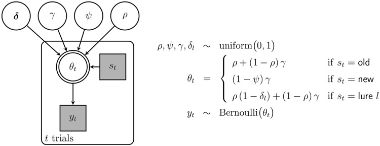
Figure 3 shows a graphical model representation of the MPT model for the old-new MST. In graphical models, nodes represent latent parameters and observed information, and specify how they are assumed to be related to one other. Children depend on their parents in the graph structure, and encompassing plates identify independent replications of the graph structure. Using the notation adopted by Lee & Wagenmakers (2013), the model parameters $\rho$, $\psi$, $\gamma$, and $\delta =({\delta }_1,\dots ,{\delta }_5)$ are shown as circular and unfilled nodes, because they represent continuous latent parameters. Whether the stimulus item on trial $t$ is an old, new, or level $l$ lure is represented by $s_t$. This node is square and shaded, because it represents discrete observed information. The model parameters and item information together determine the probability ${\theta }_t$ of an “old” response. This is shown as a double-bordered node because it is a deterministic function of the parameters and item information. Finally, the observed behavior on trial $t$ is $y_t=1$ if the response is “old” and $y_t=0$ if the response is “new”. This is discrete and observed, and depends on the response probability ${\theta }_t$. The trial-level information—the item information, response probability, and observed response—is encompassed by a plate that indicates the replication of this graph structure across trials.

Figure 3.

Graphical model representation of the MPT model for the old-new MST.

We implemented the graphical model in JAGS (Plummer, 2003), which is a high-level scripting language that automates fully Bayesian inference based on computational methods. Throughout this article, we generally sampled models using 8 independent chains with 1000 samples each after discarding 1000 burn-in samples. Convergence was assessed by visual inspection of traceplots and the standard $\widehat{R}$ statistic (Brooks & Gelman, 1997). JAGS scripts and MATLAB code for applying the models are provided in supplementary information.

Descriptive Adequacy

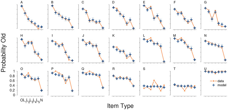
Figure 4 summarizes the descriptive adequacy (or “fit”) of the model to each participant. Each panel corresponds to a participant, and their behavior is shown by the orange line. The line follows the item ordering old $(\mathrm{O})$, level 1 lure $({\mathrm{L}}_1)$, level 2 lure $({\mathrm{L}}_2),\dots$, level 5 lure $({\mathrm{L}}_5)$, and new $(\mathrm{N})$. This ordering corresponds to decreasing similarity of the test item to a studied item. The line then indicates the proportion of “old” responses to each item type made by the participant. Optimal performance would be 100% “old” responses for old items and 0% “old” responses for all other items. The participants are labeled A–U and ordered in terms of decreasing overall accuracy across the panels. It is visually clear that more accurate participants show closer to optimal behavior, with lines that decrease as items become less similar.

Figure 4.

Descriptive adequacy of the MPT model for the old-new MST for all 21 participants.

The blue cross markers in Figure 4 show the mean of the posterior predictive distribution for the model and the lines above and below show the 95% credible interval. The posterior predictive distribution can be interpreted as the model’s attempt to re-describe the behavioral data. A descriptive adequate model should match the behavioral data. It is clear that the MPT model does this well for almost all of the participants. It closely matches the proportion of “old” responses to each item type, except for a couple of the worst-performed participants (e.g., Participants S and T). Most importantly, the model is able to capture the individual differences in participant behavior. For example, Participant A mostly responds “new” to the lure items, while Participant Q mostly responds “old”. The model is able to describe both of these extremes, and the intermediate sorts of behavior shown by the other participants.

Inferences

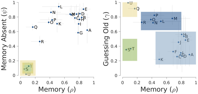
Figure 5 shows the parameter inferences made by the models. The left panel shows the relationship between the two memory parameters $\rho$ and $\psi$. The right panel shows the relationship between $\rho$ and the guessing old probability $\gamma$. Each participant’s joint posterior with respect to the pair of parameters is summarized by a marker for the posterior mean and error bars for 95% credible intervals for each marginal posterior. The two memory parameters are modestly correlated with each other, but are not identical. This is evidence in favor of the modeling assumption to distinguish between remembering that an item was studied versus remembering that an item was not studied. The memory and guessing old parameters appear to vary independently across participants, consistent with them measuring different memory and decision making processes.

Figure 5.

Parameter inferences of the MPT model for the old-new MST applied to the 21 participants.

Figure 5 superimposes colored squares that suggest a possible interpretation of the individual differences revealed by the parameter inferences. Each color corresponds to a potential interpretable subgroup. The yellow and green squares represent a different sort of contaminant behavior. In the left panel, it is clear that Participants S, T, and U in these subgroups have very low memory performance. In the right panel they are separated into Participants S and T who guess “old” and “new” about equally often, and Participant U (and potentially Q) who almost always respond “old”. Random responding and repeated responding are two common sorts of contaminant behavior (Zeigenfuse & Lee, 2010), and seem likely explanations for the poor performance of these participants. These interpretations are highly consistent with the observed behavior of Participants S, T, and U in Figure 4.

The right panel of Figure 5 identifies subgroups among participants who performed well in the task. The darker blue subgroup that includes Participants L, M, N, O, P, and R are inferred to have higher base-rates of guessing “old” and often have worse memory. The lighter blue subgroup includes the participants with the best memory and a lower probability of guessing “old”. This second subgroup generally corresponds to the participants with the greatest task accuracy.

Extension to Model Individual Differences

One way to incorporate the exploratory suggestion of subgroups into formal modeling is by extending the basic model to have hierarchical latent mixtures. As demonstrated by Bartlema et al. (2014, see also Lee 2018), hierarchical latent-mixture models provide a general statistical way of extending the cognitive models to account for two sorts of individual differences. The latent mixture extension allows for qualitatively different subgroups of participants, while the hierarchical extension allows for continuous variation within the subgroups. The latent mixture extension thus addresses both the contaminant behavior and the different types of attentive behavior. Intuitively, each component in the latent-mixture model corresponds to one of the colored boxes, and represents a different task strategy. The hierarchical extension then allows for variation in the parameters of participants within the same component, and represents fine-grained variability in exactly how a strategy is executed.

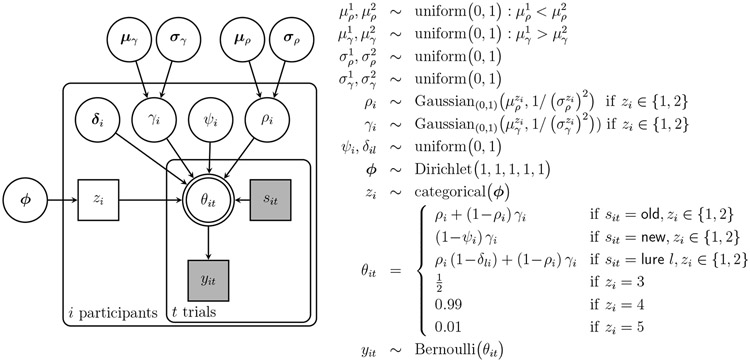
Figure 6 shows a graphical model that incorporates these extensions. There are five components in the latent-mixture model, indexed by a latent discrete parameter $z_i$ for the $i\text{th}$ participant. The first two components correspond to attentive responding and focus on individual differences in the memory ${\rho }_i$ and guessing base-rate ${\gamma }_i$ individual parameters. These parameters are assumed to be drawn from overarching truncated Gaussian distributions that are different depending on whether $z_i=1$ or $z_i=2$. In particular, the subgroup means are constrained to to be different with the first “low memory” subgroup having lower mean memory ${\mu }_{\rho }^1<{\mu }_{\rho }^2$ but greater base-rate of guessing “old” ${\mu }_{\gamma }^1>{\mu }_{\gamma }^2$ than the second “high memory” subgroup. Intuitively, this means $z_i=1$ corresponds to the dark blue strategy in Figure 5, in which worse memory for old items is compensated for by increasing guessing “old”, while $z_i=2$ corresponds to the light blue strategy in which old items are remembered better and the base-rate of guessing “old” is lower. The remaining three components correspond to different contaminant strategies, so that if $z_i=3$, there is always a 50-50 probability of responding “old” $(\theta =\frac{1}{2})$, if $z_i=4$ there is a high probability of responding “old” $(\theta =0.99)$, and if $z_i=5$ there is a high probability of responding “new” $(\theta =0.01)$.

Figure 6.

Graphical model representation of the MPT model for the old-new MST with a hierarchical latent-mixture extension to allow for individual differences.

The latent subgroup indicator is sampled for each participant from a categorical distribution $z_i\sim \text{categorical}(\varphi )$ so that $\varphi =({\varphi }_1,\dots ,{\varphi }_5)$ represents the base rate of each strategy. The base-rate itself is given a Dirichlet distribution $\varphi \sim \text{Dirichlet}(1,\dots ,1)$ which corresponds to the assumption that all possible base-rates are equally likely. The memory for absence ${\psi }_i$ and the discriminability probabilities ${\delta }_i$ do not define the proposed strategy differences and so continue to be allowed to vary independently across individuals.

Inferences

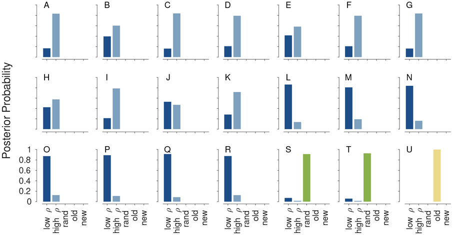
Figure 7 shows the inferences about subgroup membership, represented by the posterior distribution of $z_i$, made by the model for each participant. The subgroup inferences largely match the proposed groupings in Figure 5. The most accurate Participants A–K are inferred to belong to the “high memory” group, and less accurate Participants L–R are inferred to belong to the “low memory” group. The exception is Participant J, whose classification is uncertain. There is also significant uncertainty for Participant H. For the remainder of the participants the inferences about group membership are relatively confident, because the most likely subgroup has most of the posterior mass. The three participants anticipated to show contaminant behavior are inferred to belong to the appropriate “random” or “always respond old” subgroups.

Figure 7.

Subgroup inferences for each participant based on the hierarchical latent-mixture extension of the MPT model of the old-new MST.

While the subgroup inferences make sense, given the assumption of the different possible strategies, it is important to test for the evidence of these strategies as an account of individual differences. In particular, evidence for dividing the non-contaminant participants into two subgroups is important. (It could be argued that it is always useful to allow for the possibility of contaminant behavior, even if it is not observed in a specific data set). Evidence for two qualitatively different forms of task-attentive behavior is provided by the Bayes factor comparing a model that includes the subgroups to one that does not.

We approximated this Bayes factor using the posterior distribution of ${\varphi }_1$, which corresponds to the base-rate of “low memory” participants. If this base-rate is zero, the model reduces to having just one account of task-attentive behavior. Thus the Savage-Dickey method for estimating Bayes factors, which compares the ratio of prior to posterior densities at the point in parameter space where a more general model reduces to a nested special case, can be used (Wetzels et al., 2010). The Bayes factor is ${BF}_{10}=5$, meaning that the data are five times more likely under the model that incorporates the two subgroups. A figure showing the posterior distributions of the base-rate probabilities $\varphi$ is provided in the supplementary information.

Extension to Model Discriminability

The inferred discriminabilities ${\delta }_i=({\delta }_{i1},\dots ,{\delta }_{i5})$ measure the ability of the $i\text{th}$ person to discriminate a remembered study item from a current item on a test trial. In the modeling thus far, they are assumed to be independent. A stronger assumption would impose an order constraint, corresponding to the idea that more similar lures are more difficult to discriminate. Such an order constraint could be imposed in a strong way for each individual ${\delta }_{i1}<\dots <{\delta }_{i5}$, or in a weaker way in a hierarchically extended model by applying it to the mean of group distributions for each level of lure.

We pursue an alternative approach using a model of the relationship between similarity and discriminability. This is also a form of hierarchical extension, specifying additional modeling assumptions about the relationship in terms of parameters that can vary across individuals. In an exploratory way, we observed that the inferences about ${\delta }_i$ in the unconstrained model showed a mostly monotonic and often S-shaped (sigmoidal) pattern of increase in the probability of discrimination as lures become easier to distinguish. A figure showing these results is provided in the supplementary information.

On this basis, we propose the logistic model relating lure similarity to discrimination probability

$${\delta }_{il}=\frac{1}{1+\text{exp}\left\{-{\beta }_i\left(\frac{l}{n_l+1}-{\tau }_i\right)\right\}},$$ (7)

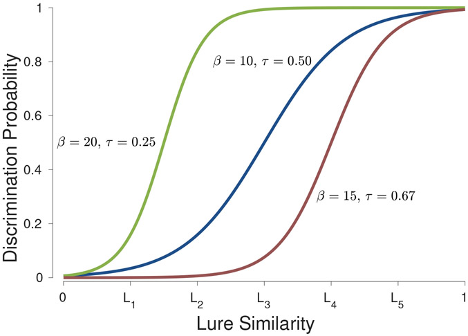
where $\tau$ can be interpreted as a threshold for discriminability and $\beta$ can be interpreted as a slope controlling how quickly discriminability increases. Figure 8 shows three specific examples of this relation that help understand the interpretation of the parameters. The lure similarity is normalized to lie between 0 and 1, so that the model is applicable to MST designs with any number of lure levels. The five levels for the current experiment have been mapped to normalized similarities of $1∕6,\dots ,5∕6$. This is achieved by the $\left(\frac{l}{n_l+1}-\tau \right)$ term in the shift of the logistic. Accordingly, smaller values of ${\tau }_i$ mean that the discriminability probability begins to increase for more difficult lures. The specific examples show that for ${\tau }_i=0.25$ there is already some probability of discriminating level 1 lures and discrimination is near perfect for level 2 lures. For ${\tau }_i=0.67$, in contrast, level 4 lures are discriminated about half the time and only the least similar level 5 lures are consistently discriminated. The specific examples also show how slopes ranging from ${\beta }_i=10$ to ${\beta }_i=20$ impact the rate of increase in discriminability.

Figure 8.

Modeled relationship between the similarity of a lure to a studied item and the probability of discriminating the lure.

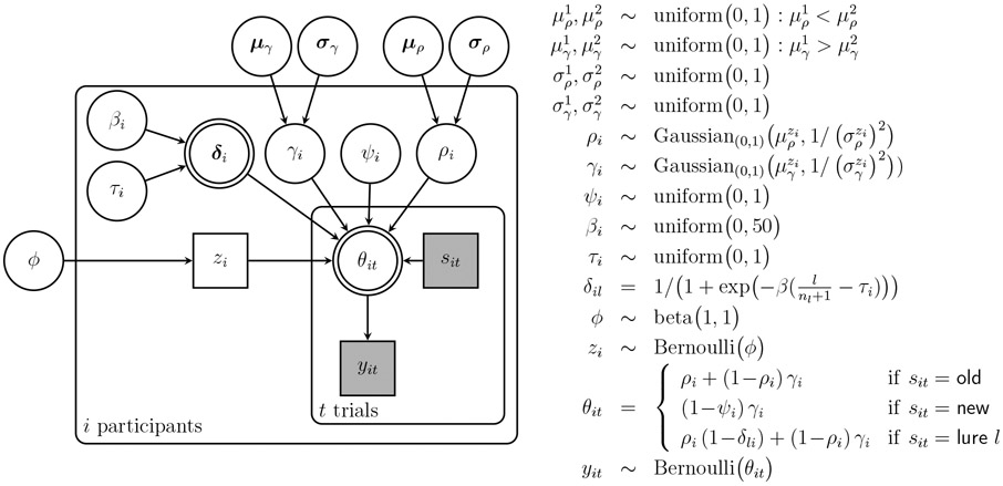
Figure 9 shows a graphical model that implements the hierarchical extension for discriminability. The key change is that ${\delta }_i$ now becomes a deterministic function of ${\beta }_i$ and ${\tau }_i$. In this model, only the latent-mixture components corresponding to attentive task behavior are included. Participants S, T, and U identified as contaminants by the analysis in Figure 7 are excluded from the analysis.

Figure 9.

Graphical model representation of the MPT model for the old-new MST with two subgroups of attentive participants and a logistic relationship between lure similarity and discriminability.

This model remains descriptively adequate using the same approach to posterior predictive analysis presented in Figure 4. This is an important finding, since the model has been significantly extended by introducing the two strategies, and significantly constrained by the logistic relationship between lure similarity and discriminability. A figure showing the posterior predictive analysis for this model is provided in the supplementary information.

Inferences

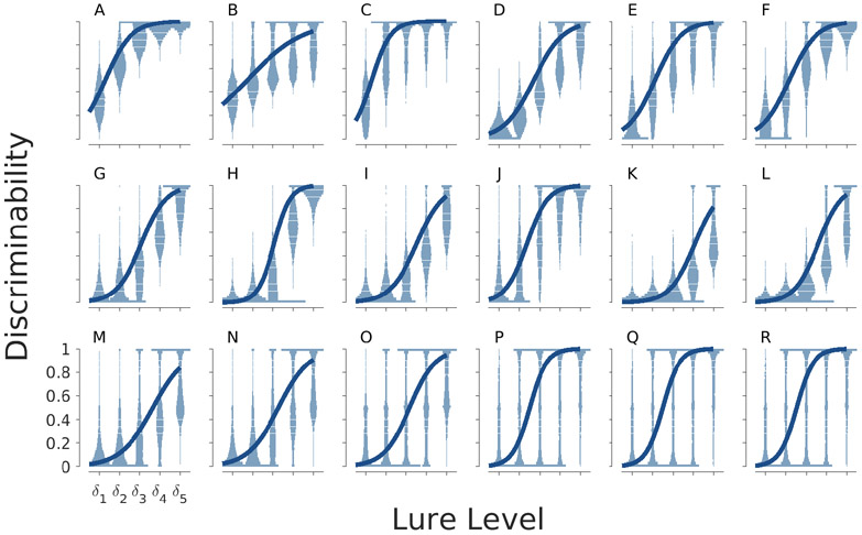
Figure 10 summarizes the inferences about the relationship between lure similarity and discriminability for each participant. The solid lines show the logistic function corresponding to the inferred posterior means of the slope ${\beta }_i$ and threshold ${\tau }_i$ for the $i\text{th}$ participant. The violin plots show the posterior distributions for each lure level. The slopes are reasonably similar: almost all of the participants have low discriminability for the most difficult level 1 lures, near perfect discriminability for the easiest level 5 lures, and a steady rate of increase between those extremes. There is much more variability in the thresholds at which the increase in discriminability begins. For example, Participants D and E begin to show increasing discriminability for the level 2 lures, Participants G and H begin to increase for the level 3 lures, and Participants K and L begin to increase for level 4 lures. The interpretable variability in the threshold ${\tau }_i$ suggests that it is a useful measure of lure discrimination. It can be interpreted as a measure of how similar or different lures need to be so that a participant has some ability to discriminate them from remembered studied items.

Figure 10.

The relationship between lure similarity and discriminability for each participant.

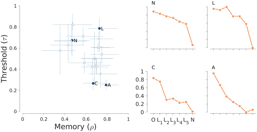
Figure 11 shows one way in which the model can be used to measure participants memory based on their MST performance. The left panel summarizes the joint posterior distribution of the memory $\rho$ and threshold $\tau$ parameters. Markers correspond to posterior means and error bars show 95% credible intervals. These two parameters capture the different aspects of memory assessed by the MST. The memory parameter corresponds to the ability to recall studied items. It essentially corresponds to the memory ability assessed by a standard recognition memory task. In support of this, the correlations of the posterior mean of $\rho$ with a standard frequentist $d^{\prime }$ measure of discriminability are $r=0.81$ between old and new items and $r=0.54$ between old and lure items. The threshold parameter, on the other hand, corresponds to the ability to discriminate remembered items from similar ones presented at test. It corresponds to the pattern separation capabilities that the MST aims to measure.

Figure 11.

Inferences about remembering probabilities and discriminability thresholds for all participants in the old-new MST (left panel), and summary behavior for four illustrative participants (right panels).

The results in Figure 11 show that these abilities vary largely independently across the participants. Memory recall probabilities can vary from about 40% to about 80% and thresholds can vary from about 20% to 80% across the normalized similarity scale. Four illustrative participants are highlighted in Figure 11 to emphasize the usefulness of this analysis. They approximately represent the four possibilities of low versus high memory and low versus high discriminability. The behavioral performances of these participants, as originally presented in Figure 4, are shown in the four right hand panels. Participants N and L are inferred to have worse discriminability than Participants C and A, which is evident behaviorally because they often respond “old” to lures. Participants N and C are inferred to have worse memory than Participants A and L, which is evident behaviorally because they fail to respond “old” to old stimuli more often.

MPT Model for the Old-Similar-New MST

Basic Model

We implemented the basic MPT model for the old-similar-new MST as a graphical model, following the same approach used to implement the old-new model in Figure 1. A figure showing the graphical model is provided in the supplementary information. The key change is that the behavioral data now take the form $y_t=1$ if the participant responded “old” on the $t\text{th}$ trial, $y_t=2$ if they responded “new”, and $y_t=3$ if they responded “similar”. In the same way, the trial information is extended to $s_t=1$ for old study items, $s_t=2$ for new items, and $s_t=3$ for lures. The choice probabilities ${\theta }_t$ are given by Equations 4, 5, and 6 for “old”, “new”, and “similar” responses.

Inferences

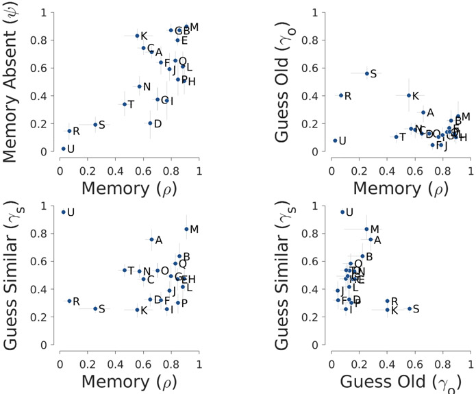
Figure 12 summarizes the inferences from applying this basic model to the old-similar-new MST data. There are two additional panels, showing the relationship between memory $\rho$ and the additional guessing similar ${\gamma }^s$ parameter, and between the guessing old ${\gamma }^o$ and guessing similar ${\gamma }^s$ parameters. Once again, there is a clear correlation between remembering an item was studied and remembering it was not studied. The analysis of memory and guessing parameters suggests that Participants R, S, and U may be contaminants. These three participants have much lower memory than the others. Participants R and S guess “old” more often than most other participants, perhaps to compensate for their poor memory. Participant U, on the other hand, appears to compensate by guessing “similar” with high probability. This suggests the need to consider an additional form of contaminant behavior based on repeatedly making “similar” responses.

Figure 12.

Inferences of basic old-similar-new MPT model, showing the relationship between the memory $\rho$, memory for absence $\psi$, guessing old ${\gamma }^o$, and guessing similar ${\gamma }^s$ parameters for the 21 participants.

Unlike the old-new analysis in Figure 5, there is no obvious subgroup structure for the memory and guessing behavior of the remaining attentive participants. They appear to form a single group with high memory probabilities, low probabilities of guessing “old” and moderate probabilities of guessing “similar”.

Extension to Model Individual Differences

We used the same modeling extensions and analyses as used for the old-new model. First, we developed a latent-mixture extension that allowed for two subgroups of attentive responding, defined in the same way as for the old-new model, and four possible types of contaminants: random responding, repeatedly responding “old”, repeatedly responding “new”, and repeatedly responding “similar”.

Inferences

A figure summarizing the inferences of this model, in the same form as Figure 7, is provided in the supplementary material. Participant R is inferred to be a random responding contaminant, and Participant U is inferred to be a repeated similar responding contaminant. Participant S is the only one inferred to belong to the low memory subgroup. The model comparison of the one vs two attentive subgroups, however, found some evidence in favor of a single group, with a Bayes factor of 2.3. A figure showing the posterior distributions for $\varphi$ is provided in the supplementary information.

While this model comparison does not provide conclusive evidence, it does favor the simpler account that there is only one qualitative form of attentive behavior in this version of the task. Accordingly, we considered a modified latent-mixture account, using only the mixture component for attentive behavior involving the model parameter, as the basis of subsequent modeling. Under this account, Participant S is inferred to be completing the task rather than being a contaminant.

Extension to Model Discriminability

Finally, we extended the model hierarchically to incorporate the same logistic relationship between lure similarity and discriminability used for the old-new model. Figures showing the inferred ${\delta }_{il}$ discriminabilities for each participant and lure both with and without this constraining model are provided in the supplementary information.

Descriptive Adequacy

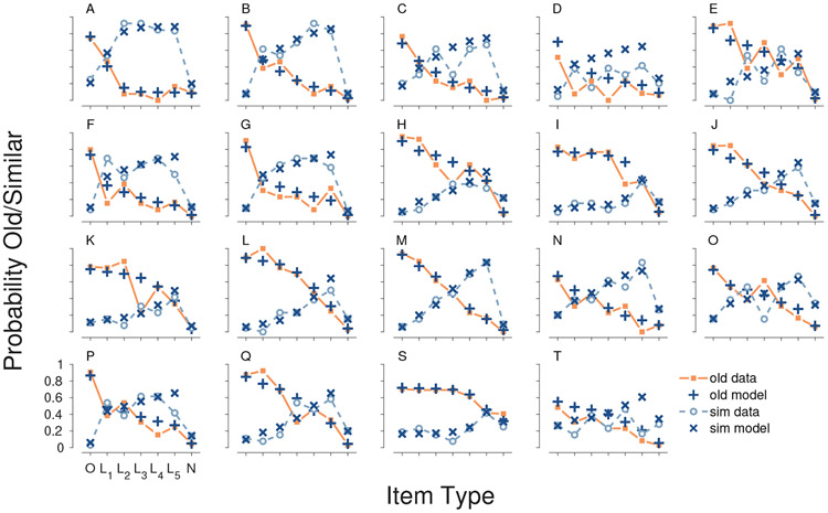
Figure 13 shows a posterior predictive analysis for checking the descriptive adequacy of this final model for the 19 non-contaminant participants. MST behavior is now summarized in terms of the probability of both “old” and “similar” responses for the different types of test items. These are shown by the solid orange and broken light-blue lines, respectively. The posterior predictive means are shown by plus and cross markers, respectively. There is generally excellent agreement for both types of responses for all of the participants.

Figure 13.

Descriptive adequacy of the extended MPT model for the old-similar-new MST for the 19 non-contaminant participants.

Inferences

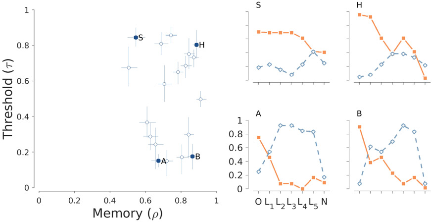
Figure 14 shows that the old-similar-new model also provides interpretable inferences about participants’ performance. The summary of the joint posterior distribution of memory $\rho$ and the discriminability threshold $\tau$ again shows they can vary largely independently across individuals. Four illustrative participants again highlight the usefulness of this analysis. Participants S and H are inferred to have worse discriminability than Participants A and B. This is evident behaviorally because S and H often respond “old” to lures whereas A and B often provide the correct “similar” response. Participants S and A are inferred to have worse memory than Participants H and B. This is evident behaviorally because they fail to respond “old” to old stimuli more often.

Figure 14.

Inferences about remembering probabilities and discriminability thresholds for all participants in the old-similar-new MST (left panel), and summary behavior for four illustrative participants (right panels).

The results in Figure 14 show that the old-similar-new model continues to provide the useful measurement demonstrated earlier for the old-new model. In particular, the memory parameter $\rho$ captures the ability to remember studied items, which is the key ability measured by recognition memory tasks. Conceptually, $\rho$ corresponds to what the recognition (REC) empirical measure is designed to measure. The REC is defined as the difference between the rate of “old” responses to old stimuli and the rate of “old” responses to new stimuli (Stark et al., 2013). The correlation between the posterior mean of $\rho$ and the REC measure for the non-contaminant participants is $r=0.90$. The discriminability threshold parameter $\tau$ captures the ability to distinguish between remembered and presented items that are similar, which is the key pattern separation capability measured by the introduction of lures to the MST. Conceptually, $\tau$ corresponds to what the lure discrimination index (LDI) is designed to measure. The LDI is defined as the difference between the rate of “similar” responses to lures and the rate of “similar” responses to new stimuli (Stark et al., 2013). The correlation between the posterior mean of $\tau$ and the LDI measure for the non-contaminant participants is $r=-0.83$.

Discussion

Model-based approaches to measuring people’s performance on diagnostic tasks have the ability to make inferences about latent psychological variables that cannot be directly measured. Models do this by formalizing and testing theoretical assumptions about task behavior and the structure of individual differences. In this article, we applied the model-based approach to the MST with the goal of measuring people’s ability to remember studied items, their ability to discriminate remembered items from presented lures, and their strategic guessing behavior when their memory fails. We developed novel MPT models of both the old-new and old-similar-new versions of the MST, showing that they were able to describe task performance at the individual level in a psychologically interpretable way, and identify meaningful subgroups of participants, including contaminant behavior.

In applying the models to data we relied exclusively on Bayesian methods. These methods have a number of important advantages. The most fundamental advantage is that they represent the uncertainty about inferences in a principled and complete way. The measurement of psychological variables will always involve uncertainty, because data are limited and noisy, and the models can only ever be useful approximations to true cognitive processes. Posterior distributions represent not just the most likely parameter values representing memory ability and decision making performance are, but how likely alternative values are. This representation of uncertainty allows the confidence in substantive conclusions to be calibrated appropriately.

The sequence of models we developed highlights another important advantage of Bayesian methods, which is the flexibility to build more complete accounts of task performance and individual difference (Bartlema et al., 2014; Lee, 2018). We used hierarchical latent-mixture modeling to account for both qualitative and quantitative patterns of individual differences in the old-new task, and a different sort of hierarchical extension to model the relationship between lure similarity and discriminability. Bayesian methods, through Bayes factors and posterior predictive checks, allowed these extended models to be justified in terms of the behavioral data. The end results of the exploratory modeling process were MPT models for both tasks that characterized individual memory in terms of two key parameters: the probability of remembering items $\rho$ and the ability to discriminate remembered items from lures $\tau$.

Beyond the meaningful measurement of individuals and groups, the model-based approach provides new insights into the merits of tasks themselves. For the experimental data we considered, the old-similar-new task has the advantage of providing a simpler modeling account of individual differences. It did not require considering two subgroups of attentive behavior. It is possible this is a general advantage, since the presence of subgroups for the old-new task emerges from different strategies participants use when they are unable to remember and discriminate. The lack of a “similar” response option potentially is the basis for these different strategies. When only “old” and “new” responses are available, participants have to decide what level of perceived agreement is low enough to warrant a “new” response even though there is some strength of remembrance. Only responding “old” when they are certain of a match leads to different behavior than only responding “new” when they are certain of no match leads to different responses, even for two participants with the same underlying memory properties. The availability of a “similar” response does not eliminate the need for decision strategies, but it does lessen their impact. At least for the current data, this made modeling significantly simpler.

A different perspective on the relationship between tasks is not to treat comparison as a competition to reveal the best task, but to treat them as at least partly complementary ways of measuring cognitive capabilities. As emphasized above, an advantage of model-based approaches using Bayesian methods is that they can extend to capture task nuances. Combining behavior on both the old-new and old-similar-new tasks to improve individual measurement is a promising direction for future research. In the within-participants data we used, the product-moment correlation of the posterior expectations across participants between the two tasks is $r=0.45$ for $\rho$ and $r=0.53$ for $\tau$. Understanding what these correlations mean is a challenging question, because there are many (not mutually exclusive) possibilities. The lack of perfect correlation could arise from limitations in one or both tasks controlling what can be measured, or because the cognitive models are too simple and miss important characteristics of the underlying memory and decision processes, or because the underlying cognitive properties generating task behavior are not stable. The model-based approach to exploring these possibilities is to develop a joint or common-cause model that attempts to account for behavior on both tasks simultaneously (Lee, 2018; Turner et al., 2013). For example, latent-trait joint models provides a more complete way to assess the relationships between parameters (Klauer, 2010), and complete common-cause models can test possibilities such as memory components of the model being consistent across tasks but decision processes changing to adapt to different task demands.

In its traditional frequentist form, the LDI measure from the MST is correlated with age-related cognitive decline, with various MRI measures of hippocampal function and connectivity, and has been used in clinical populations such as dementia, schizophrenia, and depression (see Stark et al., 2019, for a review). It has proven effective in various clinical trials including A4, tracking odds of clinical decline towards Alzheimer’s (Jutten et al., 2021; Papp et al., 2021) and HOPE4MCI, showing drug treatment effects (Bakker et al., 2015). Here, $\rho$ and $\tau$ correlate well with REC and LDI and are meant to reflect similar concepts. However, the potential advantage of the model-based $\rho$ measure is that it directly measures the latent process of remembering and does not consider “old” responses caused by guessing. In the same way, the potential advantage of $\tau$ is that is describes how a latent discrimination process changes with item similarity, in the situation where the item has been remembered, and is unaffected by guessing. This more direct measurement may make $\rho$ and $\tau$ more sensitive measures of memory performance than empirical measures like REC and LDI. Examining whether the mode developed here captures these established effects better is an important direction for future research.

References

- Alexander GE, Satalich TA, Shankle WR, & Batchelder WH (2016). A cognitive psychometric model for the psychodiagnostic assessment of memory-related deficits. Psychological Assessment, 28(3), 279–293, 10.1037/pas0000163. [DOI] [PubMed] [Google Scholar]
- Bakker A, Albert MS, Krauss G, Speck CL, & Gallagher M (2015). Response of the medial temporal lobe network in amnestic mild cognitive impairment to therapeutic intervention assessed by fMRI and memory task performance. NeuroImage: Clinical, 7, 688–698, 10.1016/j.nicl.2015.02.009. [DOI] [PMC free article] [PubMed] [Google Scholar]
- Bartlema A, Lee MD, Wetzels R, & Vanpaemel W (2014). A Bayesian hierarchical mixture approach to individual differences: Case studies in selective attention and representation in category learning. Journal of Mathematical Psychology, 59, 132–150, 10.1016/j.jmp.2013.12.002. [DOI] [Google Scholar]
- Batchelder WH & Riefer DM (1980). Separation of storage and retrieval factors in free recall of clusterable pairs. Psychological Review, 87(4), 375–397, 10.1037/0033-295x.87.4.375. [DOI] [Google Scholar]
- Brooks SP & Gelman A (1997). General methods for monitoring convergence of iterative simulations. Journal of Computational and Graphical Statistics, 7, 434–455, 10.2307/1390675. [DOI] [Google Scholar]
- Chan AS, Salmon DP, & De La Pena J (2001). Abnormal semantic network for “animals” but not “tools” in patients with Alzheimer’s disease. Cortex, 37, 197–217, 10.1016/S0010-9452(08)70568-9. [DOI] [PubMed] [Google Scholar]
- De Leeuw JR (2015). jsPsych:A JavaScript library for creating behavioral experiments in a web browser. Behavior Research Methods, 47(1), 1–12, 10.3758/s13428-014-0458-y. [DOI] [PubMed] [Google Scholar]
- De Leeuw JR & Motz BA (2016). Psychophysics in a web browser? Comparing response times collected with JavaScript and Psychophysics Toolbox in a visual search task. Behavior Research Methods, 48(1), 1–12, 10.3758/s13428-015-0567-2. [DOI] [PubMed] [Google Scholar]
- Erdfelder E, Auer T-S, Hilbig BE, Aßfalg A, Moshagen M, & Nadarevic L (2009). Multinomial processing tree models: A review of the literature. Zeitschrift für Psychologie/Journal of Psychology, 217(3), 108–124, 10.1027/0044-3409.217.3.108. [DOI] [Google Scholar]
- Green DM & Swets JA (1966). Signal Detection Theory and Psychophysics. New York: Wiley. [Google Scholar]
- Hilbig BE (2016). Reaction time effects in lab-versus Web-based research: Experimental evidence. Behavior Research Methods, 48(4), 1718–1724, https://doi.org/doi: 10.3758/s13428-015-0678-9. [DOI] [PubMed] [Google Scholar]
- Jutten RJ, et al. (2021). Monthly at-home computerized cognitive testing to detect diminished practice effects in preclinical Alzheimer’s disease. Frontiers in Aging Neuroscience, 13, 10.3389/fnagi.2021.800126. [DOI] [PMC free article] [PubMed] [Google Scholar]
- Kellen D & Klauer KC (2014). Discrete-state and continuous models of recognition memory: Testing core properties under minimal assumptions. Journal of Experimental Psychology: Learning, Memory, and Cognition, 40(6), 1795–1804, 10.1037/xlm0000016. [DOI] [PubMed] [Google Scholar]
- Klauer KC (2010). Hierarchical multinomial processing tree models: A latent-trait approach. Psychometrika, 75, 70–98, 10.1007/s11336-009-9141-0. [DOI] [Google Scholar]
- Klauer KC & Kellen D (2018). RT-MPTs: Process models for response-time distributions based on multinomial processing trees with applications to recognition memory. Journal of Mathematical Psychology, 82, 111–130, 10.1016/j.jmp.2017.12.003. [DOI] [Google Scholar]
- Lacy JW, Yassa MA, Stark SM, Muftuler LT, & Stark CE (2011). Distinct pattern separation related transfer functions in human CA3/dentate and CA1 revealed using high-resolution fMRI and variable mnemonic similarity. Learning & Memory, 18, 15–18, 10.1101/lm.1971111. [DOI] [PMC free article] [PubMed] [Google Scholar]
- Lange K, Kühn S, & Filevich E (2015). “Just Another Tool for Online Studies”(JATOS): An easy solution for setup and management of web servers supporting online studies. PloS one, 10, e0130834, 10.1371/journal.pone.0130834. [DOI] [PMC free article] [PubMed] [Google Scholar]
- Lee MD (2018). Bayesian methods in cognitive modeling. In Wixted J & Wagenmakers E-J (Eds.), The Stevens’ Handbook of Experimental Psychology and Cognitive Neuroscience. Volume 5: Methodology chapter 2, (pp. 37–84). John Wiley & Sons, fourth edition. [Google Scholar]
- Lee MD, Bock JR, Cushman I, & Shankle WR (2020). An application of multinomial processing tree models and Bayesian methods to understanding memory impairment. Journal of Mathematical Psychology, 95, 102328, 10.1016/j.jmp.2020.102328. [DOI] [Google Scholar]
- Lee MD & Wagenmakers E-J (2013). Bayesian Cognitive Modeling: A Practical Course. Cambridge University Press. [Google Scholar]
- MacMillan N & Creelman CD (2004). Detection Theory: A User’s Guide (2nd ed.). Hillsdale, NJ: Erlbaum. [Google Scholar]
- Papp KV, et al. (2021). The Computerized Cognitive Composite (C3) in an Alzheimer’s disease secondary prevention trial. The Journal of Prevention of Alzheimer’s Disease, 8(1), 59–67, 10.14283/jpad.2020.38. [DOI] [PMC free article] [PubMed] [Google Scholar]
- Pinet S, Zielinski C, Mathôt S, Dufau S, Alario F-X, & Longcamp M (2017). Measuring sequences of keystrokes with jsPsych: Reliability of response times and interkeystroke intervals. Behavior Research Methods, 49(3), 1163–1176, 10.3758/s13428-016-0776-3. [DOI] [PubMed] [Google Scholar]
- Plummer M. (2003). JAGS: A program for analysis of Bayesian graphical models using Gibbs sampling. In Hornik K, Leisch F, & Zeileis A (Eds.), Proceedings of the 3rd International Workshop on Distributed Statistical Computing (DSC 2003). [Google Scholar]
- Snodgrass JG & Corwin J (1988). Pragmatics of measuring recognition memory: Applications to dementia and amnesia. Journal of Experimental Psychology: General, 117(1), 34–50, 10.1037/0096-3445.117.1.34. [DOI] [PubMed] [Google Scholar]
- Stark CE, Clemenson GD, Aluru U, Hatamian N, & Stark SM (2021). Playing Minecraft improves hippocampal-associated memory for details in middle aged adults. Frontiers in Sports and Active Living, 3, 685286, 10.3389/fspor.2021.685286. [DOI] [PMC free article] [PubMed] [Google Scholar]
- Stark SM, Kirwan CB, & Stark CE (2019). Mnemonic Similarity Task: A tool for assessing hippocampal integrity. Trends in Cognitive Sciences, 23(11), 938–951, 10.1016/j.tics.2019.08.003. [DOI] [PMC free article] [PubMed] [Google Scholar]
- Stark SM, Stevenson R, Wu C, Rutledge S, & Stark CE (2015). Stability of age-related deficits in the mnemonic similarity task across task variations. Behavioral Neuroscience, 129(3), 257–268, 10.1037/bne0000055. [DOI] [PMC free article] [PubMed] [Google Scholar]
- Stark SM, Yassa MA, Lacy JW, & Stark CE (2013). A task to assess behavioral pattern separation (BPS) in humans: Data from healthy aging and mild cognitive impairment. Neuropsychologia, 51, 2442–2449, 10.1016/j.neuropsychologia.2012.12.014. [DOI] [PMC free article] [PubMed] [Google Scholar]
- Turner BM, Forstmann BU, Wagenmakers E-J, Brown SD, Sederberg PB, & Steyvers M (2013). A Bayesian framework for simultaneously modeling neural and behavioral data. NeuroImage, 72, 193–206, 10.1016/j.neuroimage.2013.01.048. [DOI] [PMC free article] [PubMed] [Google Scholar]
- Villarreal M, Stark CE, & Lee MD (2022). Adaptive design optimization for a Mnemonic Similarity Task. Journal of Mathematical Psychology, 108, 102665, 10.1016/j.jmp.2022.102665. [DOI] [PMC free article] [PubMed] [Google Scholar]
- Westfall HA & Lee MD (2021). A model-based analysis of the impairment of semantic memory. Psychonomic Bulletin & Review, 28(5), 1484–1494, 10.3758/s13423-020-01875-9. [DOI] [PubMed] [Google Scholar]
- Wetzels R, Grasman RPPP, & Wagenmakers E (2010). An encompassing prior generalization of the Savage-Dickey density ratio test. Computational Statistics and Data Analysis, 54, 2094–2102. [Google Scholar]
- Yassa MA, Lacy JW, Stark SM, Albert MS, Gallagher M, & Stark CE (2011). Pattern separation deficits associated with increased hippocampal CA3 and dentate gyrus activity in nondemented older adults. Hippocampus, 21(9), 968–979, 10.1002/hipo.20808. [DOI] [PMC free article] [PubMed] [Google Scholar]
- Zeigenfuse MD & Lee MD (2010). A general latent assignment approach for modeling psychological contaminants. Journal of Mathematical Psychology, 54(4), 352–362, 10.1016/j.jmp.2010.04.001. [DOI] [Google Scholar]