Time-Resolved Fluorescence Anisotropy from Single Molecules for Characterizing Local Flexibility in Biomolecules

Abstract

We describe a protocol for conducting time-resolved fluorescence anisotropy at the single-molecule level using confocal microscopy to investigate the local flexibility and dynamics of the deoxyribonucleic acid (DNA)-binding forkhead (FKH) domain of the FoxP1 transcription factor. FoxP1 dimerizes through a three-dimensional domain-swapping (3D-DS) mechanism, forming a disordered intermediate with or without DNA. Since 3D-DS involves an intrinsically disordered region, understanding its behavior is crucial for elucidating the structural and functional properties of FoxP1. Using a single-cysteine-labeled FoxP1, we conducted single-molecule fluorescence anisotropy (smFA) experiments, applying dynamic anisotropy Photon Distribution Analysis (daPDA) and time-resolved anisotropy Burst Variance Analysis (traBVA) approaches to probe local flexibility and dynamics. This protocol provides a detailed, step-by-step guide for smFA measurements, emphasizing time-resolved analyses, variance, and probability distribution techniques to capture structural dynamics across different timescales. This approach enabled us to relate dynamics and heterogeneity to FoxP1 dimerization and DNA binding, highlighting the complex action mechanism that characterizes this transcription factor.

Introduction

The functional activity of biomolecules depends on their molecular flexibility and structural dynamics^1,2,3. Naturally, biomolecules experience constant thermal fluctuations, ranging from rapid movements to long-term conformational changes influencing their function (Figure 1)⁴. In biomolecules, local backbone motions contribute to larger-scale global movements, including hinge bending in enzymes and significant conformational changes in motor proteins. Structure determination methods such as nuclear magnetic resonance (NMR)⁵, X-ray crystallography⁶, and cryogenic electron microscopy (cryo-EM)⁷ have revealed multiple conformations in various biomolecules. Nevertheless, connecting the local fluctuations to large conformational dynamics of biomolecules and their role in function are mostly unexplored. Relating dynamics and structure can be challenging, especially for intrinsically disordered proteins (IDPs)^8,9,10. Unlike structured proteins, IDPs do not maintain a stable tertiary structure. Instead, they undergo extensive conformational changes with similar free energy levels, enabling a wide range of biological activities^11,12.

Figure 1: Dynamic range of biomolecules and fluorescence anisotropy methods.

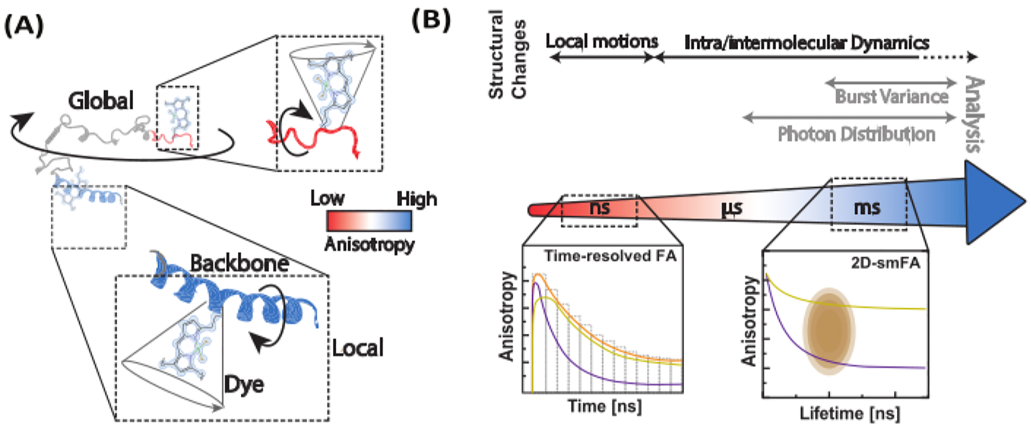
(A) The anisotropy of small fluorophores tethered to various positions along the backbone of the biomolecule of interest informs local structural dynamics. (B) Timescales probed by fluorescence intensity decays (time-resolved fluorescence anisotropy, FA) and single-molecule histograms of confocal single-molecule microscope data.

Several experimental approaches have been employed to investigate the conformational dynamics of proteins by probing their molecular flexibility^{1,13,14,15,16}. Among these, NMR stands out for its ability to provide atomic-level resolution across various timescales, from tens of picoseconds to several hours¹². However, determining macromolecular flexibility remains challenging due to the high degrees of freedom and for large-size proteins; thus, NMR is often limited to studying biomolecules of around 100 kDa¹⁷.

Given the structural complexity of highly dynamic proteins like IDPs, additional methodological advancements have been developed to explore local and long-range conformational space to understand their function¹¹. Single-molecule multiparameter Fluorescence Spectroscopy (smMFS)^{18,19,20,21,22} offers extensive information on biomolecules, providing crucial insights into their function, conformational dynamics, binding states, and stoichiometry. However, interpreting the vast amount of structural data obtained from biomolecules is challenging, and factors such as molecular dynamics, fluorophore behavior, and the complex behavior of molecules can further complicate data analysis^{23,24,25,26,27,28}.

We employ single-molecule fluorescence anisotropy (smFA) as a robust method for assessing local and global dynamics along the backbone of biomolecules (Figure 1A). Fluorescence anisotropy, first described by Perrin²⁹ and introduced by Weber^30,31 as a bioanalytical tool³², was later adapted for single-molecule studies with the advent of time-resolved fluorescence techniques and the increment of detectors’ sensitivity^{33,34,35,36,37}. smFA spans a broad range of timescales -- from picoseconds to several hours -- and complements the data obtained from single-molecule Förster Resonance Energy Transfer (smFRET) experiments³⁸.

smFA can be visualized in various formats to extract critical information about biomolecular dynamics (Figure 1B). Time-resolved fluorescence anisotropy decays are one-dimensional histograms that capture dynamics on the picosecond to nanosecond timescale^39,40. Two-dimensional single-molecule histograms, which correlate fluorescence lifetime with anisotropy for individual molecules, can reveal anisotropy state heterogeneity and provide visual insights into potential dynamics within the observation time in confocal experiments (~ms)^41,42. For studying sub-millisecond dynamics, dynamic anisotropy photon distribution analysis (daPDA) can be used, while time-resolved anisotropy Burst Variance Analysis (traBVA) offers a robust method for confirming specific dynamics around milliseconds⁴³ (Figure 1B).

These methods complement more traditional tools, such as polarization-resolved fluorescence correlation spectroscopy (pFCS), which has a broader spectrum^44,45,46,47. Overall, multiple data analysis tools for smFA facilitate identifying local and global conformational changes, provided proper calibration is considered.

Here, we apply smFA to study the DNA binding of the human FoxP1 transcription factor^48,49,50,51. This protein adopts domain-swapped dimer due to the intrinsically disordered nature of its polypeptide chain, which is notably affected depending on the quaternary state of the protein and the presence of DNA. We generated different single-cysteine mutants to label with BODIPY-FL, performed smFA experiments, and employed daPDA and trBVAa. This approach allowed us to relate dynamics and heterogeneity to FoxP1 dimerization and the DNA binding, highlighting the complex mechanism of action that characterizes this transcription factor.

Protocol

NOTE: Selecting the proper fluorophore is essential for smFA experiments. Biomolecules can be labeled at site-specific positions either by modifying amino acids in proteins or nucleotide bases in nucleic acids with fluorescent markers, depending on the available reactive groups. Among organic dyes⁵², the Alexa Fluor, Cy, BODIPY, and Janelia Farms families are the most popular choices for smFA, thanks to their long fluorescence lifetimes, photostability, and high quantum yields. BODIPY-FL is often favored for its extended fluorescence lifetime, superior quantum yield, and short connecting linker. Additionally, alternative fluorophores are commonly used in drug screening where bulk techniques are preferred⁵³. Chimeric fluorescent proteins can also be used for live-cell anisotropy experiments and imaging, although there is a limitation of a lower dynamic range.

1. Buffer preparation

NOTE: Wear gloves, eye protection goggles, and a laboratory coat while doing laboratory experiments.

1. Standard buffer (20 mM 4- (2-hydroxyethyl)-1-piperazineethanesulfonic acid [HEPES], pH 7.8, 150 mM NaCl): Dissolve 2.38 g of HEPES, 4.38 g of NaCl in 400 mL of ultra-pure water, adjust pH to 7.8 and make the final volume to 500 mL.

2. Lysis buffer (20 mM HEPES, pH 7.8, 150 mM NaCl, 0.1 mM phenylmethylsulfonyl fluoride [PMSF], 10 μg/mL DNAse): Dissolve 2.38 g of HEPES, 4.38 g of NaCl, and 8.71 mg of PMSF and a final concentration of 10 μg/mL DNAse in 400 mL of ultra-pure water, adjust pH to 7.8 and make the final volume to 500 mL.

3. Equilibration buffer (50 mM phosphate buffered saline [PBS], 150 mM NaCl, and 10 mM Imidazole; pH 7.4): Dissolve 5.05 g of Na₂HPO₄, 0.85 g of NaH₂PO₄, 4.38 g of NaCl and 0.34 g of Imidazole in 400 mL of ultra-pure water, adjust pH to 7.4 and make the final volume to 500 mL.

4. Wash buffer (50 mM PBS, 150 mM NaCl, and 30 mM Imidazole; pH 7.4): Dissolve 5.05 g of Na₂HPO₄, 0.85 g of NaH₂PO₄, 4.38 g of NaCl and 1.02 g of Imidazole in 400 mL of ultra-pure water, adjust pH to 7.4 and make the final volume to 500 mL.

5. Elution buffer (50 mM PBS, 150 mM NaCl, and 250 mM Imidazole; pH 7.4): Dissolve 5.05 g of Na₂HPO₄, 0.85 g of NaH₂PO₄, 4.38 g of NaCl and 8.5 g of Imidazole in 400 mL of ultra-pure water, adjust pH to 7.4 and make the final volume to 500 mL.

6. PBS buffer (50 mM Sodium Phosphate Buffered Saline, 150 mM NaCl, pH 7.4). Dissolve 5.05 g of Na₂HPO₄, 0.85 g of NaH₂PO₄, and 4.38 g of NaCl in 400 mL of ultra-pure water, adjust pH to 7.4, and make the final volume to 500 mL.

7. Sterilize all buffers by filtering the solution using 0.22 μm pore size filters and store the buffers at room temperature (RT).

8. Filter the standard buffer using a charcoal filter for single-molecule acquisition.

2. Fluorescent probes

1. BODIPY-FL: Dissolve 5 mg vial containing BODIPY-FL by adding a final volume of 1.29 mL of freshly opened dimethyl sulfoxide (DMSO) to get the final concentration of 10 mM BODIPY-FL.

2. Rhodamine 110: Dissolve 3.67 mg of Rhodamine 110 by adding a final volume of 1 mL of freshly opened DMSO to get the final concentration of 10 mM Rhodamine 110.

   NOTE: Fluorescent probes need to be avoided when exposed to light. Always use a light-sensitive tube (amber color) and wrap it with aluminum foil. If DMSO is already opened, it must be kept in the desiccator to increase its shelf life.

3. Prepare small-volume aliquots of the prepared fluorescent probe and store it at −20 °C until further use.

   NOTE: Avoid freeze-thaw cycles to improve its labeling efficiency.

3. Calibration measurements

1. Perform multiparameter fluorescence detection (MFD) experiments on a home-built polarization resolved setup with 4 detection channels and 2 pulsed lasers (blue 485 nm and red 640 nm)⁵⁴. However, for anisotropy measurements, use the blue laser and two detector channels.

2. Turn on the detector channels (parallel and perpendicular) and the blue laser power.

3. Make sure the laser power is set to 60 μW and open the time-correlated single photon counting (TCSPC) software³⁶ control panel.

4. Mix 1 μL of 100 nM Rhodamine 110 and 49 μL of distilled water to make a final concentration of 2 nM Rhodamine 110. Add 50 μL of 2 nM Rhodamine 110 to the center of the cover glass for calibration measurements.

5. Next, add a drop of immersion liquid (either oil or water, but taking care about sharing the same refractive index) on top of the microscope objective lens to increase the resolving power of the microscope.

6. Place the cover glass on top of the objective lens and make sure the water droplet is at the center of the microscope objective.

7. Adjust the image plane to be inside the solution and above the glass surface.

8. Adjust the knob to find the second bright focal point and turn to one and a half points. Focus the laser at the interface of the glass and liquid.

9. Maximize the number of photons detected by adjusting the pinhole position (70 μm) while monitoring the photon count rate.

10. Open the software in the time-tagged time-resolved (TTTR, or T3) mode panel and click the Start button. Record the count rate for 120 s and save the Rhodamine 110.ptu file format using the acquisition software. This acquisition time should be enough considering the concentration (2 nM).

11. For background measurements, add 50 μL of distilled water to the center of the cover glass and repeat the steps 3.5–3.10. However, record the photon count rate for 300 s and save the water.ptu file.

12. For other background measurements, add 50 μL of standard buffer to the center of the cover glass and repeat steps 3.5–3.10. Record the photon count rate for 300 s and save standard buffer.ptu file. Then, analyze the data using burst integration fluorescence lifetime (BIFL) analysis software.

4. Calibration and data analysis

1. Open the BIFL software and click on confirm the setup from the automatic window. Next, click on get parameters from file, then OK.

2. For the measurement to analyze, click on data path array and select it.

3. Next, load the water measurement water.ptu file for arrays such as Green scatter. Similarly, select the standard buffer.ptu file for Green background. For Green thick, select Rhodamine 110.ptu.

4. Under the single molecule selection parameters, click Next, and then Adjust to display a new pop-up window. Click threshold to change the inter-photon arrival time and select single-molecule event time for the mean inter-photon arrival time (dt). Next, click min. # to select the minimum number of photons per single molecule event, then close the pop-up window by clicking Return. Then, click OK.

5. Next, click Color fit parameters to adjust the initial fluorescence lifetime for Green, colors that are generated with fluorescence decay parameters. Adjust Prompt and Delay values by modifying From and To values. Then close the pop-up window by clicking Return. Then, click OK.

6. Click Save to process the ASCII files and save them in a selected folder. Then, process the data for time-resolved fluorescence anisotropy decay using ChiSurf²², Photon Distribution Analysis^55,56, or Burst Variance Analysis^57,58.

   NOTE: Exemplary data and step-by-step descriptions on how to use ChiSurf, PDA, and BVA are available at github.com/Fluorescence-Tools/chisurf, github.com/Fluorescence-Tools/tttrlib, www.mpc.hhu.de/en/software/mfd-fcs-and-mfis and github.com/SMB-Lab/feda_tools, respectively. The experimental data is available at Zenodo (10.5281/zenodo.13371503).

5. FoxP1 protein preparation

1. Recombinant FoxP1 bacterial overexpression

   1. Perform transformation into E. coli C41 bacterial cells after quick-change site-directed polymerase chain reaction (PCR) mutagenesis.
   2. Prepare LB media and autoclave to sterilize it.
   3. Pre-inoculate a single E. coli C41 colony by adding into 5 mL of LB medium containing 5 μL (100 μg/mL) ampicillin. Let incubate at 37 °C overnight on an incubator shaker.
   4. Next day, inoculate large-scale bacterial culture by adding overnight pre-inoculum into 500 mL of LB media with pre-added antibiotic with a ratio of 1:500.
   5. Monitor the growth of the culture by measuring the absorbance of the culture at 600 nm.
   6. When the optical density reaches between ~0.5–0.7, induce the protein expression by adding a final concentration of 0.5 mM isopropyl-β-d-1-thiogalactopyranoside (IPTG) and keep the culture at 15 °C on an incubator shaker overnight.
   7. After achieving an optical density (600 nm) in the range of 1.4–1.6, harvest the bacterial cells by centrifugation at 3000 g for 20 min at 4 °C. Discard the supernatant and store the pellet at −20 °C until use.
2. Recombinant FoxP1 purification

   1. Lyse E. coli C41 cells by adding lysis buffer using any lysis methods such as sonication, liquid homogenization, French press, etc.
   2. Centrifuge the lysate at 14000 g for 10 min at 4 °C.
   3. For His₆-tagged proteins, wash the Ni²⁺-NTA affinity column and equilibrate with NiSO₄ using fast protein liquid chromatography (FPLC).
   4. Load the His₆-tagged FoxP1 protein into the equilibrated Ni²⁺-NTA affinity column.
   5. Elute the FoxP1 protein from the Ni²⁺-NTA column using a linear gradient of the elution buffer.
   6. After the protein is eluted, perform dialysis for buffer exchange. Add protein into an equilibration buffer without Imidazole and dialyze overnight using a magnetic stirrer at 4 °C.
      NOTE: If the protein is purified using a different method, do the buffer exchange accordingly.
   7. To remove the His₆-tag, add tobacco etch virus (TEV) protease (1:100 ratio of TEV:FoxP1) to the dialysis overnight.
      NOTE: His₆-tag digestion can also be performed by adding on-column TEV protease digestion. This step would improve the yield of the protein of interest.
   8. Next day, repeat the steps from 5.2.3–5.2.5. However, this time, elute the protein in the wash buffer rather than the elution buffer.
   9. Concentrate the protein to an appropriate volume by adding PBS buffer and quantify the protein using absorbance at 280 nm, considering the extinction coefficient of the protein.
3. Recombinant FoxP1 labeling

   1. Incubate 50–100 μM FoxP1 protein with a 10-fold molar excess of either Dithiothreitol (DTT) or tris (2-carboxyethyl)phosphine (TCEP) with a final volume of 500 μL at RT for 30 min.
   2. Perform buffer exchange using PD 10 desalting columns. Place the PD10 column into a 50 mL centrifuge tube using a column adapter.
   3. Equilibrate the PD10 column by adding 5 mL of PBS buffer and centrifuge at $1000\times g$ for 2 min. Repeat this step 3 times.
   4. Keep the PD10 column in a fresh 50 mL tube and add 2 mL of PBS buffer into the column. Then, add 500 μL of FoxP1 protein from step 1 into the column. Elute the protein bycentrifuging $1000\times g$ for 2 min and collect the protein.
   5. Concentrate the protein by adding it into ultra centrifugal filters (10 kDa MWCO), centrifuge at $7500\times g$ for 10 min, and collect the elute.
   6. Measure the protein concentration, add BODIPY with 30% equivalent of cysteine concentration in the protein, and place it on a rotator for 2 h at 4 °C.
   7. Perform buffer exchange and concentrate the protein as discussed in steps 5.3.2–5.3.5.
   8. Check the protein concentration using a spectrophotometer or a colorimetric assay, such as the Bradford or Lowry method, and the concentration of the dye by absorbance at 500 nm.
   9. Measure the degree of labeling using the following formula:
      (${\text{A}}_{\text{Dye}}/{\epsilon }_{\text{Dye}}$)/(molecular weight of protein/milligram of protein per milliliter) = moles of dye/moles of protein Where ${\text{A}}_{\text{Dye}}$ and ${\epsilon }_{\text{Dye}}$ are the absorbance value of the dye and the molar extinction coefficient of the dye at the maximum absorbance wavelength, respectively⁵⁹. When measured at 280 nm, the real absorbance of the protein must be corrected by the following formula:

      $${\text{A}}_{\text{protein}}={\text{A}}_{280}-\left({\text{A}}_{\text{Dye}}\cdot {\text{CF}}_{280}\right)$$
      Where ${\text{CF}}_{280}$ is the correction factor for the specified dye, considering its intrinsic absorbance at 280 nm⁵⁹.
      NOTE: While we focus on the expression and purification of a cysteine-modified protein, careful consideration must be given to the strategic introduction of cysteine residues into the protein.

6. Microscope sample chamber preparation

1. Add 495 μL of ultra-pure water and 5 μL (0.01% v/v final concentration) of Tween-20 (nonionic surfactant) to the well of a chamber slide and mix. Incubate over 30 min at RT.

2. Wash the chamber gently with ultra-pure water twice and dry it.

   NOTE: The chamber is ready to use for the experiment.

7. Single-molecule fluorescence anisotropy experiment

1. First, calibrate the smFA instrument. Determine the instrument response function, either by measuring Raman scattered light or by measuring the fluorescence of a dye with a short lifetime and appropriate emission spectrum (e.g., Erythrosin or Malachite green) additionally quenched by a saturated potassium iodide, KI, solution.

2. To correct for background fluorescence, perform measurements of a buffer solution. Calibrate the relative sensitivity of the parallel and perpendicular detectors (G-factor) by acquiring data from a fast-rotating dye. Here, 2 nM Rhodamine 110 was used to calibrate the detectors⁶⁰.

3. For smFA experiments on monomeric FoxP1, add 100 pM BODIPY-labeled FoxP1 and 100 nM un-labeled FoxP1 to 500 μL of standard buffer (20 mM HEPES, 20 mM NaCl, pH 7.8) in a chamber slide.

4. For titration assay with DNA and monomeric FoxP1, add 400 nM DNA to 100 pM BODIPY-labeled/100nM un-labeled protein mix and incubate at RT for 10 min.

5. For smFA experiments on dimeric FoxP1, add 500 nM un-labeled FoxP1 to a 100 pM BODIPY-labeled FoxP1 in the standard buffer. Next, incubate at 37 °C for 30 min.

6. For titration assay with DNA and dimeric FoxP1, add 2000 nM DNA to 100 pM BODIPY-labeled/500 nM un-labeled protein mix and incubate at RT for 10 min.

7. Start the measurements and check in the BIFL software that the amount of bursts in a 30 s record is between 60–90. If the sample is more concentrated, dilute it until it reaches that value. This step ensures single-molecule conditions.

8. Begin smFA each measurement for either monomeric FoxP1 or dimeric FoxP1 in the absence or presence of DNA for at least 4 h.

9. Analyze the smFA measurements as discussed in section 4.

Representative Results

Fluorescence anisotropy arises from the relative orientation of the fluorophore’s absorption and the emission dipole moments. When fluorophores are exposed to polarized light, fluorophores with absorption transition moments aligned with the electric field vector of the incident light are preferentially excited (photoselection). Consequently, the excited-state population becomes partially oriented, with a significant fraction of the excited molecules having their transition moments aligned with the electric field vector of the polarized exciting light⁶¹. Fluorophores rotate due to their Brownian motion. Thus, the emission transition moment also rotates, resulting in time dependency on fluorescence anisotropy. This effect can be used to measure the rotational motions of fluorescent molecules, detect binding events, characterize the fluorophore’s environment, and capture molecular dynamics.

Single-molecule experiments are uniquely poised to determine the sample’s heterogeneity. Taking advantage of single molecule sensitivity and fluorescence anisotropy adds another dimensionality to multiparameter fluorescence spectroscopy. In a typical single-molecule confocal microscope (Figure 2)^20,21, fluorescence anisotropy can be determined via intensity-based or time-resolved when pulsed lasers are used.

Figure 2: Single-molecule fluorescence anisotropy data registration and processing.

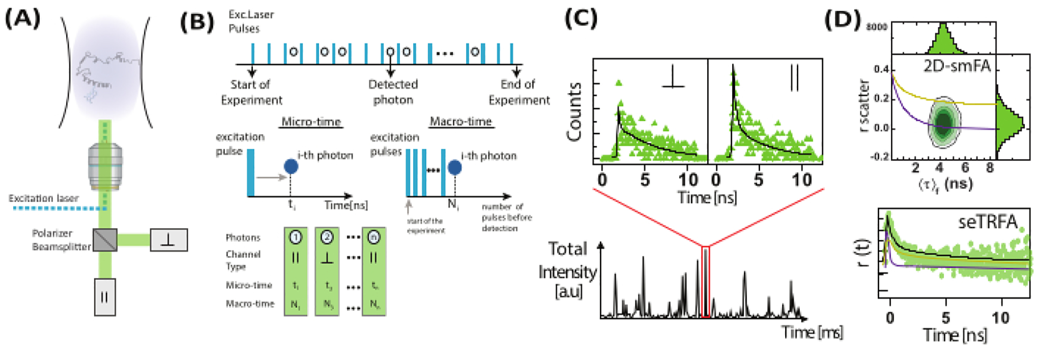
(A) Freely diffusing molecules are analyzed using a confocal single-molecule microscope equipped with a single linearly polarized excitation laser (blue in our case). Fluorescence emission (green in our case) is detected by two detectors after a beam polarizer splits the signal into two polarizations (parallel, ∥, and perpendicular, ⟘, to the excitation source). (B) Each detected photon is characterized by three parameters: micro time, macro time, and channel type. The data is stored in a Time-Tagged Time-Resolved (TTTR) format⁷². (C) Bursts of individual molecules are selected and processed to extract fluorescence parameters, including fluorescence anisotropy for each observed molecule. (D) Data is represented in multiple ways, including two-dimensional plots of fluorescence anisotropy versus fluorescence lifetime and time-resolved anisotropy decays. These representations allow for both visual and quantitative determination of fluorescence lifetimes, rotational correlation times, and system heterogeneity.

To consider the depolarizing effects of the high numerical aperture objective in a confocal microscope⁶², the proper form of the time-resolved anisotropy^35,63 is given by

$$r_{xy}\left(t\right)=\frac{G_{UV}{F}_{xy,\Vert }\left(t\right)-F_{xy,\perp }\left(t\right)}{\left(1-3l_2\right)G_{UV}{F}_{xy,\Vert }\left(t\right)+\left(2-3l_1\right)F_{xy,\perp }\left(t\right)}$$ (1)

where $F_{xy,\Vert }\left(t\right)$ and $F_{xy,\perp }\left(t\right)$ are the time-resolved fluorescence intensity in the y-th detection channel after excitation at the wavelength $x$, for the parallel and perpendicular polarization $l_1$ and $l_2$ and are factors that describe the mixing between the parallel and perpendicular signals due to the high numerical aperture (NA) objective used in these measurements^35,62,64. Differences in detection efficiencies of the parallel, ${\eta }_V^{{\lambda }_{emV,\Vert }}$, and perpendicular detection channel, ${\eta }_V^{{\lambda }_{emV,\perp }}$, for the dye are corrected with the ratio of the detection efficiencies, $G_{UV}=\frac{{\eta }_V^{{\lambda }_{emV,\perp }}}{{\eta }_V^{{\lambda }_{emV,\Vert }}}$. The $G_{UV}$ is also referred to as the G-factor.

The time-resolved fluorescence anisotropy can be modeled using a multiexponential decay to account for the fluorophore being attached to a larger biomolecule as

$$r_{xy}\left(t\right)=\left[\left(r_0-r_{\infty }\right)e^{\left(-\frac{t}{{\rho }_1}\right)}+r_{\infty }\right]e^{\left(-\frac{t}{{\rho }_2}\right)},$$ (2)

where $r_0$ is fluorophore dependent fundamental anisotropy (typically $r_0=0.38),r_{\infty }$ is the residual anisotropy, and ${\rho }_1$ and ${\rho }_2$ are fast (local motions of the fluorophore) and slow (global motion of the macromolecule) rotational correlation times, respectively.

In single-molecule anisotropy measurements (Figure 2), photon arrival times are recorded to identify individual emitters using burst-integrated fluorescence lifetime (BIFL) analysis^33,35. The inter-photon arrival times (Δt) are smoothed using a running average and then plotted to aid visualization. The histogram of these times is fitted with a half Gaussian to determine the mean and standard deviation of photons originating from the background. An arbitrary threshold, set at multiples of the standard deviation, is used to filter out individual events while identifying the first and last photons in each burst. Photons within each burst are then integrated for further analysis, which includes calculating time-resolved and intensity-based steady-state fluorescence anisotropy using equations 1 and 2 or via a maximum likelihood estimator³⁵. Due to the limited number of photons in single-molecule events, the maximum likelihood estimator considers only a single exponential component and will not be further discussed.

In a two-dimensional histogram of single molecule events, the mean fluorescence lifetime $\left(\tau \right)$ and anisotropy $\left(r_{xy}\right)$ can be related by Perrin’s equation^29,61 for obtaining $\left(\rho \right)$ as an average rotational time.

$$r_{xy}=\frac{r_0}{1+\frac{\langle \tau \rangle }{\langle \rho \rangle }}$$ (3)

Specific $\rho$ values can be obtained with higher certainty by “sub-ensemble” (se) analysis where the photons of different bursts are integrated into a combined time-resolved fluorescence anisotropy decay that can be analyzed by optimizing parameters of equation 2 to the experimental decay (seTRFA). Time-resolved anisotropy can resolve heterogeneity and dynamics associated with rotational motions (local and global) of the biomolecules within the emission of fluorescence that occurs within the ns timeframe.

To detect dynamics within single molecule events (on the submillisecond scale), we introduced time-resolved anisotropy Burst Variance Analysis (traBVA)⁵⁷. In traBVA, for a photon burst containing $M_i$ consecutive photon segments, the excess anisotropy variance $\left(s^2\right)$ for bursts is

$$s^2=\frac{1}{\left({\sum }_{i=1}^N{M}_i\right)-1}{\sum }_{i=1}^N{\sum }_{j=1}^{M_i}{\left(r_{xy,ij}-\langle r_{xy}\rangle \right)}^2.$$ (4)

For a single anisotropic state, the variance ${\sigma }^2$ arises solely from shot noise⁶⁵ (sn: $\surd N$, where $N$ is the number of photons)

$${\sigma }^2=\frac{\langle r_{xy}\rangle \left(1-\langle r_{xy}\rangle \right)}{m}$$ (5)

where m is the number of photons in a burst. Hence, to identify additional variance in the anisotropy, we can define the excess anisotropy variance $\left(S^2\right)$ due to conformational heterogeneity as the difference between equations 4 and 5.

$$S^2=s^2-{\sigma }^2$$ (6)

To capture dynamics that occur within the observation of individual molecules and consider the variance approximation, dynamic anisotropy Photon Distribution Analysis (daPDA)^55,56 can be used. In daPDA, the fluorescence intensity is modeled by following a conditional probability $\left(P\left(F_{xy,\Vert ,}{F}_{xy,\perp }\right)\right)$ expressed as a binomial distribution.

$$P\left(F_{xy,\Vert },F_{xy,\Vert }\mid F\right)=\frac{F_{xy}!}{F_{xy,\Vert }!F_{xy,\perp }!}{p}_{\Vert }^{F_{xy,\Vert }}{p}_{\perp }^{F_{xy,\perp }}$$ (7)

Together, with an estimate of the background count rate that follows a Poisson distribution

$$P\left(B\right)=\frac{{\langle B\rangle }^B\text{exp}\left(-\langle B\rangle \right)}{B!}$$ (8)

where $⟨B⟩$ is the average number of background photons per set time window. The parallel and perpendicular background counts, $⟨B_{\Vert }⟩$ and $⟨B_{\perp }⟩$, can be measured using buffer samples as a reference. The experimentally determined fluorescence anisotropy is optimized by minimizing a figure of merit ${\chi }^2$ with a fluorescence intensity distribution per polarization channel that can include kinetic changes.

The analysis routines and data representations provided offer a comprehensive approach to interpreting the collected data. Although this protocol primarily focuses on confocal measurements, which are limited in capturing anisotropy changes from nanoseconds to milliseconds, it is possible to adopt a Total Internal Reflection microscope to monitor fluorescence anisotropy over longer timescales, enabling time series analysis⁶⁶. For single-molecule confocal measurements, we highlight the use of multidimensional histograms that create a unique fingerprint of the observed ensemble. Time-resolved fluorescence decays, reconstructed from selected populations, can track the evolution of fluorescence anisotropy at the nanosecond scale (Figure 3). Photon distribution analysis^55,56 and burst variance analysis (BVA)^57,58 can also capture dynamics at intermediate timescales between time-resolved decays and multidimensional histograms. While this protocol does not cover the use of polarization fluorescence correlation spectroscopy (FCS), with or without pulsed excitation^67,68, which can bridge the nanosecond to millisecond timescales, the same data can be used to compute FCS⁶⁹, though this falls outside the scope of the presented protocol. If such experiments are undertaken, longer sample measurement time is recommended.

Figure 3: Representative data for FoxP1 domain-swapped dimer.

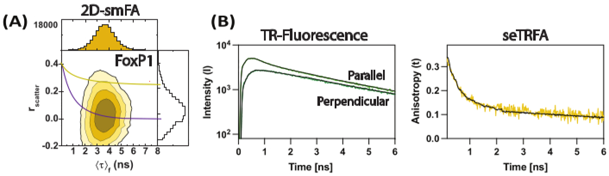
(A) Correlation of the fluorescence anisotropy $\left(r_{\mathit{\text{scatter}}}\right)$ against the mean fluorescence lifetime per molecule as a contour plot. Overlay of a single Perrin equation for two rotational components as a representative of the ensemble average of the molecule, considering ${\rho }_1$ and ${\rho }_2$ of 0.2 ns and 8.5 ns, respectively. (B) Sub-ensemble time-resolved fluorescence decays are used to compute the time-resolved fluorescence anisotropy of the sample. Fit with equation 2 resolved the local and global components of fluorescence anisotropy.

This approach has been applied to a complex system like the human FoxP proteins, providing valuable insights into the motions involved in their mechanism of action. FoxP proteins are transcription factors involved in several physiological aspects such as brain and lung development; importantly, different mutations have been recognized as impairing the function of these proteins^70,71. Using the DNA-binding domain of FoxP1 as a model, we generated different single-cysteine mutants to introduce a BODIPY-FL dye as a tracker for motions (Figure 4A). In fact, we evaluated the effect of dimerization and the DNA binding as major structural regulators of this protein. Using the smFA approach, we generated 2D-smFA plots and made traBVA and daPDA for each mutant in monomeric and dimeric conditions. We show an example of one of the single mutants studied (Figure 4). The anisotropy behavior is similar in all mutants in terms of determining high and low rotational correlation times and, therefore, presumable, disordered, and folded ensembles. Still, it is also highly heterogeneous in all mutants in terms of the fraction and kinetics of each ensemble, evidencing different order-to-disorder transition changes influenced by the dimerization and the DNA-binding, and shows the description at high resolution of the structural dynamics along the chain (Figure 5).

Figure 4: Sub-millisecond FoxP1 dynamics monitored using single-molecule fluorescence anisotropy (smFA).

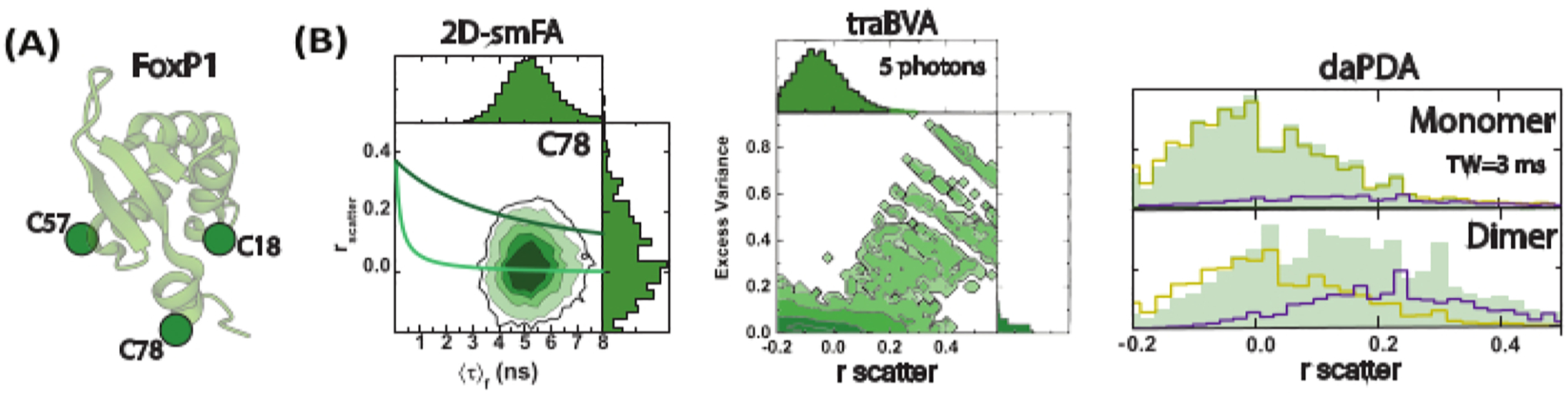
(A) A cartoon representation of the monomeric FoxP1 structure. (B) A two-dimensional histogram illustrates dynamic heterogeneity, revealing two distinct rotational correlation times identified through time-resolved fluorescence anisotropy. Time-resolved anisotropy Burst Variance Analysis (traBVA) uncovers a small subset of events with excess variance (Eq. 6) that exhibit large anisotropy. Quantitative dynamic anisotropy analysis using Photon Distribution Analysis (PDA) further extracts the exchange rates for this process.

Figure 5: Screening the local and global motions of FoxP1 during dimerization.

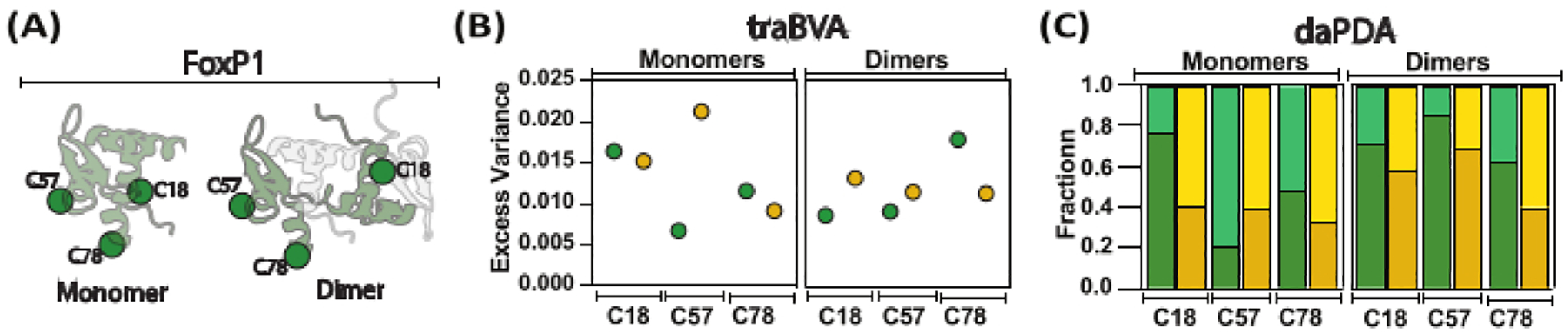
(A) A cartoon representation compares the monomeric FoxP1 with its dimeric form. (B) Mean excess variance per location under monomeric and dimeric conditions is shown, with larger excess variance indicating more significant changes in anisotropy. (C) Dynamic anisotropy analysis using Photon Distribution Analysis (PDA) helps determine population fractions (high anisotropy in dark colors and low anisotropy in light color) in the absence (green) and presence (yellow) of DNA. In this approach, rates (not shown) were estimated for transitions between local and global behaviors, revealing that FoxP1 undergoes partial unfolding.

Discussion

For single-molecule fluorescence anisotropy experiments, it is crucial to consider the chosen fluorophore’s photophysical properties carefully. These properties include the emission wavelength, which must align with the detection system, and the excitation wavelength, which should be compatible with the available pulsed lasers. To optimize the dynamic range, the fluorophore should have a long fluorescence lifetime relative to the molecule’s rotational diffusion time. This is critical for tracking rotational dynamics and the linkage/orientation of the fluorophore’s dipole relative to the biomolecule of interest. Additionally, brightness, photostability, and quantum yield are essential for producing strong signals with a stable signal-to-noise ratio. For these reasons, BODIPY-FL has been chosen as the fluorophore in several studies^39,40,42.

Screening the backbone dynamics of biomolecules often requires protein labeling, typically achieved through site-specific labeling. This is usually done by introducing a residue for targeted chemical modification. The most common approach is introducing cysteines at positions of interest, where their thiol side chains can be selectively modified with reagents such as maleimides or iodoacetamides. Less commonly, benzylic halides and bromomethyl ketones are used to form thioether bonds. Other amino acid side chains can also be targeted, but their abundance in proteins is less commonly used. However, alternative approaches, like unnatural amino acids, can also be used⁷³. Proper site selection for labeling is crucial to minimize interference with the biomolecule under study, and appropriate controls must be in place. For example, if the labeled molecule is used in binding assays, complementary label-free methods should verify that the fluorophores do not impact binding affinity.

After identifying the appropriate sample and implementing the optimal labeling strategy, the next step is to ensure the confocal microscope is properly aligned and calibrated for single-molecule experiments. The protocol describes how to determine the required factor for further analysis. Once the instrument is calibrated, the next step is to measure the sample and process the data to extract as much information as possible from the detected photons. The key parameters, such as micro-time, macro-time, and channel type, as shown in Figure 2, can be used for further analysis and visualization using typical TCSPC electronics.

Recent advances in single-molecule fluorescence spectroscopy can be extensively used to study structural information from the heterogeneous ensembles of biomolecules. However, relatively few studies leverage the insights provided by fluorescence anisotropy, and a complete protein model is required to derive the structural dynamics of biomolecules. Therefore, unraveling the dynamics of interdomain and protein-protein interactions of several transcription factors is challenging.

In conclusion, single-molecule fluorescence anisotropy experiments offer complementary information about the local and global motions of the biomolecular backbone, which are critical for understanding its function.

Materials

Name	Company	Catalog Number	Comments
Alexa Fluor 488	ThermoFisher Scienctific	A20100	https://www.thermofisher.com/order/catalog/product/A20100?SID=srch-srp-A20100
Amicon Ultra Centrifugal Filter, 10 kDa MWCO	Millipore Sigma	UFC901008	https://www.sigmaaldrich.com/US/en/product/mm/ufc9010
Ampicillin sodium salt	Millipore Sigma	A0166-5G	https://www.sigmaaldrich.com/US/en/product/sigma/a0166
BODIP FL Maleimide (BODIPY FL N-(2-Aminoethyl))Maleimide)	ThermoFisher Scienctific	B10250	https://www.thermofisher.com/order/catalog/product/B10250?SID=srch-srp-B10250
Disposable PD 10 Desalting Columns	Millipore Sigma	GE17-0851-01	https://www.sigmaaldrich.com/US/en/product/sigma/ge17085101
Dithiothreitol	Millipore Sigma	10197777001	https://www.sigmaaldrich.com/US/en/product/roche/dttro
DMSO, Anhydrous	ThermoFisher Scienctific	D12345	https://www.thermofisher.com/order/catalog/product/D12345?SID=srch-srp-D12345
DNAse	Millipore Sigma	10104159001	https://www.sigmaaldrich.com/US/en/product/roche/10104159001
E. coli C41 bacterial cells	Invitrogen
Foresigh Nuvi Ni-Charged IMAC, 5 mL column	Bio-Rad	12004037	https://www.bio-rad.com/en-us/sku/12004037-foresight-nuvia-ni-charged-imac-5-ml-column?ID=12004037
HEPES	Millipore Sigma	7365-45-9	https://www.sigmaaldrich.com/US/en/product/sigma/h3375
Imidazole	Millipore Sigma	288-32-4	https://www.sigmaaldrich.com/US/en/product/sigma/i5513
IPTG	Millipore Sigma	I6758-1G	https://www.sigmaaldrich.com/US/en/product/sial/i6758
MCE Membrane Filter, 0.22 μm Pore Size	Millipore Sigma	GSWP02500	https://www.sigmaaldrich.com/US/en/product/mm/gswp02500
NaCl	Millipore Sigma	7647-14-5	https://www.sigmaaldrich.com/US/en/product/sigma/s3014
Nunc Lab-Tek II Chamber Slide System	ThermoFisher Scienctific	154534	https://www.thermofisher.com/order/catalog/product/154534
OverExpress C41(DE3) Chemically Competent Cells	Millipore Sigma	CMC0017-20X40UL	https://www.sigmaaldrich.com/US/en/product/sigma/cmc0017
PMSF	Millipore Sigma	329-98-6	https://www.sigmaaldrich.com/US/en/product/sigma/78830
Rhodamine 110	ThermoFisher Scienctific	419075000	https://www.thermofisher.com/order/catalog/product/419075000?SID=srch-hj-419075000
Sodium phosphate dibasic	Millipore Sigma	7558-79-4	https://www.sigmaaldrich.com/US/en/product/sigma/s3264
Sodium phosphate monobasic dihydrate	Millipore Sigma	13472-35-0	https://www.sigmaaldrich.com/US/en/product/sigma/71505
TCEP, Hydrochloride, Reagent Grade	Millipore Sigma	580567-5GM	https://www.sigmaaldrich.com/US/en/product/mm/580567
Tween 20	Millipore Sigma	11332465001	https://www.sigmaaldrich.com/US/en/product/roche/11332465001

References

- 1.Cooper A Thermodynamic fluctuations in protein molecules. Proc Natl Acad Sci U S A. 73 (8), 2740–2741 (1976). [DOI] [PMC free article] [PubMed] [Google Scholar]
- 2.Volozhin SI Inguinal hernia in cryptorchism. Khirurgiia (Mosk). 450 (7), 69–71 (1975). [PubMed] [Google Scholar]
- 3.Henzler-Wildman KA et al. Intrinsic motions along an enzymatic reaction trajectory. Nature. 450 (7171), 838–844 (2007). [DOI] [PubMed] [Google Scholar]
- 4.Karplus M Mccammon JA The internal dynamics of globular-proteins. CRC Crit Rev Biochem. 9 (4), 293–349 (1981). [DOI] [PubMed] [Google Scholar]
- 5.Ishima R Torchia DA Protein dynamics from nmr. Nat Struct Biol. 7 (9), 740–743 (2000). [DOI] [PubMed] [Google Scholar]
- 6.Fernandez FJ, Querol-Garcia J, Navas-Yuste S, Martino F, Vega MC X-ray crystallography for macromolecular complexes. Adv Exp Med Biol. 3234, 125–140 (2024). [DOI] [PubMed] [Google Scholar]
- 7.Bai XC, Mcmullan G, Scheres SH How cryo-EM is revolutionizing structural biology. Trends Biochem Sci. 40 (1), 49–57 (2015). [DOI] [PubMed] [Google Scholar]
- 8.Wright PE Dyson HJ Intrinsically unstructured proteins: Re-assessing the protein structure-function paradigm. J Mol Biol. 293 (2), 321–331 (1999). [DOI] [PubMed] [Google Scholar]
- 9.Tompa P Intrinsically unstructured proteins. Trends Biochem Sci. 27 (10), 527–533 (2002). [DOI] [PubMed] [Google Scholar]
- 10.Dyson HJ Wright PE Intrinsically unstructured-proteins and their functions. Nat Rev Mol Cell Biol. 6 (3), 197–208 (2005). [DOI] [PubMed] [Google Scholar]
- 11.Csermely P, Palotai R, Nussinov R Induced fit, conformational selection and independent dynamic segments: An extended view of binding events. Trends Biochem Sci. 35 (10), 539–546 (2010). [DOI] [PMC free article] [PubMed] [Google Scholar]
- 12.Camacho-Zarco AR et al. NMR provides unique insight into the functional dynamics and interactions of intrinsically disordered proteins. Chem Rev. 122 (10), 9331–9356 (2022). [DOI] [PMC free article] [PubMed] [Google Scholar]
- 13.Drenth J Principles of Protein X-Ray Crystallography. Springer, Verlag, New York, NY: (2007). [Google Scholar]
- 14.Loeb H Systematic diagnosis of chronic diarrhea in infants and small children. Kinderarztl Prax. 44 (1), 36–41 (1976). [PubMed] [Google Scholar]
- 15.Ellaway JIJ et al. Identifying protein conformational states in the protein data bank: Toward unlocking the potential of integrative dynamics studies. Struct Dyn. 11 (3), 034701 (2024). [DOI] [PMC free article] [PubMed] [Google Scholar]
- 16.Berjanskii MV Wishart DS A simple method to predict protein flexibility using secondary chemical shifts. J Am Chem Soc. 127 (43), 14970–14971 (2005). [DOI] [PubMed] [Google Scholar]
- 17.Puthenveetil R Vinogradova O Solution NMR: A powerful tool for structural and functional studies of membrane proteins in reconstituted environments. J Biol Chem. 294 (44), 15914–15931 (2019). [DOI] [PMC free article] [PubMed] [Google Scholar]
- 18.Wozniak AK, Schroder GF, Grubmuller H, Seidel CA, Oesterhelt F Single-molecule fret measures bends and kinks in DNA. Proc Natl Acad Sci U S A. 105 (47), 18337–18342 (2008). [DOI] [PMC free article] [PubMed] [Google Scholar]
- 19.Weidtkamp-Peters S et al. Multiparameter fluorescence image spectroscopy to study molecular interactions. Photochem Photobiol Sci. 8 (4), 470–480 (2009). [DOI] [PubMed] [Google Scholar]
- 20.Sisamakis E, Valeri A, Kalinin S, Rothwell PJ, Seidel CAM Accurate single-molecule FRET studies using multiparameter fluorescence detection. Methods Enzymol. 475, 455–514 (2010). [DOI] [PubMed] [Google Scholar]
- 21.Kalinin S et al. A toolkit and benchmark study for fret-restrained high-precision structural modeling. Nat Methods. 9 (12), 1218–1225 (2012). [DOI] [PubMed] [Google Scholar]
- 22.Peulen TO, Opanasyuk O, Seidel C.a. M. Combining graphical and analytical methods with molecular simulations to analyze time-resolved fret measurements of labeled macromolecules accurately. J Phys Chem B. 121 (35), 8211–8241 (2017). [DOI] [PMC free article] [PubMed] [Google Scholar]
- 23.Hamilton GL Sanabria H Multiparameter Fluorescence Spectroscopy of Single Molecules. In Spectroscopy and Dynamics of Single Molecules. Elsevier, Cambridge, MA: (2019). [Google Scholar]
- 24.Kolimi N et al. Out-of-equilibrium biophysical chemistry: The case for multidimensional, integrated single-molecule approaches. J Phys Chem B. 125 (37), 10404–10418 (2021). [DOI] [PMC free article] [PubMed] [Google Scholar]
- 25.Felekyan S, Sanabria H, Kalinin S, Kuhnemuth R, Seidel CA Analyzing forster resonance energy transfer with fluctuation algorithms. Methods Enzymol. 519, 39–85 (2013). [DOI] [PubMed] [Google Scholar]
- 26.Medina E, D RL, Sanabria H Unraveling protein’s structural dynamics: From configurational dynamics to ensemble switching guides functional mesoscale assemblies. Curr Opin Struct Biol. 66, 129–138 (2021). [DOI] [PMC free article] [PubMed] [Google Scholar]
- 27.Aznauryan M et al. Comprehensive structural and dynamical view of an unfolded protein from the combination of single-molecule FRET, NMR, and SAXS. Proc Natl Acad Sci U S A. 113 (37), E5389–E5398 (2016). [DOI] [PMC free article] [PubMed] [Google Scholar]
- 28.Gomes GW et al. Conformational ensembles of an intrinsically disordered protein consistent with NMR, SAXS, and single-molecule fret. J Am Chem Soc. 142 (37), 15697–15710 (2020). [DOI] [PMC free article] [PubMed] [Google Scholar]
- 29.Perrin F Polarisation de la lumière de fluorescence. Vie moyenne des molécules dans l’etat excité. J phys radium. 7 (12), 390–401 (1926). [Google Scholar]
- 30.Weber G Polarization of the fluorescence of macromolecules. I. Theory and experimental method. Biochem J. 51 (2), 145–155 (1952). [DOI] [PMC free article] [PubMed] [Google Scholar]
- 31.Weber G Polarization of the fluorescence of macromolecules. II. Fluorescent conjugates of ovalbumin and bovine serum albumin. Biochem J. 51 (2), 155–167 (1952). [DOI] [PMC free article] [PubMed] [Google Scholar]
- 32.Jameson DM Ross JA Fluorescence polarization/anisotropy in diagnostics and imaging. Chem Rev. 110 (5), 2685–2708 (2010). [DOI] [PMC free article] [PubMed] [Google Scholar]
- 33.Eggeling C, Fries JR, Brand L, Gunther R, Seidel CA Monitoring conformational dynamics of a single molecule by selective fluorescence spectroscopy. Proc Natl Acad Sci U S A. 95 (4), 1556–1561 (1998). [DOI] [PMC free article] [PubMed] [Google Scholar]
- 34.Fries JR, Brand L, Eggeling C, Köllner M, Seidel C. a. M. Quantitative identification of different single molecules by selective time-resolved confocal fluorescence spectroscopy. Journal of Physical Chemistry A. 102 (33), 6601–6613 (1998). [Google Scholar]
- 35.Schaffer J et al. Identification of single molecules in aqueous solution by time-resolved fluorescence anisotropy. Journal of Physical Chemistry A. 103 (3), 331–336 (1999). [Google Scholar]
- 36.Widengren J et al. Single-molecule detection and identification of multiple species by multiparameter fluorescence detection. Anal Chem. 78 (6), 2039–2050 (2006). [DOI] [PubMed] [Google Scholar]
- 37.Gradinaru CC, Marushchak DO, Samim M, Krull UJ Fluorescence anisotropy: From single molecules to live cells. Analyst. 135 (3), 452–459 (2010). [DOI] [PubMed] [Google Scholar]
- 38.Mazal H Haran G Single-molecule fret methods to study the dynamics of proteins at work. Curr Opin Biomed Eng. 12, 8–17 (2019). [DOI] [PMC free article] [PubMed] [Google Scholar]
- 39.Tsytlonok M et al. Specific conformational dynamics and expansion underpin a multi-step mechanism for specific binding of p27 with cdk2/cyclin a. J Mol Biol. 432 (9), 2998–3017 (2020). [DOI] [PMC free article] [PubMed] [Google Scholar]
- 40.Tsytlonok M et al. Dynamic anticipation by cdk2/cyclin a-bound p27 mediates signal integration in cell cycle regulation. Nat Commun. 10 (1), 1676 (2019). [DOI] [PMC free article] [PubMed] [Google Scholar]
- 41.Cruz P et al. Domain tethering impacts dimerization and DNA-mediated allostery in the human transcription factor foxp1. J Chem Phys. 158 (19), (2023). [DOI] [PMC free article] [PubMed] [Google Scholar]
- 42.Kolimi N et al. DNA controls the dimerization of the human foxp1 forkhead domain. Cell Rep Phys Sci. 5 (3), 101854 (2024). [DOI] [PMC free article] [PubMed] [Google Scholar]
- 43.Yanez Orozco IS et al. Identifying weak interdomain interactions that stabilize the supertertiary structure of the n-terminal tandem PDZ domains of PSD-95. Nat Commun. 9 (1), 3724 (2018). [DOI] [PMC free article] [PubMed] [Google Scholar]
- 44.Elson EL Magde D Fluorescence correlation spectroscopy. I. Conceptual basis and theory. Biopolymers. 13 (1), 1–27 (1974). [DOI] [PubMed] [Google Scholar]
- 45.Rigler R Elson ES Fluorescence Correlation Spectroscopy: Theory and Applications. Springer, Berlin, Heidelberg: (2012). [Google Scholar]
- 46.Aragon SR Pecora R Fluorescence correlation spectroscopy as a probe of molecular-dynamics. J Chem Phys. 64 (4), 1791–1803 (1976). [Google Scholar]
- 47.Mockel C et al. Integrated NMR, fluorescence, and molecular dynamics benchmark study of protein mechanics and hydrodynamics. J Phys Chem B. 123 (7), 1453–1480 (2019). [DOI] [PubMed] [Google Scholar]
- 48.Shu W, Yang H, Zhang L, Lu MM, Morrisey EE Characterization of a new subfamily of winged-helix/forkhead (Fox) genes that are expressed in the lung and act as transcriptional repressors. J Biol Chem. 276 (29), 27488–27497 (2001). [DOI] [PubMed] [Google Scholar]
- 49.Co M, Anderson AG, Konopka G Foxp transcription factors in vertebrate brain development, function, and disorders. Wiley Interdiscip Rev Dev Biol. 9 (5), e375 (2020). [DOI] [PMC free article] [PubMed] [Google Scholar]
- 50.Takahashi H, Takahashi K, Liu F-C FOXP Genes, Neural Development, Speech and Language Disorders. In Forkhead Transcription Factors: Vital Elements in Biology and Medicine. Springer, New York, NY: (2009). [DOI] [PubMed] [Google Scholar]
- 51.Wang B, Lin D, Li C, Tucker P Multiple domains define the expression and regulatory properties of foxp1 forkhead transcriptional repressors. J Biol Chem. 278 (27), 24259–24268 (2003). [DOI] [PubMed] [Google Scholar]
- 52.Leake MC Quinn SD A guide to small fluorescent probes for single-molecule biophysics. Chem Phys Rev. 4 (1), 011302 (2023). [Google Scholar]
- 53.Zhang H, Wu Q, Berezin MY Fluorescence anisotropy (polarization): From drug screening to precision medicine. Expert Opin Drug Discov. 10 (11), 1145–1161 (2015). [DOI] [PMC free article] [PubMed] [Google Scholar]
- 54.Ma J et al. High precision fret at single-molecule level for biomolecule structure determination. J Vis Exp. 123, e55623 (2017). [DOI] [PMC free article] [PubMed] [Google Scholar]
- 55.Antonik M, Felekyan S, Gaiduk A, Seidel CA Separating structural heterogeneities from stochastic variations in fluorescence resonance energy transfer distributions via photon distribution analysis. J Phys Chem B. 110 (13), 6970–6978 (2006). [DOI] [PubMed] [Google Scholar]
- 56.Mcgeer PL Mcgeer EG Enzymes associated with the metabolism of catecholamines, acetylcholine and gaba in human controls and patients with parkinson’s disease and huntington’s chorea. J Neurochem. 26 (1), 65–76 (1976). [PubMed] [Google Scholar]
- 57.Terterov I, Nettels D, Makarov DE, Hofmann H Time-resolved burst variance analysis. Biophys Rep (N Y). 3 (3), 100116 (2023). [DOI] [PMC free article] [PubMed] [Google Scholar]
- 58.Torella JP, Holden SJ, Santoso Y, Hohlbein J, Kapanidis AN Identifying molecular dynamics in single-molecule fret experiments with burst variance analysis. Biophys J. 100 (6), 1568–1577 (2011). [DOI] [PMC free article] [PubMed] [Google Scholar]
- 59.Haugland RP The Handbook: A Guide to Fluorescent Probes and Labeling Technologies. Molecular Probes; (2005). [Google Scholar]
- 60.Medina E et al. Intrinsically disordered regions of the DNA-binding domain of human foxp1 facilitate domain swapping. J Mol Biol. 432 (19), 5411–5429 (2020). [DOI] [PMC free article] [PubMed] [Google Scholar]
- 61.Lakowicz JR Principles of Fluorescence Spectroscopy. Springer; New York, NY: (2007). [Google Scholar]
- 62.Koshioka M, Sasaki K, Masuhara H Time-dependent fluorescence depolarization analysis in three-dimensional microspectroscopy. Appl Spectrosc. 49 (2), 224–228 (1995). [Google Scholar]
- 63.Kudryavtsev V et al. Combining mfd and pie for accurate single-pair forster resonance energy transfer measurements. Chemphyschem. 13 (4), 1060–1078 (2012). [DOI] [PubMed] [Google Scholar]
- 64.Van Zanten TS, Greeshma PS, Mayor S Quantitative fluorescence emission anisotropy microscopy for implementing homo-fluorescence resonance energy transfer measurements in living cells. Mol Biol Cell. 34 (6), tp1 (2023). [DOI] [PMC free article] [PubMed] [Google Scholar]
- 65.Laine RF, Jacquemet G, Krull A Imaging in focus: An introduction to denoising bioimages in the era of deep learning. Int J Biochem Cell Biol. 140, 106077 (2021). [DOI] [PMC free article] [PubMed] [Google Scholar]
- 66.Strohl F, Wong HHW, Holt CE, Kaminski CF Total internal reflection fluorescence anisotropy imaging microscopy: Setup, calibration, and data processing for protein polymerization measurements in living cells. Methods Appl Fluoresc. 6 (1), 014004 (2017). [DOI] [PMC free article] [PubMed] [Google Scholar]
- 67.Loman A, Gregor I, Stutz C, Mund M, Enderlein J Measuring rotational diffusion of macromolecules by fluorescence correlation spectroscopy. Photochem Photobiol Sci. 9 (5), 627–636 (2010). [DOI] [PubMed] [Google Scholar]
- 68.Böhmer M, Wahl M, Rahn H-J, Erdmann R, Enderlein J Time-resolved fluorescence correlation spectroscopy. Chem Phys Lett. 353 (5–6), 439–445 (2002). [Google Scholar]
- 69.Peulen T-O et al. Tttrlib: Modular software for integrating fluorescence spectroscopy, imaging, and molecular modeling. arXiv. 2402.17252 (2024). [DOI] [PMC free article] [PubMed] [Google Scholar]
- 70.Le Fevre AK et al. Foxp1 mutations cause intellectual disability and a recognizable phenotype. Am J Med Genet A. 161A (12), 3166–3175 (2013). [DOI] [PubMed] [Google Scholar]
- 71.Hamdan FF et al. De novo mutations in foxp1 in cases with intellectual disability, autism, and language impairment. Am J Hum Genet. 87 (5), 671–678 (2010). [DOI] [PMC free article] [PubMed] [Google Scholar]
- 72.Wahl M Orthaus-Müller S Time tagged time-resolved fluorescence data collection in life sciences. At <https://www.picoquant.com/images/uploads/page/files/14528/technote_tttr.pdf> (2014).
- 73.Lemke EA Site-specific labeling of proteins for single-molecule fret measurements using genetically encoded ketone functionalities. Methods Mol Biol. 751, 3–15 (2011). [DOI] [PubMed] [Google Scholar]