Asymptotically scale-invariant occupancy of phase space makes the entropy S_q extensive

Abstract

Phase space can be constructed for N equal and distinguishable subsystems that could be probabilistically either weakly correlated or strongly correlated. If they are locally correlated, we expect the Boltzmann-Gibbs entropy S_BG ≡ -k Σ_i p_i ln p_i to be extensive, i.e., S_BG(N) ∝ N for N → ∞. In particular, if they are independent, S_BG is strictly additive, i.e., S_BG(N) = NS_BG(1), ∀N. However, if the subsystems are globally correlated, we expect, for a vast class of systems, the entropy S_q ≡ k[1 - Σ_i p^q_i]/(q - 1) (with S₁ = S_BG) for some special value of q ≠ 1 to be the one which is extensive [i.e., S_q(N) ∝ N for N → ∞]. Another concept which is relevant is strict or asymptotic scale-freedom (or scale-invariance), defined as the situation for which all marginal probabilities of the N-system coincide or asymptotically approach (for N → ∞) the joint probabilities of the (N - 1)-system. If each subsystem is a binary one, scale-freedom is guaranteed by what we hereafter refer to as the Leibnitz rule, i.e., the sum of two successive joint probabilities of the N-system coincides or asymptotically approaches the corresponding joint probability of the (N - 1)-system. The kinds of interplay of these various concepts are illustrated in several examples. One of them justifies the title of this paper. We conjecture that these mechanisms are deeply related to the very frequent emergence, in natural and artificial complex systems, of scale-free structures and to their connections with nonextensive statistical mechanics. Summarizing, we have shown that, for asymptotically scale-invariant systems, it is S_q with q ≠ 1, and not S_BG, the entropy which matches standard, clausius-like, prescriptions of classical thermodynamics.

The entropy S_q (1) is defined through§,¶

[1]

where k is a positive constant (k = 1 from now on) and BG stands for Boltzmann-Gibbs. This expression is the basis of nonextensive statistical mechanics (16-18) (see http://tsallis.cat.cbpf.br/biblio.htm for a regularly updated bibliography), a current generalization of BG statistical mechanics. For q ≠ 1, S_q is nonadditive (hence nonextensive) in the sense that for a system composed of (probabilistically) independent subsystems, the total entropy differs from the sum of the entropies of the subsystems. However, the system may have special probability correlations between the subsystems such that extensivity is valid, not for S_BG, but for S_q with a particular value of the index q ≠ 1. In this paper, we address the case where the subsystems are all equal and distinguishable. Their correlations may exhibit a kind of scale-invariance. We may regard some of the situations of correlated probabilities as related to the remark (see refs. 19-23 and references therein) that S_q for q ≠ 1 can be appropriate for nonlinear dynamical systems that have phase space unevenly occupied. We return to this point later.

We shall consider two types of models. The first one involves N binary variables (N = 1, 2, 3,...), and the second one involves N continuous variables (N = 1, 2, 3). In both cases, certain correlations that are scale-invariant in a suitable limit can create an intrinsically inhomogeneous occupation of phase space. Such systems are strongly reminiscent of the so called scale-free networks (24, 25), with their hierarchically structured hubs and spokes and their nearly forbidden regions.

Discrete Models

Some Basic Concepts. The most general probabilistic sets for N equal and distinguishable binary subsystems are given in Fig. 1 with

[2]

Fig. 1.

Most general sets of joint probabilities for N equal and distinguishable binary subsystems.

Let us from now on call Leibnitz rule the following recursive relation:

[3]

This relation guarantees what we refer to as scale-invariance (or scale-freedom) in this article. Indeed, it guarantees that, for any value of N, the associated joint probabilities {π_N,n} produce marginal probabilities which coincide with {π_N-1,n}. Assuming π₁₀ + π₁₁ = 1, and taking into account that the Nth row has one more element than the (N - 1)th row, a particular model is characterized by giving one element for each row. We shall adopt the convention of specifying the set {π_N,0 ∈ [0, 1], ∀N}. Everything follows from it. There are many sets {π_N,0} that satisfy Eq. 3. Let us illustrate with a few simple examples:

(i) π_N,0 = (2π₁₀)^N/N + 1 (0 ≤ π₁₀ ≤ 1/2; N = 1, 2, 3,...). We have that all 2^N states have nonzero probability if 0 < π₁₀ ≤ 1/2. The particular case π₁₀ = 1/2 recovers the original Leibnitz triangle itself (26) (see Fig. 2).

Fig. 2.

The left numbers within the parentheses correspond to Pascal triangle. The right numbers correspond to the Leibnitz harmonic triangle (d = N).

(ii) π_N,0 = (π₁₀)^Nα (α ≥ 0; N = 1, 2, 3...). The α = 1 instance corresponds to independent systems, i.e., π_N,n = (π₁₀)^N-n (1 - π₁₀)ⁿ. If 0 < π₁₀ < 1, then all 2^N states have nonzero probability. The α = 0 instance corresponds to π_N,0 = π₁₀, π_N,n = 0 (n = 1, 2,..., N - 1) and π_N,N = 1 - π₁₀. If 0 < π₁₀ < 1, then only two among the 2^N states have nonzero probability, ∀N, namely the states associated with π_N,0 and π_N,N.

We may relax the Leibnitz rule to some extent by considering those cases where the rule is satisfied only asymptotically, i.e.,

[4]

Such cases will be said to be not strictly but asymptotically scale-invariant (or asymptotically scale-free). This is, for a variety of reasons, the situation in which we are primarily interested. The main reason is that what vast classes of natural and artificial systems typically exhibit is not precisely power-laws, but behaviors which only asymptotically become power-laws (once we have corrected, of course, for any finite size effects). This is consistent with the fact that within nonextensive statistical mechanics S_q is optimized by q-exponential functions (see ref. 1 and references therein and refs. 27 and 28), which only asymptotically yield power-laws. It is consistent also with a new central limit theorem that has been recently conjectured (29) for specially correlated random variables.∥

Let us now introduce a further concept, namely q-describability. A model constituted by N equal and distinguishable subsystems will be called q-describable if a value of q exists such as S_q(N)is extensive, i.e., lim_N→∞ S_q(N)/N <∞. If that special value of q equals unity, this corresponds to the usual BG universality class. If that value of q differs from unity, we will have nontrivial universality classes. If the subsystems {A_i} are not necessarily equal, the system is q-describable if an entropic index q exists such that lim_N→∞ . It should be clear that we could equally well demand the extensivity of say S_2-q [or even of S_Q(q), where Q(q) is some monotonically decreasing function of q satisfying Q(1) = 1] instead of that of S_q. This would of course have the effect of having nontrivial solutions for q > 1 whenever we had solutions for q < 1 if the extensivity that was imposed was that of S_q.

Finally, let us point out that we might consider the subsystems of a probabilistic system to be either strongly (or globally) correlated or weakly (or “locally”) correlated. The trivial case of independence, i.e., when the subsystems are uncorrelated, is of course a particular case of weakly correlated. Let us make these notions more precise. A system is weakly correlated if for every generic (different from zero and from unity) joint probability a set of individual probabilities exists such that lim_N→∞ . Otherwise, the system is said to be strongly correlated. The particular case of independence corresponds to

If the subsystems are equal and binary, this definition becomes as follows: a system is weakly correlated if, for generic π_N,n, a probability p₀ exists such that lim_N→γ . Otherwise the system is said to be strongly correlated. The particular case of independence corresponds to p₀ = π₁₀. In the present sense, weakly correlated systems could also be thought and referred to as asymptotically uncorrelated. The interplay of scale-invariance, q-describability, and global correlation is schematized in Fig. 3.

Fig. 3.

Scheme representing the systems that are q-describable, globally correlated, asymptotically scale-free (ASF), and strictly scale-free (SSF). The q = 1 region corresponds to “locally” correlated systems. The Leibnitz rule is strictly satisfied for SSF, but only asymptotically satisfied for ASF. Below (above) the continuous red line we have the ASF (non ASF) systems. The SSF systems (below the dashed red line) constitute a subset of the ASF subset. The red spots correspond to the four families of discrete systems illustrated in the present paper: q ≠ 1 non ASF (upper spot; Eqs. 12 and 14); q ≠ 1 ASF but non SSF (middle spot; Eqs. 17 and 24); q ≠ 1 SSF (right bottom spot; Eq. 8); q = 1 SSF (left bottom spot; examples i and ii in the text).

We have verified that all systems illustrated in i and ii above belong to the q = 1 class (see examples in Fig. 4). We next address q ≠ 1 systems.

Fig. 4.

S_q(N) for the Leibnitz triangle [the explicit expression π_N,n = 1/(N + 1) (N - n)!n!/N! has been used to calculate S_q(N)] (a) α = 1 (i.e., independent subsystems) with π₁₀ = 1/2 [the explicit expression π_N,n = (π₁₀)^N-n (1 - π₁₀)ⁿ has been used to calculate S_q(N) (b) and α = 1/2 with π₁₀ = 1/2 [the recursive relation 3 has been used to calculated S_q(N)] (c). Only for q = 1 we have a finite value for lim_{N → ∞} S_q(N)/N; it vanishes (diverges) for q > 1 (q < 1).

A Discrete Model That Is Not Asymptotically Scale-Invariant. Let us consider the probabilistic structure indicated in Fig. 5, where, for given N, only the d + 1 first elements are different from zero, with d = 0, 1, 2,..., N.

Fig. 5.

Probabilistic models with d = 1 (Left) and d = 2 (Right).

As we see, for N ≥ d + 1 and n = d + 1, d + 2,..., N. The total number of states is given by W(N) = 2^N (∀d), but the number of states with nonzero probability is given by

[5]

where eff stands for effective. For example, W_eff(N, 0) = 1, W_eff(N, 1) = N + 1, W_eff(N, 2) = ½N(N + 1) + 1, W_eff(N, 3) = ⅙N(N² + 5) + 1, and so on. For fixed d and N → ∞ we have that

[6]

Let us now make a simple choice for the nonzero probabilities, namely equal probabilities. In other words,

[7]

See Fig. 6 for an illustration of this model.

Fig. 6.

Uniform distribution model with d = 1 (Left) and d = 2 (Right).

The entropy for this model is given by

[8]

where we have used now Eq. 6. Consequently, S_q is extensive [i.e., S_q(N) ∝ N for N → ∞] if and only if

[9]

Hence, if d = 1, 2, 3..., the entropic index monotonically approaches the BG limit from below. We can immediately verify in Fig. 6 (and using Eq. 7) that this model violates the Leibnitz rule for all N, including asymptotically when N → ∞. Consequently, it is neither strictly nor asymptotically scale-free. However, it is q-describable (see Fig. 3).

An Asymptotically Scale-Invariant Discrete Model. Starting with the Leibnitz harmonic triangle, we shall construct a heterogeneous distribution . The Leibnitz triangle is given in Fig. 2 and satisfies

[10]

[11]

We now define

[12]

where the excess probability and the distribution ratio (with 0 < ε < 1) are defined through

[13]

[14]

(see Fig. 7). We have verified for d = 1, 2, 3, 4 and N → ∞ a result that we expect to be correct for all d < N/2, namely that 0 < π_N,n+1 << π_N,n ∼ π_N-1,n << 1, hence

[15]

[16]

Fig. 7.

Leibnitz-triangle-based ε = 0.5 probability sets: d = 1 (Left), and d = 2 (Right).

In other words, the Leibnitz rule is asymptotically satisfied for the entire probability set {π_N,n}, i.e., this system has asymptotic scale invariance. Its entropy is given by

[17]

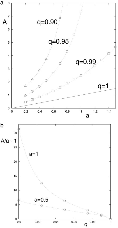
and we verify that a value of q exists such that lim_N→∞ S_q(N,d)/N is finite. Our numerical results suggest that, for 0 < ε < 1 (see Fig. 8),

[18]

Fig. 8.

Illustrations of the extensivity of S_q for the q ≠ 1 ASF model (with ε = 0.5): (a) d = 1; (b) d = 2; and (c) d = 3. Notice that the minimal value of N equals d - 1. lim_{N → ∞} S_q(N)/N vanishes (diverges) if q > 1 - 1/d (q < 1 - 1/d), whereas it is finite for q = 1 - 1/d.

For a description of a strictly scale-invariant discrete model and a continuous model, see Supporting Text and Figs. 9-17, which are published as supporting information on the PNAS web site.

Final Remarks

Let us now critically re-examine the physical entropy, a concept which is intended to measure the nature and amount of our ignorance of the state of the system. As we shall see, extensivity may act as a guiding principle. Let us start with the simple case of an isolated classical system with strongly chaotic nonlinear dynamics, i.e., at least one positive Lyapunov exponent. For almost all possible initial conditions, the system quickly visits the various admissible parts of a coarse-grained phase space in a virtually homogeneous manner. Then, when the system achieves thermodynamic equilibrium, our knowledge is as meager as possible (microcanonical ensemble), i.e., just the Lebesgue measure W of the appropriate (hyper) volume in phase space (continuous degrees of freedom), or the number W of possible states (discrete degrees of freedom). The entropy is given by S_BG(N) ≡ k ln W(N) [Boltzmann principle (34)].** If we consider independent equal subsystems, we have W(N) = [W(1)]^N, hence S_BG(N) = NS_BG (1). If the N subsystems are only locally correlated, we expect W(N) ∼ μ^N (μ ≥ 1), hence lim_N→∞ S_BG(N)/N = μ, i.e., the entropy is extensive (i.e., asymptotically additive).

Consider now a strongly chaotic case for which we have more information, e.g., the set of probabilities {p_i} (i = 1, 2,..., W) of the states of the system. The form S_BG ≡ -k ln p_i yields S_BG (A + B) = S_BG(A) + S_BG(B) in the case of independence . This form, although more general than klnW (corresponding to equal probabilities), still satisfies additivity. It frequently happens, though, that we do not know the entire set {p_i}, but only some constraints on this set, besides the trivial one p_i = 1. The typical case is Gibbs' canonical ensemble (Hamiltonian system in longstanding contact with a thermal bath), in which case we know the mean value of the energy (internal energy). Extremization of S_BG yields, as well known, the celebrated BG weight, i.e., p_i ∝ e^-βEi, with β ≡ 1/kT and {E_i} being the set of possible energies. This distribution recovers the microcanonical case (equal probabilities) for T → ∞.

Let us now address more subtle physical systems (still within the class associated with strong chaos), namely those in which the particles are indistinguishable (bosons, fermions). This new constraint leads to a substantial modification of the description of the states of the system, and the entropy form has to be consistently modified, as shown in any textbook. These expressions may be seen as further generalizations of S_BG, and the extremizing probabilities constitute, at the level of the one-particle states, generalizations of the just mentioned BG weight, recovered asymptotically at high temperatures. It is remarkable that, through these successive generalizations (and even more, since correlations due to local interactions might exist in addition to those connected with quantum statistics), the entropy remains extensive. Another subtle case is that of thermodynamic critical points, where correlations at all scales exist. There we can still refer to S_BG, but it exhibits singular behavior.††

Finally, we address the completely different class of systems for which the condition of independence is severely violated (typically because the system is only weakly chaotic, i.e., its sensitivity to the initial conditions grows slowly with time, say as a power-law, with the maximal Lyapunov exponent vanishing). In such systems, long range correlations typically exist that unavoidably point toward generalizing the entropic functional, essentially because the effective number of visited states grows with N as something like a power law instead of exponentially. We exhibited here such examples for which (either exact or asymptotic) scale-invariant correlations are present. There the entropy S_q for a special value of q ≠ 1 is extensive, whereas S_BG is not.

Weak departures from independence make S_BG lose strict additivity, but not extensivity. Something quite analogous is expected to occur for scale-invariance in the case of S_q for q ≠ 1. Amusingly enough, we have shown (see also refs. 29 and 38) that the “nonextensive” entropy S_q—indeed nonextensive for independent subsystems—acquires extensivity in the presence of suitable asymptotically scale-invariant correlations. Thus arguments presented in the literature that involve S_q (with q ≠ 1) concomitantly with the assumption of independence should be revisited. In contrast, those arguments based on extremizing S_q, without reference to the composition of probabilities, remain unaffected. Although reference to “nonextensive statistical mechanics” still makes sense, say for long-range interactions, we see that the usual generic labeling of the entropy S_q for q ≠ 1 as “nonextensive entropy” can be misleading.

The asymptotic scale invariance on which we focus appears to be connected with the asymptotically scale-free occupation of phase space that has been conjectured (1) to be dynamically generated by the complex systems addressed by nonextensive statistical mechanics (see also refs. 39 and 40). Extensivity—together with concavity, Lesche-stability (41-43), and finiteness of the entropy production per unit time—increases the suitability of the entropy S_q for linking, with no major changes, statistical mechanics to thermodynamics.

Last but not least, the probability structure of our discrete cases is, interestingly enough, intimately related to both the Pascal and the Leibnitz triangles.

References

- 1.Gell-Mann, M. & Tsallis, C., eds. (2004) Nonextensive Entropy: Interdisciplinary Applications (Oxford Univ. Press, New York), pp. 1-422.
- 2.Harvda, J. & Charvat, F. (1967) Kybernetica 3, 30-35. [Google Scholar]
- 3.Vajda, I. (1968) Kybernetika 4, 105-110 (in Czech). [Google Scholar]
- 4.Daroczy, Z. (1970) Inf. Control 16, 36-51. [Google Scholar]
- 5.Wehrl, A. (1978) Rev. Mod. Phys. 50, 221-260. [Google Scholar]
- 6.Tsallis, C. (1995) Chaos Solitons Fractals 6, 539-559. [DOI] [PubMed] [Google Scholar]
- 7.Abe, S. & Okamoto, Y., eds. (2001) Nonextensive Statistical Mechanics and Its Applications, Lecture Notes in Physics (Springer, Heidelberg).
- 8.Tsallis, C. (2002) Chaos Solitons Fractals 13, 371-391. [Google Scholar]
- 9.Csiszar, I. (1974) in Transactions of the Seventh Prague Conference on Information Theory, Statistical Decision Functions, Random Processes, and the European Meeting of Statisticians, 1974 (Reidel, Dordrecht), pp. 73-86.
- 10.Schutzenberger, P.-M. (1954) Publ. Inst. Statist. Univ. Paris 3, 3. [Google Scholar]
- 11.Renyi, A. (1961) Proc. Fourth Berkeley Symp. 1, 547-561 (See also A. Renyi, A. (1970), Probability Theory (North-Holland, Amsterdam).) [Google Scholar]
- 12.Landsberg, P. T. & Vedral, V. (1998) Phys. Lett. A 247, 211-217. [Google Scholar]
- 13.Rajagopal, A. K. & Abe, S. (1999) Phys. Rev. Lett. 83, 1711-1714. [Google Scholar]
- 14.Sharma, B. D. & Mittal, D. P. (1975) J. Math. Sci. 10, 28-40. [Google Scholar]
- 15.Masi, M. (2005) Phys. Lett. A 338, 217-224. [Google Scholar]
- 16.Tsallis, C. (1988) J. Stat. Phys. 52, 479-487. [Google Scholar]
- 17.Curado, E. M. F. & Tsallis, C. (1991) J. Phys. A 24, L69-L72, and errata (1991) 24, 3187 and (1992) 25, 1019. [Google Scholar]
- 18.Tsallis, C., Mendes, R. S. & Plastino, A. R. (1998) Physica A 261, 534-554. [Google Scholar]
- 19.Lyra, M. L. & Tsallis, C. (1998) Phys. Rev. Lett. 80, 53-56. [Google Scholar]
- 20.Borges, E. P., Tsallis, C., Ananos, G. F. J. & Oliveira, P. M. C. (2002) Phys. Rev. Lett. 89, 254103-1-254103-4. [DOI] [PubMed] [Google Scholar]
- 21.Ananos, G. F. J. & Tsallis, C. (2004) Phys. Rev. Lett. 93, 020601-1-20601-4. [DOI] [PubMed] [Google Scholar]
- 22.Mayoral, E. & Robledo, A. (2005) Phys. Rev. E 72, 026209-1-026209-7. [DOI] [PubMed] [Google Scholar]
- 23.Casati, G., Tsallis, C. & Baldovin, F. (2005) Europhys. Lett., in press.
- 24.Watts, D. J. & Strogatz, S. H. (1998) Nature 393, 440-442. [DOI] [PubMed] [Google Scholar]
- 25.Albert, R. & Barabasi, A.-L. (2002) Rev. Mod. Phys. 74, 47-98. [Google Scholar]
- 26.Polya, G. (1962) Mathematical Discovery (Wiley, New York), Vol. 1, p. 88. [Google Scholar]
- 27.Plastino, A. R. & Plastino, A. (1995) Physica A 222, 347-354. [Google Scholar]
- 28.Tsallis, C. & Bukman, D. J. (1996) Phys. Rev. E 54, R2197-R2200. [DOI] [PubMed] [Google Scholar]
- 29.Tsallis, C. (2005) Milan J. Math. 73, in press.
- 30.Nivanen, L., Le Mehaute, A. & Wang, Q. A. (2003) Rep. Math. Phys. 52, 437-444. [Google Scholar]
- 31.Borges, E. P. (2004) Physica A 340, 95-101. [Google Scholar]
- 32.Tsallis, C. (2004) Physica A 340, 1-10. [Google Scholar]
- 33.Burlaga, L. F. & Vinas, A. F. (2005) Physica A 356, 375-384. [Google Scholar]
- 34.Cohen, E. G. D. (2005) Pramana J. Phys. 64, 635-642. [Google Scholar]
- 35.Pais, A. (1982) Subtle Is the Lord: The Science and the Life of Albert Einstein (Oxford Univ. Press, New York).
- 36.Robledo, A. (2004) Physica A 344, 631-636. [Google Scholar]
- 37.Robledo, A. (2005) Mol. Phys., in press.
- 38.Tsallis, C. (2005) in Complexity, Metastability and Nonextensivity, eds. Beck, C., Benedek, G., Rapisarda, A. & Tsallis, C. (World Scientific, Singapore), pp. 13-32.
- 39.Soares, D. J. B., Tsallis, C., Mariz, A. M. & Silva, L. R. (2005) Europhys. Lett. 70, 70-76. [Google Scholar]
- 40.Thurner, S. & Tsallis, C. (2005) Europhys. Lett. 72, 197-203. [Google Scholar]
- 41.Lesche, B. (1982) J. Stat. Phys. 27, 419-422. [Google Scholar]
- 42.Abe, S. (2002) Phys. Rev. E 66, 046134-1-046134-6. [Google Scholar]
- 43.Lesche, B. (2004) Phys. Rev. E 70, 017102-1-017102-4. [DOI] [PubMed] [Google Scholar]
- 44.Moyano, L. G., Tsallis, C. & Gell-Mann, M. (2005) arXiv: cond-mat/0509229.
Associated Data
This section collects any data citations, data availability statements, or supplementary materials included in this article.