

Abstract
A theory of channel-facilitated transport of long rodlike macromolecules through thin membranes under the influence of a driving force of arbitrary strength is developed. Analytic expressions are derived for the translocation probability and the Laplace transform of the probability density of time that a macromolecule spends in the channel. We also derive expressions for the (conditional) probability densities of time spent in the channel by translocating and nontranslocating (returning back) macromolecules. These results are used to study how the distribution of the macromolecule lifetime in the channel depends on a polymer chain length and the driving force. It is shown that depending on the values of the parameters, the lifetime probability density may have one or two peaks. Our theory is a generalization of the theory developed by Lubensky and Nelson, who were inspired by recent experiments on driven translocation of single-stranded RNA and DNA molecules through single channels in narrow membranes.
INTRODUCTION
When a large molecule enters a membrane channel, the electrolyte ion current through the channel decreases because the solute blocks the channel. This provides an opportunity to study channel-facilitated transport of metabolites and macromolecules by measuring the current through a single channel (Bezrukov et al., 1994; Bezrukov, 2000). This was beautifully demonstrated in a recent study of driven translocation of single-stranded RNA and DNA molecules through single α-hemolysin ion channels (Kasianowicz et al., 1996) and subsequent experiments (Akeson et al., 1999; Henrickson et al., 2000; Meller et al., 2001). Kasianowicz et al. (1996) determined the probability density for time spent by the macromolecule in the channel and analyzed how this density depends on the applied voltage and the length of the polymer. A theory of this experiment was put forward by Lubensky and Nelson (1999). In the present paper we propose an improved theory that removes an important restriction of the Lubensky-Nelson theory.
The probability density found by Kasianowicz et al. (1996) has three peaks. The authors interpreted the three-peak density as a superposition of two two-peak probability densities corresponding to different orientations of the DNA molecules in the channels. Position of the first (short time) peak very weakly depends on both the chain length and applied voltage. The authors attributed this peak to those molecules that did not translocate and escaped on the same side of the membrane where they had entered. The second peak located at larger times is due to the molecules that traverse the membrane. Its position depends on the orientation of the macromolecule. For both orientations the position linearly grows with the chain length and decreases, as the applied electric field, E, increases, as 1/E.
The Lubensky-Nelson theory (Lubensky and Nelson, 1999) of driven polymer translocation through a narrow pore in a thin membrane exploits the idea that passage of a long polymer through the pore can be described in terms of one-dimensional diffusion of a point particle on interval (0, L), where L is the contour length of the polymer. Lubensky and Nelson calculated the probability density for the polymer lifetime in the channel by solving the corresponding diffusion equation with absorbing boundary conditions at the ends of the interval. These boundary conditions have an unpleasant feature: the particle cannot enter the interval through an absorbing end point because it is instantly trapped by the absorbing boundary. Lubensky and Nelson called this “a pathology of our model.”
In this paper we generalize the Lubensky-Nelson theory by replacing absorbing boundary condition by radiation ones. Indeed, when a polymer inserts its head (or tail) into the channel, it can either escape on the same side of the membrane or make a couple of steps forward and, perhaps, eventually translocate the membrane. In terms of the one-dimensional diffusion model, such a behavior can be described using radiation (partially, but not perfectly absorbing) boundary conditions. As Lubensky and Nelson, we neglect the effect of the entropic barrier on the translocation, i.e., consider a rodlike polymer. For this model in the next section we find an exact solution for the probability density of the polymer lifetime in the channel. We also derive the translocation and return probabilities and average times that translocating and nontranslocating molecules spend in the channel as well as the probability densities for these times.
In “Results and Discussion”, we analyze the dependence of the probability density of the polymer lifetime in the channel on the chain length and the driving force. In sufficiently strong fields, we found the same behavior of the probability density as was observed in the experiment by Kasianowicz et al. (1996). It is interesting that the probability density has two peaks only when the driving force is strong enough. For weaker forces the density has qualitatively the same behavior as in the absence of the force and monotonically decays with time. A critical driving force that separates monotonic and two-peak probability densities depends on the competition between the drift and diffusion as well as the trapping efficiency at the ends of interval. We analyze this question in “Results and Discussion, one peak or two peaks”.
Finally, it is worth mentioning that the problem we are discussing in this paper is a fragment of a general problem of the polymer translocation through membrane pores. One can gain broader view on this subject from recent papers (Simon et al., 1992; Peskin et al., 1993; Baumgartner and Scolnick, 1994, 1995; Yoon and Deutsch, 1995; Lee and Obukhov, 1996; Schatz and Dobberstein, 1996; Sung and Park, 1996; Deutsch and Yoon, 1997; Di Marzio and Mandell, 1997; Carl, 1998; Park and Sung, 1998a,b,c; De Gennes, 1999a,b,c; Di Marzio, 1999; Han et al., 1999; Muthukumar, 1999, 2001; Kumar and Sebastian, 2000; Chern et al., 2001; Chuang et al., 2002) and references therein.
THEORY
Consider a long rodlike macromolecule of length L that translocates through a narrow channel in a thin membrane under the action of a constant electric field. We neglect the membrane thickness and describe the translocation as diffusion of a point particle on an interval of length L in the presence of a constant driving force F. Position of the particle on the interval at time t is equal to the length of that part of the macromolecule that has passed through the membrane by time t (see Fig. 1). We assume that the macromolecule enters the channel at t = 0. This means that at t = 0 the particle is injected onto the interval at x = 0 (Fig. 1 a). Its further fate is described by the propagator or Green's function, G(x, t), that satisfies the diffusion equation:
 |
(1) |
where D is the diffusion constant,  and kB and T are the Boltzmann constant and absolute temperature. Equation 1 describes diffusion of the particle in the linear potential U(x) = −Fx that gives rise to a constant drift velocity
 |
(2) |
Equation 1 will be solved with the initial condition
 |
(3) |
where δ(x) should be understood as δ(x + 0), so that  The radiation boundary conditions imposed at the ends of the interval are
 |
(4a) |
 |
(4b) |
where k is a rate constant that characterizes how fast the macromolecule escapes into the bulk when it is at the channel boundary. k = ∞ describes instantaneous escape into the bulk that corresponds to perfectly absorbing boundary conditions, the case studied by Lubensky and Nelson. k = 0 corresponds to reflecting boundary conditions that describe a situation when the macromolecule is anchored on both sides and therefore cannot escape from the membrane.
FIGURE 1.

The one-dimensional diffusion model for translocation of a long rodlike macromolecule through a narrow channel in a thin membrane. Panels a and c show the entrance of the molecule into the channel at t = 0 and its escape at a time t, respectively, whereas panel b shows the molecule at an intermediate moment of time.
Survival probability of the particle on the interval is given by
 |
(5) |
The main quantity of our further analysis is the probability density for the time that the macromolecule spends in the channel.
 |
(6) |
This probability density can be written as a sum of two probability fluxes escaping the interval through different ends
 |
(7) |
The flux  describes macromolecules that do not translocate and escape the channel at time t on the same side of the membrane where they entered. The flux
  gives the contribution into φ(t) due to translocating macromolecules that escape the channel at time t.
These fluxes can be used to find probabilities that the macromolecule translocates,  , and does not translocate,
  , through the membrane
 |
(8) |
Using these probabilities, one can introduce conditional probability densities for the lifetime
 |
(9) |
that characterize the time spent in the channel by translocating and nontranslocating macromolecules. One can find moments of the time that these molecules spent in the channel by
 |
(10) |
The probability density in Eq. 7 can be written as a weighted sum of the conditional densities
 |
(11) |
It is obvious that  monotonically decays with time whereas
  is nonmonotonic; initially it grows with time, reaches a maximum, and then decays. Whether φ(t) is monotonic or has two peaks depends on the competition between the two terms in the right-hand side of Eq. 11. This question is analyzed in detail in “Results and Discussion, one peak or two peaks”.
Solutions
One can find exact solutions for the Laplace transforms of the fluxes and probability densities. The Laplace transform of a function F(t) denoted by  where s is the Laplace parameter, is defined as
 |
(12) |
Using standard methods, one can derive the following expressions for the Laplace transforms of the fluxes:
 |
(13a) |
 |
(13b) |
Then one can find the Laplace transform of the probability density φ(t), which according to Eq. 7 is given by
 |
(14) |
Note that fluxes in Eqs. 13 vanish when κ = 0 because the macromolecule anchored on both sides cannot escape from the membrane. In the opposite limiting case, when κ → ∞,  and, hence,
  , whereas
  as it must be with absorbing boundary conditions.
The expressions in Eqs. 13 allows one to find the probabilities defined in Eq. 8. The translocation probability is given by
 |
(15) |
and the nontranslocation probability is
 |
(16) |
These probabilities are obtained assuming that κ is finite. When κ = 0, the fluxes in Eqs. 13 vanish and, hence,  as it must be when the macromolecule is anchored on both sides. When κ → ∞,
  , whereas
  as it must be.
The Laplace transforms of the conditional densities defined in Eq. 9 are given by
 |
(17) |
These densities can be used to find the moments defined in Eq. 10:
 |
(18) |
In our further analysis, we will use the average translocation time given by
 |
(19) |
All the quantities considered above depend on the problem parameters. These dependencies are discussed in the next section. Before proceeding to this discussion, we note that the Laplace transform of the Lubensky-Nelson result for  is recovered from
  in Eq. 17 in the limiting case of k → ∞. Here, according to Eq. 15,
  as it must be. However, the ratio in Eq. 17 remains finite because the flux in the numerator also vanishes as k → ∞.
Note that the fluxes  and
and  can be derived using the eigenfunction expansion of the propagator. However, we found the Laplace transform formalism more convenient for our analysis.
Concluding this section, we indicate that the theory above should be modified in several respects to treat the case when two orientations of the macromolecule differ from one another. First, one has to use different rate constants in the radiation boundary conditions at x = 0 and x = L in Eqs. 4. Second, the diffusion constant in Eq. 1 may depend on the orientation of the macromolecule. Third, the probability density for the blockade time is a linear combination of the solutions found for different orientations. The coefficients in this linear combination are the entrance probabilities for macromolecules of different orientations. To find these probabilities, one has to analyze how macromolecules enter the channel, which seems to us an extremely difficult task.
RESULTS AND DISCUSSION
The probability density of the polymer residence time in the channel depends on four dimensional parameters, namely, D, k, L, and βF. In this section we analyze how the density depends on L and F at fixed D and k, which are used to arrange scales for length and time, D/k and  respectively. Using these scales, we introduce dimensionless time,
  and will analyze the dependence of its density on the dimensionless driving force,
  and the dimensionless length of the macromolecule,
  The Laplace transform in Eq. 14 is numerically inverted using the Stehfest algorithm (Stehfest, 1970) or its modification, the BigNumber-Stehfest algorithm (Valko and Vajda, 2002). To transfer to dimensionless variable, we put D = k = 1 in Eqs. 13 that leads to
  and
and 
Dependence on the field
To study how the density depends on  we inverted the dimensionless version of the Laplace transform in Eq. 14 numerically for
  = 0, 1, 5, 10, 20, and 30 at constant
  The densities are shown in Fig. 2. The density monotonically decreases with time when
  whereas for all other values of
  the density has two peaks. Position of the second peak,
  moves to shorter times as
  increases. Times
  are given in Table 1. In this table we also give the product
  One can see that the product is practically a constant when the field is strong enough. This means that in such fields
  as was found in the experiment (Kasianowicz et al., 1996).
FIGURE 2.

The probability density of the macromolecule lifetime in the channel at different values of the driving force  = 0, 1, 5, 10, 20, and 30. The values are indicated by the numbers near the curves. The contour length of the macromolecule is
TABLE 1.
Characteristic times as a function of the field  at the constant macromolecule length
 |
30 | 20 | 10 | 5 | 1 |
|---|---|---|---|---|---|
 |
1.022 | 1.531 | 3.048 | 6.022 | 26.77 |
 |
30.65 | 30.63 | 30.48 | 30.11 | 26.77 |
 |
1.032 | 1.547 | 3.089 | 6.153 | 29.5 |
The second peak is due to macromolecules that pass through the channel. It is natural to assume that the probability density for the translocation time is approximately a Gaussian with the maximum at  where
where  is given by the dimensionless version of Eq. 19. To check this assumption, we give times
  in Table 1. One can see that
  and
and  are close in sufficiently strong fields that confirms the assumption. In weaker fields, the two times differ and, hence, the assumption is not valid.
Dependence on the length of the macromolecule
To study the  -dependence of the density, we inverted the dimensionless version of the Laplace transform in Eq. 14 numerically for
  = 10, 20, and 30 at constant value of
  The densities are shown in Fig. 3. As one might expect, the longer is the macromolecule, the larger is the time
  Times
Times  are given in Table 2, where we also give the ratio
  and average translocation times,
  One can see that the ratio is practically a constant. This means that
  as was found experimentally (Kasianowicz et al., 1996). One can also see good agreement between times
  and
and  that supports the assumption about Gaussian shape of
  for given values of
  and
and 
FIGURE 3.

The probability density of the lifetime in the channel at the driving force  for macromolecules of different contour lengths,
  = 10, 20, and 30. The lengths are indicated by the numbers near the curves.
TABLE 2.
Characteristic times as a function of the macromolecule length at the constant field 
 |
10 | 20 | 30 |
|---|---|---|---|
 |
0.525 | 1.029 | 1.531 |
 |
 |
 |
 |
 |
0.547 | 1.047 | 1.547 |
One peak or two peaks
When  decreases, the second peak moves to larger times and its amplitude decreases. One might expect that the probability density
  is monotonic only when
  , whereas at any finite
  it has two peaks. In fact, this is not true, and
  remains a monotonic function even at finite
  if it is sufficiently small.
To show this, we use Eq. 11 that gives  as a sum of the monotonically decaying term,
  and the nonmonotonic term,
  In Fig. 4 we show these two terms and their sum,
  as well as first derivatives of these functions at
  and
and  One can see that the derivative
  is always negative. It has a local maximum at
  , where
  . When
  increases, the monotonic term decreases whereas the growing part of the nonmonotonic term increases, as shown in Fig. 5. As a consequence, when the driving force increases,
  approaches zero, then becomes equal to zero at a certain critical field,
  and eventually becomes positive when
  This means that at
  , the growing part of
  is sufficiently large to produce the second peak as shown in Fig. 6.
FIGURE 4.

Panel a shows the probability density  (solid curve) and its two components,
  and
and  (dotted and dashed curves) for macromolecules of the contour length
  at the driving force
  Panel b shows the first derivatives of these functions.
FIGURE 5.
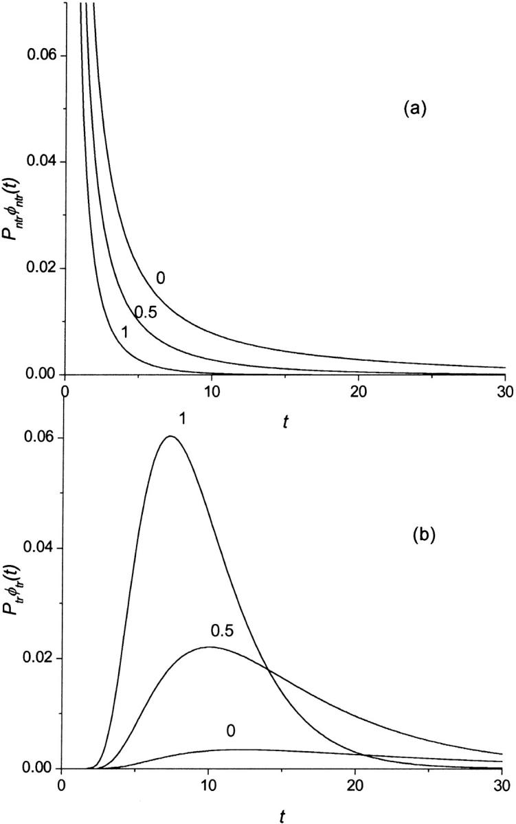
Monotonic (panel a) and nonmonotonic (panel b) components of the probability density  for macromolecules of the contour length
  at different values of the driving force,
  = 0, 0.5, and 1, which are indicated near the curves.
FIGURE 6.

The probability density  (solid curve) and its two components,
  and
and  (dotted and dashed curves) for macromolecules of the contour length
  at the driving force
We have discussed the transition between monotonic and nonmonotonic behavior of the probability density at fixed values of the parameters k and D. In fact, whether φ(t) is monotonic or has two peaks depends on these parameters also. For example, when k → 0 and/or D → ∞, the equilibration occurs much faster than escape and we have
 |
(20) |
and
 |
(21) |
where Γ = kβF coth(βFL/2). One should not be confused by the absence of κ in probabilities given in Eq. 20, which are the leading terms of the probabilities given in Eqs. 15 and 16 in the small κ limit. Additional explanation of the dependence on κ is given just below Eq. 16.
CONCLUDING REMARKS
To analyze the residence time that macromolecules spend in the membrane channel, we have used a one-dimensional diffusion model that is similar to one suggested by Lubensky and Nelson (1999). The key difference between the two models is that we impose radiation (partially and not perfectly absorbing) boundary conditions at the ends of the interval whereas Lubensky and Nelson assumed that the ends are perfectly absorbing. This difference in the boundary conditions is really important because it allowed us to eliminate the “pathology” inherent in the Lubensky-Nelson model.
The translocation probability and Laplace transform of the residence time probability density were derived within the framework of our model. The Laplace transform was numerically inverted to study how the probability density depends on the length of the macromolecule and external driving force. It is interesting that the probability density changes its shape at a certain critical value of the driving force. The density has two peaks when the driving force is larger that the critical value and monotonically decreases with time when the force is smaller that this value. The dependencies predicted by the model in sufficiently strong fields are the same as those observed in experiments on driven translocation of single-stranded RNA and DNA molecules through single α-hemolysin ion channels by Kasianowicz et al. (1996).
The model analyzed in the paper is oversimplified because we assume that the polymer is a rigid rod. Single-stranded DNA and RNA molecules used in the experiment correspond more closely to a freely jointed polymer chain. For such polymers the entropy barrier has to be taken into consideration as first indicated by Sung and Park (1996). Neglecting the entropy potential, we considerably simplify the problem. This makes it possible to derive an exact solution for the Laplace transform of the probability density of the polymer lifetime in the channel, which is used in our analysis to study the shape of the probability density as a function of the driving force and the length of the polymer. It is impossible to find an analytical solution without this simplifying assumption, i.e., when the entropy barrier is included. The fact that our model predicts the behavior qualitatively similar to that observed in the experiment suggests that the contribution into the driving force due to the entropy potential is small compared to the contribution due to the external field when the field is strong enough. We suppose to analyze this question in the future.
Acknowledgments
We thank Sergei Bezrukov and Attila Szabo for very helpful discussions. We also thank P. Valko for his help with the BigNumber-Stehfest algorithm.
A. M. Berezhkovskii's permanent address is Karpov Institute of Physical Chemistry, Moscow 103064, Russia.
I. V. Gopich is on leave from the Institute of Chemical Kinetics and Combustion, Siberian Branch of the Russian Academy of Sciences, Novosibirsk 630090, Russia.
References
- Akeson, M., D. Branton, J. J. Kasianowicz, E. Brandin, and D. W. Deamer. 1999. Microsecond time-scale discrimination among polycytidylic acid, polyadenylic acid, and polyuridylic acid as homopolymers or as segments within single RNA molecules. Biophys. J. 77:3227–3233. [DOI] [PMC free article] [PubMed] [Google Scholar]
- Baumgartner, A., and J. Scolnick. 1994. Polymer electrophoresis across a model membrane. J. Phys. Chem. 98:10655–10658. [Google Scholar]
- Baumgartner, A., and J. Skolnick. 1995. Spontaneous translocation of a polymer across a curved membrane. Phys. Rev. Lett. 74:2142–2145. [DOI] [PubMed] [Google Scholar]
- Bezrukov, S. M., I. Vodyanoy, and V. A. Parsegian. 1994. Counting polymers moving through a single ion channel. Nature. 370:279–281. [DOI] [PubMed] [Google Scholar]
- Bezrukov, S. M. 2000. Ion channels as molecular coulter counters to probe metabolite transport. J. Membr. Biol. 174:1–13. [DOI] [PubMed] [Google Scholar]
- Carl, W. A. 1998. A polymer threading a membrane: model system for a molecular pump. J. Chem. Phys. 108:7921–7922. [Google Scholar]
- Chern, S. S., A. E. Cardenas, and R. D. Coalson. 2001. Three-dimensional dynamic Monte Carlo simulations of driven polymer transport through a hole in a wall. J. Chem. Phys. 115:7772–7782. [Google Scholar]
- Chuang, J., Y. Kantor, and M. Kardar. 2002. Anomalous dynamics of translocation. Phys. Rev. E. 65:118021–118028. [DOI] [PubMed] [Google Scholar]
- De Gennes, P. G. 1999a. Problems of DNA entry into a cell. Physica A. 274:1–7. [Google Scholar]
- De Gennes, P. G. 1999b. Flexible polymers in nanopores. Adv. Polym. Sci. 138:91–105. [Google Scholar]
- De Gennes, P. G. 1999c. Passive entry of a DNA molecule into a small pore. Proc. Natl. Acad. Sci. USA. 96:7262–7264. [DOI] [PMC free article] [PubMed] [Google Scholar]
- Deutsch, J. M., and H. Yoon. 1997. Macromolecular separation through a porous surface. J. Chem. Phys. 106:9376–9381. [Google Scholar]
- Di Marzio, E. A., and A. J. Mandell. 1997. Phase transition behavior of a linear macromolecule threading a membrane. J. Chem. Phys. 107:5510–5514. [Google Scholar]
- Di Marzio, E. A. 1999. The ten classes of polymeric phase transitions: their use as models for self-assembly. Prog. Polym. Sci. 24:329–377. [Google Scholar]
- Han, J., S. W. Turner, and H. G. Craighead. 1999. Entropic trapping and escape of long DNA molecules at submicron size constriction. Phys. Rev. Lett. 83:1688–1691. [Google Scholar]
- Henrickson, S. E., M. Misakian, B. Robertson, and J. J. Kasianowicz. 2000. Driven DNA transport into an asymmetric nanometer-scale pore. Phys. Rev. Lett. 85:3057–3060. [DOI] [PubMed] [Google Scholar]
- Kasianowicz, J. J., E. Brandin, D. Branton, and D. W. Deamer. 1996. Characterization of individual polynucleotide molecules using a membrane channel. Proc. Natl. Acad. Sci. USA. 93:13770–13773. [DOI] [PMC free article] [PubMed] [Google Scholar]
- Kumar, K. K., and K. L. Sebastian. 2000. Adsorption-assisted translocation of a chain molecule through a pore. Phys. Rev. E. 62:7536–7539. [DOI] [PubMed] [Google Scholar]
- Lee, N., and S. Obukhov. 1996. Diffusion of a polymer chain through a thin membrane. J. Phys. II. 6:195–204. [Google Scholar]
- Lubensky, D. K., and D. R. Nelson. 1999. Driven polymer translocation through a narrow pore. Biophys. J. 77:1824–1838. [DOI] [PMC free article] [PubMed] [Google Scholar]
- Meller, A., L. Nivon, and D. Branton. 2001. Voltage-driven DNA translocations through a nanopore. Phys. Rev. Lett. 86:3435343–3435348. [DOI] [PubMed] [Google Scholar]
- Muthukumar, M. 1999. Polymer translocation through a hole. J. Chem. Phys. 111:10371–10374. [Google Scholar]
- Muthukumar, M. 2001. Translocation of a confined polymer through a hole. Phys. Rev. Lett. 86:3188–3191. [DOI] [PubMed] [Google Scholar]
- Park, P. J., and W. Sung. 1998a. A stochastic model of polymer translocation dynamics through biomembranes. Int. J. Bifurcat. Chaos. 8:927–931. [Google Scholar]
- Park, P. J., and W. Sung. 1998b. Polymer release out of a spherical vesicle through a pore. Phys. Rev. E. 57:730–734. [Google Scholar]
- Park, P. J., and W. Sung. 1998c. Polymer translocation induced by adsorption. J. Chem. Phys. 108:3013–3018. [Google Scholar]
- Peskin, C. S., G. M. Odell, and G. F. Oster. 1993. Cellular motions and thermal fluctuations: the Brownian ratchet. Biophys. J. 65:316–324. [DOI] [PMC free article] [PubMed] [Google Scholar]
- Schatz, G., and B. Dobberstein. 1996. Common principles of protein translocation across membranes. Science. 271:1519–1526. [DOI] [PubMed] [Google Scholar]
- Simon, S. M., C. S. Peskin, and G. F. Oster. 1992. What drives the translocation of proteins? Proc. Natl. Acad. Sci. USA. 89:3770–3774. [DOI] [PMC free article] [PubMed] [Google Scholar]
- Stehfest, H. 1970. Algorithm 368: Numerical inversion of Laplace transforms. Comm. ACM. 13:47–49. [Google Scholar]
- Sung, W., and P. J. Park. 1996. Polymer translocation through a pore in a membrane. Phys. Rev. Lett. 77:783–786. [DOI] [PubMed] [Google Scholar]
- Valko, P. P., and S. Vajda. 2002. Inversion of noise-free Laplace transforms: towards a standardized set of test problems. Inverse Problems in Engineering. 10:467–483. (See also http://pumpjack.tamu.edu/∼valko/). [Google Scholar]
- Yoon, H. G., and J. M. Deutsch. 1995. Dynamics of a polymer in the presence of permeable membranes. J. Chem. Phys. 102:9090–9095. [Google Scholar]