Statistical Tests of the Coalescent Model Based on the Haplotype Frequency Distribution and the Number of Segregating Sites

Abstract

Several tests of neutral evolution employ the observed number of segregating sites and properties of the haplotype frequency distribution as summary statistics and use simulations to obtain rejection probabilities. Here we develop a “haplotype configuration test” of neutrality (HCT) based on the full haplotype frequency distribution. To enable exact computation of rejection probabilities for small samples, we derive a recursion under the standard coalescent model for the joint distribution of the haplotype frequencies and the number of segregating sites. For larger samples, we consider simulation-based approaches. The utility of the HCT is demonstrated in simulations of alternative models and in application to data from Drosophila melanogaster.

SELECTIVELY neutral models of within-species evolution consist of a model that describes the genealogy of sampled DNA sequences and a model for the stochastic process of mutation along the branches of the genealogy. Typical neutral models use the coalescent process (Nordborg 2001, for example) to describe the genealogy and the infinitely many sites model (Watterson, 1975) for the mutation process. Many theoretical predictions have been made under the standard neutral model, in which the particular coalescent model chosen is the one with constant population size.

As an alternative to computationally intensive comparisons of likelihoods of DNA sequence data under null and alternative models (Griffiths and Tavaré 1994; Kuhner et al. 1998; Thomson et al. 2000), summaries of variation in a sample of sequences are often used in testing neutral models (Kreitman 2000; Nielsen 2001; Ford 2002). Test statistics computed from the data are compared to theory-based predictions. If such predictions are unavailable or intractable, hypothesis testing is performed using simulations of the appropriate model.

Several neutrality tests use summary statistics based on the frequency distribution of haplotypes in a sample of DNA sequences from a particular region of a genome (Table 1). These “haplotype tests” are sometimes used to detect positive selection on particular haplotypes (Hudson et al. 1994). Alternatively, because haplotype frequency distributions may differ greatly across demographic scenarios (Nei et al. 1975; Donnelly 1996), haplotype tests can also help to identify deviations from the demographic assumptions of the standard neutral model.

TABLE 1.

Haplotype-based tests of the neutral coalescent

Test	Quantity on which test is based	Reference for theoretical predictions about quantity	Reference for test
Ewens-Watterson homozygosity test	P(F|K, n)	Ewens (1972); Watterson (1977)	Watterson (1977)(1978)
Exact test conditional on K	P(C|K, n)	Ewens (1972)	Slatkin (1994)(1996)
Hudson et al. haplotype test   (HHT)	P(M|S, n, θ)	This article	Hudson et al. (1994)
Haplotype no. test (HNT)	P(K|S, n, θ)	Griffiths and Tavaré (1996);   this article	Depaulis and Veuille (1998);   Depaulis et al. (2001);   Markovtsova et al. (2001);   Wall and Hudson (2001)
Haplotype diversity test (HDT)	P(H|S, n, θ)	This article	Depaulis and Veuille (1998);   Depaulis et al. (2001);   Markovtsova et al. (2001);   Wall and Hudson (2001)
Haplotype configuration   test (HCT)	P(C|S, n, θ)	This article	This article

Additional haplotype tests are discussed by Fu (1996, 1997), Kreitman (2000), and Sabeti et al. (2002). Fu (1998) provides a related but not haplotype-based test that uses the configuration of segregating sites in the sample.

Some of the first haplotype tests, such as the Ewens-Watterson homozygosity test, were based on the Ewens (1972) sampling theory for the infinitely many alleles mutation model. Because “allele” in this model and “haplotype” in the infinitely many sites model have the same meaning, the Ewens (1972) theory provides the conditional distribution of the haplotype frequency vector C given the sample size n and the number of distinct haplotypes K, under the standard neutral model (Tavaré and Ewens 1998, Equation 6). In the Ewens-Watterson test, haplotype homozygosity (F) is estimated for a sample of DNA sequences at a nonrecombining locus as the sum of the squares of observed haplotype relative frequencies (Watterson 1977, 1978). Given n, the value of F is compared to the known null distribution, and the neutral model is rejected if F is unusually high or low. A subsequent “exact test” was based on whether C itself was unlikely given n and K (Slatkin 1994, 1996).

Other, more recently devised, haplotype-based tests reject the null hypothesis when the haplotype frequency distribution is unlikely under the same neutral model, given the number of mutations, or segregating sites (S), observed in the data (these tests are also conditioned on a mutation parameter θ, which for now we assume to be known). The adoption of a genealogical perspective has contributed to this shift in emphasis; in neutral models, conditional on the total length (L) of the genealogical tree that underlies the data, E[S|L] is proportional to L (Hudson 1990, for example). Thus, conditioning on S loosely serves as a proxy for conditioning on tree length.

Three main test statistics have been used in haplotype-based tests conditioned on S (Hudson et al. 1994; Depaulis and Veuille 1998): the absolute frequency of the most frequent haplotype (M), the number of distinct haplotypes (K), and the haplotype diversity (H). For each test statistic, many approaches are possible for implementing the test. We term tests based on M, K, and H the Hudson et al. haplotype test (HHT), haplotype number test (HNT), and haplotype diversity test (HDT), respectively, allowing each name to apply to the collection of implementations of the relevant test.

Here we develop a “haplotype configuration test” of neutrality (HCT) conditional on S. This test is analogous to the exact test of Slatkin (1994, 1996), which does not take S into account. The HCT tests if the haplotype frequency vector C is an unlikely configuration, given S (and the mutation parameter θ). The haplotype configuration C conveniently summarizes the pattern of variation among DNA sequences; it perhaps incorporates more information about the data than do M, K, and H, but its use is less cumbersome than full-likelihood inference based on the DNA sequences themselves.

First, we derive a recursion for the joint distribution P(C, S|n, θ), and we show how it can be used to obtain the conditional distribution P(C|S, n, θ). This recursively calculated conditional distribution allows exact computation of rejection probabilities for the HCT for small values of S and n. Because M, K, and H are calculated from C, the recursion can also enable exact computation of rejection probabilities for the HHT, HNT, and HDT. For large S and n, use of the recursion is slow, and we discuss simulation techniques for all four tests. We describe simulation-based extensions that allow for more complex null hypotheses, which may include such phenomena as migration and recombination. We also consider various ways for addressing the problem that θ might not be “known”; in particular we argue that the effect of θ on haplotype tests can be addressed by using prior information about θ from genomic surveys. Finally, we consider the power of the HCT, HHT, HNT, and HDT against alternative models, and we apply the tests to an example from Drosophila melanogaster. The mathematical notation used here is shown in Table 2.

TABLE 2.

Notation

Symbol	Quantity represented
n	Sample size
θ	Mutation parameter (θ = 2Nμ)
N	Haploid population size [or scaling constant for the neutral coalescent model (Nordborg 2001)]
μ	DNA sequence length times mutation rate per base pair per generation
ρ	Recombination parameter (ρ = 2Nr)
r	DNA sequence length times recombination rate per base pair per generation
l	DNA sequence length measured in base pairs
I	No. of segments into which a recombination graph subdivides a DNA sequence
β	Exponential population growth parameter
γ	Migration parameter in the two-island model in which both populations each have size N/2 (γ = 2Nm)
m	In the symmetric two-island model, the fraction of individuals per population who migrate each generation
S	No. of segregating sites
M	Absolute frequency of the most frequent haplotype (that is, the number of sampled copies of the haplotype)
K	No. of haplotypes
H	Haplotype heterozygosity (or haplotype diversity)
F	Haplotype homozygosity (F = 1 − H)
G	A univariate haplotype summary statistic in general (for example, M, K, or H)
Wn	Waiting time until n lineages coalesce to n − 1 lineages
L	Total length of a genealogy with n lineages
C = (C1, … , Cn)	Haplotype frequency vector (or haplotype configuration)
Ck	No. of distinct haplotypes with absolute frequency k
ek	Vector with kth coordinate 1 and other coordinates 0
δi,j	Kronecker's δ (1 if i = j, 0 otherwise)

Corresponding lowercase letters are used for particular instances of random variables.

THEORY

Joint distribution of C and S:

We abbreviate P(C = c, S = s|n, θ) by q(c, s|n, θ). This provides the probability that for n lineages and mutation parameter θ the haplotype configuration is c = (c₁, c₂, … , c_n) and s segregating sites are observed, where c_k is the number of haplotypes with absolute frequency k. We also abbreviate P(C = c|S = s, n, θ) by q(c|s, n, θ) and P(C = c|n, θ) by q(c|n, θ). We wish to express q(c, s|n, θ) in terms of probabilities for states one event backward in time, where an “event” is either a coalescence of two lineages or a mutation. Using the standard neutral coalescent model with population size N (Nordborg 2001, for example) and an infinitely many sites mutation model with mutation parameter θ, time is scaled in units of N generations so that the waiting time until the most recent coalescence is exponentially distributed with rate n(n − 1)/2 and so that for each lineage, the waiting time until a mutation is exponentially distributed with rate θ/2. Because n lineages are present and because mutations on different lineages occur independently of one another, the waiting time (backward in time) until a mutation happens on any lineage is exponentially distributed with rate nθ/2. The probability that the most recent event is a coalescence is (n − 1)/(θ + n − 1), and the probability that it is a mutation is θ/(θ + n − 1), regardless of the time of the event. Suppose the event is a coalescence (a branching, if viewed forward in time). Then for each of k = 1, 2, … , n − 1, it is possible that a haplotype of absolute frequency k + 1 was generated by branching from a haplotype that had frequency k in the previous step. The probability that the event produces a haplotype of frequency k + 1 is the fraction of lineages whose haplotypes had frequency k in the previous step, or k(c_k + 1)/(n − 1).

If the event is a mutation, with probability c₁/n the mutation occurs along a lineage of absolute frequency one, leaving the haplotype configuration unchanged. For each of k = 2, 3, … , n, it is also possible that a lineage whose haplotype has frequency k experiences the mutation. In this situation, which has probability k(c_k + 1)/n, a haplotype of frequency k is replaced by a singleton haplotype and a haplotype of frequency k − 1.

These cases are combined to produce the recursion:

1

In (1), e_k is the n-dimensional vector with the kth coordinate equal to 1 and all other coordinates equal to 0. For convenience, we treat all vectors as having length n, appending extra zeros to the ends of vectors of smaller lengths. We also specify the following rules:

2

3

4

5

6

7

Induction using (1) with (2)–(7) can be used to derive various well-known results, as well as new expressions for n = 3 and n = 4 (Table 3). For larger n, the expression becomes unwieldy and numerical evaluation of (1) at particular θ values is preferable (Table 4).

TABLE 3.

q(c,s|n, θ) in special cases

Configuration (c)	No. of segregating sites (s)	Sample size (n)	q(c, s|n, θ) derived using (1) (by induction on s or n)	Reference for earlier derivation
(0, 1)	0	2		Malécot (1969); Watterson   (1975)
(2, 0)	s ≥ 1	2		Watterson (1975); Tajima (1983)
(0, 0, 1)	0	3		Special case of Ewens (1972)(1974)
(1, 1, 0)	s ≥ 1	3	2θs + −
(3, 0, 0)	s ≥ 2	3	2θs − + + −
(0, 0, 0, 1)	0	4		Special case of Ewens (1972)(1974)
(0, 2, 0, 0)	s ≥ 1	4	+ −
en	0	n		Ewens (1972)(1974)

Expressions for the other three configurations with n = 4 are rather unwieldy and are not shown.

TABLE 4.

Joint probabilities of haplotype configuration and number of segregating sites forn = 5 and θ = 1

Configuration (c)	q(c|n, θ)	q(c, 0|n, θ)	q(c, 1|n, θ)	q(c, 2|n, θ)	q(c, 3|n, θ)	q(c, 4|n, θ)	q(c, 5|n, θ)
(5, 0, 0, 0, 0)	0.0083	0	0	0	0	0.0022	0.0023	0.0039
(3, 1, 0, 0, 0)	0.0833	0	0	0	0.0273	0.0231	0.0147	0.0181
(2, 0, 1, 0, 0)	0.1667	0	0	0.0740	0.0435	0.0235	0.0124	0.0132
(1, 2, 0, 0, 0)	0.1250	0	0	0.0521	0.0334	0.0187	0.0100	0.0108
(1, 0, 0, 1, 0)	0.2500	0	0.1608	0.0482	0.0209	0.0101	0.0050	0.0050
(0, 1, 1, 0, 0)	0.1667	0	0.0958	0.0368	0.0172	0.0085	0.0042	0.0042
(0, 0, 0, 0, 1)	0.2000	0.2000	0	0	0	0	0	0

q(c|n, θ) is given by the Ewens sampling formula (12), and q(c, s|n, θ) is obtained from (1).

Summing (1) from s = 0 to ∞ and rearranging terms produces the following recursion for q(c|n, θ):

8

Conditions associated with (8) are obtained from sums of corresponding conditions for (1) from s = 0 to ∞:

9

10

11

It can be shown that (8) is equivalent to a recursion satisfied by the Ewens (1972) sampling formula and used in its proof (Karlin and McGregor 1972, Equation 9). Thus, the solution to (8) with the initial condition (9) is the Ewens sampling formula (Ewens 1972; Tavaré and Ewens 1998, Equation 3):

12

where θ_(n) = θ(θ + 1) · · · (θ + n − 1), c₁, c₂, … , c_n are nonnegative integers, and . It is straightforward to verify that (12) indeed satisfies (8).

Joint distribution of univariate haplotype summary statistics and S:

The statistics M, K, and H are functions of the frequency vector C as follows:

13

14

15

For a given n, only finitely many haplotype configurations are possible; thus, M, K, and H each have a finite range. The probability that one of these statistics, G, equals a value g, is obtained by summing q(c, s|n, θ) over the configurations that produce the value g:

16

Conditioning on S:

The conditional probability of C, given S, n, and θ, is the quotient of the joint probability of C and S and the probability of observing S segregating sites:

17

The denominator is the sum of the numerator over all configurations and equals

18

(Tavaré 1984, Equation 9.5). Equations similar to (17) apply for M, K, and H; if G represents one of these statistics, then

19

STATISTICAL TESTS

The exact computation of q(c|s, n, θ) suggests the following haplotype configuration test (HCT).

Procedure 1—exact implementation of the haplotype configuration test:

1. Under the null hypothesis of neutrality, use (17) to compute the probabilities of all haplotype configurations, given s, n, and the known θ.

2. Sum the probabilities of all haplotype configurations whose probabilities under the null model are less than or equal to the probability of the observed configuration c. That is, compute

   20

3. Reject the null hypothesis at level α if P ≤ α. Two-tailed haplotype tests based on univariate summary statistics can be implemented in a similar manner (one-tailed versions of these tests are also possible).

Procedure 2—exact implementation of (two-tailed) haplotype tests based on univariate summary statistics:

1. Under the null hypothesis of neutrality, use (19) to compute the probabilities of all possible values of the summary statistic G given s, n, and the known θ.

2. If g denotes the observed value of G in the data, reject the null hypothesis at level α if P(G ≤ g) ≤ α/2 or if P(G ≥ g) ≤ α/2.

For the tests based on M, K, and H, the null hypothesis is rejected if a particular aspect of the observed haplotype frequency distribution is a rare occurrence. Using the HCT, however, the null hypothesis is rejected when the observed haplotype frequency distribution itself is rare. Rare configurations will typically—but not always—have unlikely values for one or more of M, K, and H.

For three choices of θ, Table 5 shows exact probabilities for C, M, K, and H, given s = 10 and n = 7, obtained numerically from (17) and (19). The probabilities shown provide rejection probabilities for the four tests. In Table 5, certain haplotype configurations may be unlikely, even if their values of M, K, and H are centrally located with respect to null distributions of these statistics. For example, (0, 2, 1, 0, 0, 0, 0) is highly unlikely for s = 10 and θ ≈ 4.08: the HCT rejects the null hypothesis at P = 0.0285. However, the frequency of the most frequent haplotype (3), the number of haplotypes (3), and the haplotype diversity (0.6531), are all rather ordinary for the given parameter values.

TABLE 5.

Exact conditional probabilities of haplotype configurations and summary statistics fors = 10,n = 7, and various values of θ, obtained from (17) and (19)

Configuration (c)	q(c|s, n, θ)	Cumulative probability	P[M ≥ M(c)]	P[M ≤ M(c)]	P[K ≤ K(c)]	P[K ≥ K(c)]	P[H ≤ H(c)]	P[H ≥ H(c)]
θ = 1
(7, 0, 0, 0, 0, 0, 0)	0.0058	0.0058	1.0000	0.0058	1.0000	0.0058	1.0000	0.0058
(5, 1, 0, 0, 0, 0, 0)	0.0597	0.2899	0.9942	0.2539	0.9942	0.0655	0.9942	0.0655
(3, 2, 0, 0, 0, 0, 0)	0.1329	0.7891	0.9942	0.2539	0.9345	0.2834	0.9345	0.1985
(1, 3, 0, 0, 0, 0, 0)	0.0554	0.2302	0.9942	0.2539	0.7166	0.6462	0.8015	0.3388
(4, 0, 1, 0, 0, 0, 0)	0.0850	0.4498	0.7462	0.6416	0.9345	0.2834	0.8015	0.3388
(2, 1, 1, 0, 0, 0, 0)	0.2109	1.0000	0.7462	0.6416	0.7166	0.6462	0.6612	0.5497
(0, 2, 1, 0, 0, 0, 0)	0.0408	0.1238	0.7462	0.6416	0.3538	0.9229	0.4503	0.5905
(1, 0, 2, 0, 0, 0, 0)	0.0510	0.1748	0.7462	0.6416	0.3538	0.9229	0.4095	0.7380
(3, 0, 0, 1, 0, 0, 0)	0.0964	0.5462	0.3584	0.8709	0.7166	0.6462	0.4095	0.7380
(1, 1, 0, 1, 0, 0, 0)	0.1099	0.6561	0.3584	0.8709	0.3538	0.9229	0.2620	0.8479
(0, 0, 1, 1, 0, 0, 0)	0.0230	0.0289	0.3584	0.8709	0.0771	1.0000	0.1521	0.8709
(2, 0, 0, 0, 1, 0, 0)	0.0749	0.3648	0.1291	0.9704	0.3538	0.9229	0.1291	0.9459
(0, 1, 0, 0, 1, 0, 0)	0.0246	0.0534	0.1291	0.9704	0.0771	1.0000	0.0541	0.9704
(1, 0, 0, 0, 0, 1, 0)	0.0296	0.0830	0.0296	1.0000	0.0771	1.0000	0.0296	1.0000
θ = 4.08163
(7, 0, 0, 0, 0, 0, 0)	0.0328	0.1113	1.0000	0.0328	1.0000	0.0328	1.0000	0.0328
(5, 1, 0, 0, 0, 0, 0)	0.1877	0.7826	0.9672	0.4818	0.9672	0.2205	0.9672	0.2205
(3, 2, 0, 0, 0, 0, 0)	0.2174	1.0000	0.9672	0.4818	0.7795	0.5812	0.7795	0.4379
(1, 3, 0, 0, 0, 0, 0)	0.0439	0.1975	0.9672	0.4818	0.4188	0.8792	0.5621	0.6251
(4, 0, 1, 0, 0, 0, 0)	0.1433	0.4231	0.5182	0.8310	0.7795	0.5812	0.5621	0.6251
(2, 1, 1, 0, 0, 0, 0)	0.1717	0.5948	0.5182	0.8310	0.4188	0.8792	0.3749	0.7968
(0, 2, 1, 0, 0, 0, 0)	0.0150	0.0285	0.5182	0.8310	0.1208	0.9865	0.2032	0.8118
(1, 0, 2, 0, 0, 0, 0)	0.0192	0.0477	0.5182	0.8310	0.1208	0.9865	0.1882	0.9134
(3, 0, 0, 1, 0, 0, 0)	0.0824	0.2799	0.1690	0.9594	0.4188	0.8792	0.1882	0.9134
(1, 1, 0, 1, 0, 0, 0)	0.0422	0.1536	0.1690	0.9594	0.1208	0.9865	0.0866	0.9556
(0, 0, 1, 1, 0, 0, 0)	0.0037	0.0037	0.1690	0.9594	0.0135	1.0000	0.0444	0.9594
(2, 0, 0, 0, 1, 0, 0)	0.0308	0.0786	0.0406	0.9944	0.1208	0.9865	0.0406	0.9902
(0, 1, 0, 0, 1, 0, 0)	0.0042	0.0079	0.0406	0.9944	0.0135	1.0000	0.0098	0.9944
(1, 0, 0, 0, 0, 1, 0)	0.0056	0.0135	0.0056	1.0000	0.0135	1.0000	0.0056	1.0000
θ = 10
(7, 0, 0, 0, 0, 0, 0)	0.0671	0.2141	1.0000	0.0671	1.0000	0.0671	1.0000	0.0671
(5, 1, 0, 0, 0, 0, 0)	0.2818	1.0000	0.9329	0.6061	0.9329	0.3488	0.9329	0.3488
(3, 2, 0, 0, 0, 0, 0)	0.2269	0.7182	0.9329	0.6061	0.6512	0.7305	0.6512	0.5758
(1, 3, 0, 0, 0, 0, 0)	0.0304	0.0853	0.9329	0.6061	0.2695	0.9450	0.4243	0.7608
(4, 0, 1, 0, 0, 0, 0)	0.1547	0.4913	0.3939	0.8989	0.6512	0.7305	0.4243	0.7608
(2, 1, 1, 0, 0, 0, 0)	0.1225	0.3366	0.3939	0.8989	0.2695	0.9450	0.2392	0.8833
(0, 2, 1, 0, 0, 0, 0)	0.0067	0.0108	0.3939	0.8989	0.0550	0.9959	0.1167	0.8900
(1, 0, 2, 0, 0, 0, 0)	0.0089	0.0197	0.3939	0.8989	0.0550	0.9959	0.1100	0.9606
(3, 0, 0, 1, 0, 0, 0)	0.0617	0.1471	0.1011	0.9816	0.2695	0.9450	0.1100	0.9606
(1, 1, 0, 1, 0, 0, 0)	0.0199	0.0550	0.1011	0.9816	0.0550	0.9959	0.0394	0.9805
(0, 0, 1, 1, 0, 0, 0)	0.0011	0.0011	0.1011	0.9816	0.0041	1.0000	0.0195	0.9816
(2, 0, 0, 0, 1, 0, 0)	0.0154	0.0351	0.0184	0.9982	0.0550	0.9959	0.0184	0.9970
(0, 1, 0, 0, 1, 0, 0)	0.0012	0.0023	0.0184	0.9982	0.0041	1.0000	0.0030	0.9982
(1, 0, 0, 0, 0, 1, 0)	0.0018	0.0041	0.0018	1.0000	0.0041	1.0000	0.0018	1.0000

Cumulative probability refers to the sum of the probabilities of all configurations that have probability at most q(c|s, n, θ). The value θ = 4.08163 was chosen using (26). Unlike θ = 4.08163, the values θ = 1 and θ = 10 are not likely to produce 10 segregating sites.

It is also possible that from among the HHT, HNT, and HDT, one or more tests might reject the null hypothesis at smaller α than does the haplotype configuration test. For example, in Table 5 with θ ≈ 4.08, (7, 0, 0, 0, 0, 0, 0) is unusual at the α = 2 × 0.0328 = 0.0656 level for the HHT, HNT, and HDT, but only at α = 0.1113 using the HCT.

Because C, M, K, and H can take on only finitely many values for a given n, there is some probability that (for example) P(G < g) ≤ α/2 but P(G ≤ g) > α/2. In such cases, procedures 1 and 2 do not reject the null hypothesis and thus are slightly conservative. This situation often arises with small samples, for which not many numbers can be possible values of the test statistics. It occurs most often for M and K, each of which has only n possible values. A small-sample correction for the HCT is to append to step 3 of procedure 1:

if P > α but P − Q < α, where

21

reject the null at level α with probability (α − P + Q)/Q.

For the other tests, we can append to step 2 in procedure 2:

if P(G ≤ g) > α/2 but P(G < g) < α/2, reject the null hypothesis at level α with probability [α/2 − P(G < g)]/P(G = g); if P(G ≥ g) > α/2 but P(G > g) < α/2, reject the null hypothesis at level α with probability [α/2 − P(G > g)]/P(G = g).

Corrections for one-tailed versions of the HHT, HNT, and HDT are analogous. The conservative procedures 1 and 2 are suitable for data analysis; the small-sample correction is most useful when it is important for a rejection region to have fixed size, as in evaluations of the power to reject the null hypothesis under alternative models.

SIMULATION-BASED IMPLEMENTATIONS

Thus far, we have assumed that the sample size and number of segregating sites are small enough that numerical iteration of the recursion is feasible. We have also assumed a simple demographic model without recombination and that θ is known exactly. We now discuss implementations of the HCT and the other tests when these ideal conditions do not hold. First, we consider simulation methods, demographic models, and recombination, continuing to assume that θ is known; we then discuss ways in which uncertainty in θ might be incorporated.

Methods for simulation:

Earlier articles on haplotype tests have described various simulation-based implementations. These algorithms will be generally applicable to the HCT as well. Although exact computation from (17) and (19) is appropriate for small s and n, simulation is necessary as s and n increase.

The procedures that simulate from the correct conditional distribution P(C|S, n, θ) might be classified as Markov chain Monte Carlo methods (Markovtsova et al. 2000, 2001), importance sampling methods (Depaulis et al. 2001), and acceptance-rejection algorithms (Tavaré et al. 1997; Wall and Hudson 2001). A simple and often highly efficient approach is the following version of algorithm 1 of Tavaré et al. (1997).

Procedure 3—acceptance-rejection algorithm for generating samples from P(C|S, n, θ):

1. Simulate the coalescence times W_n, W_n−1, … , W₂ as independent exponentially distributed random variables, with W_j ∼ exp[j(j − 1)/2].

2. Compute the total branch length of the resulting genealogical tree, .

3. Accept the simulated collection of W_j values with probability u, where

   22

   Otherwise, discard the W_j and return to the initial step.

4. Simulate the branching structure of the genealogy by randomly joining lineages until one lineage remains and associate the W_j with corresponding branching events.

5. Independently place S mutations uniformly on the genealogy.

6. Record the haplotype configuration C (and the quantities M, K, and H).

Procedure 3 is then repeated until a prespecified number of genealogies have been accepted. The empirical distribution of C is then used in procedure 1 to decide whether or not to reject the null hypothesis. To implement the HHT, HNT, and HDT, the empirical distributions of M, K, and H are used in the final step of procedure 2.

The efficiency of procedure 3 derives from the fact that it accepts or rejects the simulation before placing S mutations on the branching diagram. It is less efficient to place mutations on the genealogy with a Poisson process with mean Lθ/2 and only afterward accept trees that have accumulated exactly S mutations. The denominator of (22) is the maximum of the numerator over all values of L, ensuring that acceptance will occur reasonably often, except if S is much larger or much smaller than is suggested by the value of θ (Tavaré et al. 1997).

It is noteworthy that even with the efficient algorithm of procedure 3, for large n, due to the large number of possible configurations, the HCT has computational limitations not shared by the other tests. For a given sample size n, the number of possible values of the test statistics for the HHT or HNT is only n. For the HDT, up to a linear transformation, the set of possible values of the statistic is equal to the set of numbers that can equal the sum of the squares of the elements of a partition of n into positive integers (Sloane 2005, entry A069999). The configurations that produce the smallest and largest sums of squares, which equal n and n², respectively, are (n, 0, … , 0) and (0, 0, … , 0, 1). Because the parity of the sum of squares in any partition of n must be the same as that of n, (n² − n + 2)/2 provides an upper bound on the number of possible values of the HDT statistic. Even for sample sizes that are presently considered large, using a large number of accepted simulated genealogies (exceeding the number of possible values of the test statistic by a factor of at least 100), it is feasible to approximate the probabilities of all possible values of M, K, and H.

Unlike the other tests, however, the HCT has the form of an exact test; such tests are characterized by enumeration of the probabilities of all possible data sets under the model and summation of the probabilities of all data sets that are at most as probable as the observed data set (Mehta and Patel 1998). For these tests, the number of possible data sets increases very rapidly with some property of the data (such as the number of alleles at the locus, in exact tests of Hardy-Weinberg proportions). For the HCT, the number of haplotype configurations, equivalent to the number of unordered partitions of n into positive integers, p(n), grows quickly with n (Abramowitz and Stegun 1965, p. 836). While n = 10 has only 42 partitions, n = 50 has 204,226, and there are ∼4 × 10¹² for n = 200. Because enumeration of the probabilities of all configurations is impossible for large samples, the HCT is limited to sample sizes n for which it is feasible to generate at least 100p(n)samples from P(C|S, n, θ). As Markov chain Monte Carlo algorithms have been developed for other exact tests in genetics to avoid the enumeration problem (Guo and Thompson 1992; Raymond and Rousset 1995), it is conceivable that such an algorithm might be developed for this test as well.

Demographic models:

The approach in procedure 3 is versatile, in that the null model need not be the standard constant-size coalescent. A more complex demographic model can be accommodated by substituting its distributions for the waiting times and the branching structure in steps 1 and 4, respectively.

For example, in place of a population with constant size N, consider an exponentially growing population of present population size N with growth parameter β. At t time units of N generations in the past, population size was N exp[−βt]. To use this model as the null, after step 1, for each j, replace W_j by f(W_j), where

23

(Slatkin and Hudson 1991; Nordborg 2001, Equation 8), and for j ∈ {2, 3, … , n − 1},

24

For each j, f(W_j) gives the time to coalescence of j lineages to j − 1, measured in units of N generations. Because variable population size does not change the branching structure of the genealogy, the rest of procedure 3 is identical under exponential population growth.

With a population structure model, such as island migration, as the null, it is simpler to simulate the appropriate waiting times and branching structure concurrently in place of step 1 (Hudson 1990), omitting step 4.

Recombination:

Using the ancestral recombination graph (Hudson 1983; Griffiths and Marjoram 1996; Nordborg 2001), procedure 3 can be extended to allow recombination in the null model. Suppose the recombination parameter for a DNA sequence region is ρ = 2Nr, where l is the number of base pairs in the region and r is l times the recombination rate per base pair per generation. Simulation of the ancestral recombination graph for n lineages consists in repeatedly simulating an exponentially distributed random variable for the time of the next coalescence (appropriately transformed if the model includes population growth) and another exponential random variable for the time of the next recombination. The smaller of the two times gives the type of the next event, which is then allowed to occur, the larger time is discarded, and uniform random variables are simulated to decide which lineages participate in the event. From the graph, a genealogical tree is produced at each base pair, so that nearby base pairs are more likely than distant base pairs to have equivalent trees (Rosenberg and Nordborg 2002, Figure 3, for example). The graph splits the sequence into I segments with lengths l₁, … , l_I, such that all base pairs within a segment have equivalent genealogies, and such that recombination events occur only at segment boundaries. Denote the total branch length of the genealogy of segment i by L_i.

Procedure 4—acceptance-rejection algorithm for generating samples with recombination from P(C|S, n, θ, ρ):

1. Simulate an ancestral recombination graph for n lineages with recombination rate ρ, until all parts of the DNA sequence reach most recent common ancestors.

2. Compute the total branch length of the genealogical tree at an “average” site, .

3. Accept the simulated graph with probability u, where

   25

   Otherwise, discard the graph and return to the initial step.

4. Independently place S mutations uniformly on the genealogy.

5. Record the haplotype configuration C (and the quantities M, K, and H).

This procedure enables haplotype tests to be performed conditional on a known recombination parameter as well as on the known mutation parameter. In the computer program we have implemented, which proceeds more slowly than the algorithm in procedure 4, placement of mutations occurs concurrently with the simulation of the graph in step 1. In place of step 3, the graph is accepted if S mutations are placed, and steps 2 and 4 are omitted.

Treatment of θ:

Because θ does not affect the conditional distribution of C given the sample size and the number of haplotypes, its value is not of concern in neutrality tests based on the Ewens (1972) sampling theory. However, θ does affect P(C|S, n, θ) and analogous distributions for M, K, and H. As an example, in Table 5, for θ = 1, the most common and rarest configurations are (2, 1, 1, 0, 0, 0, 0) and (7, 0, 0, 0, 0, 0, 0), respectively, while (5, 1, 0, 0, 0, 0, 0) is most common and (0, 0, 1, 1, 0, 0, 0) is rarest for θ = 10. Thus, as has been reported for other neutrality tests (Fu 1996, 1998; Markovtsova et al. 2001; Wall and Hudson 2001), it might be expected that the value of θ used can affect rejection probabilities for the HCT, as well as for the HHT, HNT, and HDT.

Table 5 indicates that nominal and actual rejection probabilities for the HCT can differ substantially if the value of θ used is a poor estimate. For example, suppose that the true θ equals 1 and that the configuration (1, 0, 2, 0, 0, 0, 0) is observed with s = 10. The actual HCT rejection probability is P = 0.1748. If no prior knowledge about θ was available, a sensible procedure would be to base P-values on a value of θ estimated using an estimator such as that of Watterson (1975),

26

Equation 26 gives θ̂_W ≈ 4.08; had this estimate been used, it would have been concluded that the observed configuration is significantly unlikely at α = 0.05 (P ≈ 0.0477; see the middle part of Table 5).

This variation in P-values as θ fluctuates suggests that for tests that depend on θ, the standard method for obtaining rejection probabilities when they vary with the unknown value of a nuisance parameter—using the maximal rejection probability across possible values of the parameter (Berger and Boos 1994)—is overly conservative. Indeed, in the example of s = 10 and n = 7, for each of the 14 haplotype configurations possible with s > 0, there is some value of θ for which the configuration is reasonably likely (Figure 1A). In this example, if the largest rejection probability across all values of θ were used, for the HCT, no configuration would lead to rejection at α = 0.05, or even at α = 0.2 (Figure 1B).

Figure 1.—

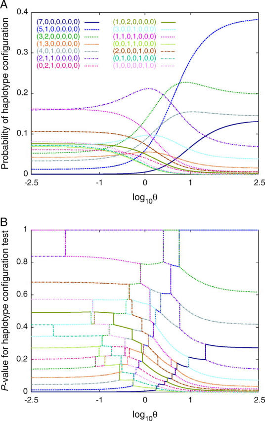
Haplotype configuration test rejection probabilities as functions of θ, for s = 10 and n = 7. (A) Probabilities of haplotype configurations, obtained from (17). (B) P-values for the HCT, obtained from (20). For each value of θ at which two configurations have equal probability—that is, when the curves for the configurations cross in A—HCT P-values for the two configurations both experience discontinuities in θ. In B, data for a given configuration are shown with the same color and pattern as used to depict the configuration in A.

Because point estimates of θ generally have large variances (Felsenstein 1992; Fu and Li 1993), a strategy of maximizing the rejection probability only over a confidence set for θ (Berger and Boos 1994), and not over the full range (0, ∞), is also likely to be quite conservative. This is especially true as P-values can vary considerably in the vicinity of a point estimate (consider Figure 1B at log₁₀θ̂_W ≈ 0.61). Thus, an alternative method is to substitute a distribution of values for θ in a Bayesian procedure (Kelly 1997; Fu 1998; Depaulis et al. 2001). In this scheme, a prior probability density, f_prior(θ), is chosen, and rejection probabilities are evaluated using the density that is proportional to P(C|S, n, θ)f_prior(θ). To implement this approach, we can add a step 0 to procedure 3:

Under exponential growth or recombination, β and ρ can also be chosen from priors, so that evaluation of rejection probabilities is performed conditional on the prior rather than on a fixed growth or recombination rate. Using a uniform prior on [0, 20] for θ (with no growth or recombination), we implemented procedure 3 with s = 10 and n = 7 (Table 6). The distribution for the Bayesian approach is similar to that for θ̂ ≈ 4.08; for the example configuration (1, 0, 2, 0, 0, 0, 0), the HCT rejection probability is 0.0403, close to the value obtained using the point estimate. Other priors, such as uniform distributions on [0, 100] or [0, 500], produce similar results (not shown).

TABLE 6.

Conditional probabilities of haplotype configurations and summary statistics fors = 10 andn = 7, obtained from simulations

Configuration (c)	q(c|s, n, θ)	Cumulative probability	P[M ≥ M(c)]	P[M ≤ M(c)]	P[K ≤ K(c)]	P[K ≥ K(c)]	P[H ≤ H(c)]	P[H ≥ H(c)]
Bayesian approach with a prior of θ ∼ unif[0, 20] (procedure 3)
(7, 0, 0, 0, 0, 0, 0)	0.0437	0.1764	1.0000	0.0437	1.0000	0.0437	1.0000	0.0437
(5, 1, 0, 0, 0, 0, 0)	0.2297	1.0000	0.9563	0.5306	0.9563	0.2734	0.9563	0.2734
(3, 2, 0, 0, 0, 0, 0)	0.2198	0.7703	0.9563	0.5306	0.7266	0.6405	0.7266	0.4932
(1, 3, 0, 0, 0, 0, 0)	0.0374	0.1327	0.9563	0.5306	0.3595	0.9047	0.5068	0.6779
(4, 0, 1, 0, 0, 0, 0)	0.1473	0.3958	0.4694	0.8629	0.7266	0.6405	0.5068	0.6779
(2, 1, 1, 0, 0, 0, 0)	0.1547	0.5505	0.4694	0.8629	0.3595	0.9047	0.3221	0.8326
(0, 2, 1, 0, 0, 0, 0)	0.0144	0.0244	0.4694	0.8629	0.0953	0.9900	0.1674	0.8470
(1, 0, 2, 0, 0, 0, 0)	0.0159	0.0403	0.4694	0.8629	0.0953	0.9900	0.1530	0.9350
(3, 0, 0, 1, 0, 0, 0)	0.0721	0.2485	0.1371	0.9696	0.3595	0.9047	0.1530	0.9350
(1, 1, 0, 1, 0, 0, 0)	0.0319	0.0953	0.1371	0.9696	0.0953	0.9900	0.0650	0.9669
(0, 0, 1, 1, 0, 0, 0)	0.0027	0.0053	0.1371	0.9696	0.0100	1.0000	0.0331	0.9696
(2, 0, 0, 0, 1, 0, 0)	0.0231	0.0634	0.0304	0.9953	0.0953	0.9900	0.0304	0.9927
(0, 1, 0, 0, 1, 0, 0)	0.0026	0.0026	0.0304	0.9953	0.0100	1.0000	0.0073	0.9953
(1, 0, 0, 0, 0, 1, 0)	0.0047	0.0100	0.0047	1.0000	0.0100	1.0000	0.0047	1.0000
Fixed-S approach (Hudson et al. 1994)
(7, 0, 0, 0, 0, 0, 0)	0.0373	0.1216	1.0000	0.0373	1.0000	0.0373	1.0000	0.0373
(5, 1, 0, 0, 0, 0, 0)	0.1951	0.7889	0.9627	0.4852	0.9627	0.2324	0.9627	0.2324
(3, 2, 0, 0, 0, 0, 0)	0.2112	1.0000	0.9627	0.4852	0.7676	0.5838	0.7676	0.4435
(1, 3, 0, 0, 0, 0, 0)	0.0417	0.1633	0.9627	0.4852	0.4162	0.8733	0.5565	0.6254
(4, 0, 1, 0, 0, 0, 0)	0.1402	0.4257	0.5148	0.8292	0.7676	0.5838	0.5565	0.6254
(2, 1, 1, 0, 0, 0, 0)	0.1680	0.5938	0.5148	0.8292	0.4162	0.8733	0.3746	0.7935
(0, 2, 1, 0, 0, 0, 0)	0.0159	0.0322	0.5148	0.8292	0.1267	0.9837	0.2065	0.8094
(1, 0, 2, 0, 0, 0, 0)	0.0198	0.0520	0.5148	0.8292	0.1267	0.9837	0.1906	0.9090
(3, 0, 0, 1, 0, 0, 0)	0.0798	0.2855	0.1708	0.9557	0.4162	0.8733	0.1906	0.9090
(1, 1, 0, 1, 0, 0, 0)	0.0424	0.2057	0.1708	0.9557	0.1267	0.9837	0.0910	0.9514
(0, 0, 1, 1, 0, 0, 0)	0.0043	0.0043	0.1708	0.9557	0.0163	1.0000	0.0486	0.9557
(2, 0, 0, 0, 1, 0, 0)	0.0323	0.0843	0.0443	0.9933	0.1267	0.9837	0.0443	0.9879
(0, 1, 0, 0, 1, 0, 0)	0.0053	0.0096	0.0443	0.9933	0.0163	1.0000	0.0121	0.9933
(1, 0, 0, 0, 0, 1, 0)	0.0067	0.0163	0.0067	1.0000	0.0163	1.0000	0.0067	1.0000

Cumulative probability refers to the sum of the probabilities of all configurations that have probability at most q(c|s, n, θ). For the Bayesian approach, empirical probabilities are based on 10,000 accepted genealogies; for the fixed-S approach, empirical probabilities are based on 10,000 genealogies.

An alternate approach to uncertainty in θ is a simulation strategy that does not explicitly use θ. In this procedure (Hudson 1993; Hudson et al. 1994), equivalent to assuming an implicit density, f_imp(θ|S, n), and simulating from a density proportional to P(C|S, n, θ)f_imp(θ|S, n), the waiting times and branching structures of genealogies are simulated under the neutral coalescent. On each genealogy, S mutations are placed, uniformly and independently. The null distribution of C is taken as the empirical distribution of its values for the simulated trees. If the estimate θ̂_W is close to the true value θ, this procedure produces similar rejection probabilities to both the fixed-θ approach that assumes θ = θ̂_W and the Bayesian procedure in the previous paragraph. However, if θ̂_W and θ differ substantially, the conditional distributions of test statistics by this kind of fixed-S simulation may also be quite different from their conditional distributions given S and θ (Markovtsova et al. 2001; Wall and Hudson 2001). This observation is supported also by our simulation with 10 mutations and n = 7 (Table 6). The probability distribution for fixed-S simulation is quite similar to the exact distribution shown in Table 5 with θ = θ̂_W, and the HCT rejection probability for the example configuration (1, 0, 2, 0, 0, 0, 0) is 0.0520.

Tables 5 and 6 and Figure 1 show that the effect of θ on haplotype tests is not negligible, and that erroneous conclusions might be reached if the observed number of segregating sites is not close to expectation. The problem is not fixed by using a distribution of values for θ estimated from the same data that are to be analyzed using the tests, as such a distribution will likely produce results similar to those obtained with a point estimate. However, the use of diverse regions spread across a genome decreases the variance of an estimate of θ dramatically (Innan et al. 2003). Thus, with genomic polymorphism data, θ can be estimated at many loci independent of the region of interest, and the genomic estimate can be treated as the known value of θ. A collection of values spread around a genomic point estimate might also be used in a Bayesian procedure, although this approach will probably not differ greatly in outcome from use of only the point estimate.

The application of a genomically estimated θ requires the assumption of a constant value of θ across the genome. However, variables such as GC-content and recombination rate may lead to considerable variation in θ (Begun and Aquadro 1992, for example). In such cases, the “known” θ could be estimated within classes of regions that have similar GC-content, levels of recombination, or values of other quantities that influence θ.

POWER

We investigated the power of the four haplotype tests to detect deviations from the standard coalescent model. For various choices of s and n, we used procedure 3 with θ̂_W for θ to obtain the distributions of C, M, K, and H under the null model. For given choices of s and n, the empirical null distributions of C, M, K, and H were based on a set of 10⁶ accepted simulations; for n ≤ 30, this number was found sufficient to ensure that the distributions were accurately estimated. The rejection regions for the tests were defined using procedures 1 and 2, employing simulated probabilities in place of the exact probabilities and using the correction for small sample size: haplotypes on the rejection region boundary for the chosen significance level were assigned an appropriate rejection probability in (0, 1), and all other haplotypes were placed either inside or outside the rejection region.

For each choice of s and n and each alternative model, the power to reject the null for significance level α was equal to the fraction of 10⁵ simulations of the alternative whose haplotypes lay in the α-rejection region. Note that in contrast to the simulations of the null model, which were used to simultaneously estimate a large number of quantities, namely the probabilities of all possible haplotype frequencies or values of a test statistic, simulations of the alternative were used only to estimate what fraction of replicates lay in the rejection region. Thus, in comparison with the null model, to obtain repeatable results, the alternative model required fewer replicates.

Simulations of the alternative model require use of a value of θ. As discussed earlier, when the null hypothesis is true, a sensible choice is to use a value of θ estimated by assuming that the null is true—for example, θ̂_W. Thus, when the alternative hypothesis is true, a sensible choice of θ on which to condition the simulations is a value that would have been estimated assuming that the alternative was true. For a general model in which the expected total branch length of a genealogical tree is E[L], the generalized expression analogous to θ̂_W is 2S/E[L].

In models with recombination, the recombination rate affects the variation across sites in branch lengths of genealogical trees but not the expected total branch length of a randomly chosen site (Pluzhnikov and Donnelly 1996). Thus, the expected total branch length is the same as in the absence of recombination, and consequently we used θ̂_W for the simulations of the alternative model.

For exponential population growth and two-population symmetric island migration models, however, the branch lengths of genealogies differ from those of the standard model. Our simulations of the alternative model employed 2s/ for θ, where was the mean total branch length in 10⁵ simulations of the model. Note that this choice makes the value of θ at which tests were performed dependent on the parameters of the alternative model. Once the value of θ was selected, an independent set of simulations was used for the estimation of power.

Recombination:

If no recombination takes place, the strong correlation of genotypes at neighboring sites makes it fairly likely that if two DNA sequences both contain a mutation at a particular site, they will also share the same haplotype. Thus, many individuals may have the same haplotype, and configurations with high M, low K, and low H are common.

Recombination decouples neighboring sites, so that for large recombination rates, neighboring genotypes are nearly independent. Thus, two sequences with the same genotype at one site will have the same haplotype only if at each of the s − 1 remaining sites they share the same genotype—an unlikely event whose chance of occurring is the product of s − 1 probabilities. Consequently, given s and n, as recombination rate increases, M decreases, K and H increase, and C tends toward configurations that contain many haplotypes of frequency 1, such as se₁ + e_n−s for small s and ne₁ for large s.

For relatively large recombination rates, all tests were able to reject the null model in favor of the recombination model, with power greater in the scenarios with smaller s (Figure 2). For small s, power was comparable for the four tests, whereas for intermediate and large s, the HCT had poorer relative performance than the other tests. The HNT performed particularly well, in agreement with previous observations about the informativeness of K about the recombination rate (Schierup and Hein 2000; Wall 2000; Myers and Griffiths 2003).

Figure 2.—

Power of four tests to reject the standard neutral model at significance level α = 0.05, for three values of s (10, 30, and 75) and three types of alternative models—from top to bottom, recombination, exponential population growth, and island migration. In each plot, n = 30 (in the migration model, the sample was separated into two populations each with sample size 15). Simulation of the null model used procedure 3; simulation of the alternative model used procedure 4 in the case of recombination and appropriately modified versions of procedure 3 in the cases of exponential population growth and island migration (see Demographic models).

Exponential population growth:

Because coalescences are more probable in smaller populations, by increasing the population size in recent generations compared with that of ancient generations, exponential population growth makes it more likely that lineages will persist into the distant past without coalescing. Thus, growth increases lengths of terminal branches of coalescent trees in comparison with those of internal branches. Mutations on terminal branches create single-copy haplotypes, so that growth increases the frequencies of configurations with low M, high K, and high H. As in the recombination case, the configurations se₁ + e_n−s and ne₁ become probable for small and large s, respectively.

In the simulations with exponential growth, the HCT had comparable power to the HNT for small and intermediate s (Figure 2). The HHT and HDT performed rather poorly for small s, improving as s increased. As in the recombination simulations, the HNT was the most generally powerful test. Although some exceptions were observed (for example, with s = 10), similar results were usually obtained when the null hypothesis included recombination (Figure 3).

Figure 3.—

Power of four tests to reject the standard neutral model at significance level α = 0.05 for a null model including recombination (ρ = 10) and two types of alternative models—exponential population growth (top) and island migration (bottom). Simulation of the null model used procedure 4; simulation of the alternative model used appropriately modified versions of procedure 4. The simulations were otherwise the same as in Figure 2.

Island migration:

With a large migration rate, the behavior of the two-population island migration model approaches that of the standard neutral model (Nordborg and Krone 2002, for example). Thus, haplotype frequencies for large migration rates will be similar to those under the null model. As the migration rate decreases, however, lineages coalesce separately in the two populations, with no intervening migrations. The time until one of these lineages migrates to the other population is long, so that genealogies have two long internal branches. These branches contain most mutations, leading to configurations with high M, low K, and low H.

The simulations produced reasonable power with low migration rates and low power with high migration rates (Figure 2). The HCT and HNT had comparable power for intermediate and large s. Similarly to the population growth simulations, the HHT and HDT performed poorly for small s, with similar results when recombination was included in the null hypothesis (Figure 3). As in both the recombination and the growth scenarios, the HNT was the most generally powerful test for small s.

APPLICATION TO DATA

In a data set for the Sod locus in D. melanogaster (Hudson et al. 1994), 55 segregating sites were observed in a sample of size 10, with C = (5, 0, 0, 0, 1, 0, 0, 0, 0, 0). Thus, M = 5, K = 6, and H = 0.7. Using (26), θ̂_W ≈ 19.44. To demonstrate the application of the four haplotype tests, we used procedures 3 and 4 (appropriately modified in the case of exponential population growth) conditional on point estimates for θ (Table 7). For β = 0, the estimate of θ employed (26); for β > 0, the estimate was obtained using simulations, as described in the previous section.

TABLE 7.

Probabilities for data from Hudsonet al. (1994) (×10⁻⁵): c = 5e₁ + e₅,s = 55, andn = 10

		β = 0	β = 0.1	β = 1	β = 10
ρ = 0	C	1699	1442	469	3
M	755	635	222	2
K	5481	4702	1764	50
H	781	647	224	2
ρ = 0.01	C	1722	1394	460	6
M	752	592	230	3
K	5627	4629	1762	46
H	778	612	234	3
ρ = 0.1	C	1776	1381	427	4
M	766	582	217	2
K	5672	4552	1672	52
H	792	602	222	2
ρ = 1	C	1617	1289	368	9
M	726	565	182	4
K	5258	4332	1554	36
H	751	581	182	4
ρ = 10	C	674	540	193	4
M	316	268	97	2
K	2463	2044	795	29
H	320	271	98	2
ρ = 100	C	8	1	0	0
M	3	1	0	0
K	24	12	9	1
	H	3	1	0	0

Values are based on 10⁵ accepted genealogies using a point estimate of θ, estimated from (26) for β = 0 and using 2s/ for β > 0, with based on 10⁵ separate simulated genealogies. If the observed configuration is c, the values in the table are (×10⁵): P(C ≤ c), P[M ≥ M(c)], P[K ≤ K(c)], and P[H ≤ H(c)], where probabilities are estimated from the 10⁵ genealogies. If the observed value of C, M, K, or H was located on the boundary of the rejection region, the null hypothesis was not rejected. To reject the null hypothesis at the 0.05 level, numbers shown must be at most 5000 for the test based on C and 2500 for the other (two-tailed) tests.

As was observed by Hudson et al. (1994), M = 5 is highly unusual under the standard neutral model, as well as under models that include small amounts of population growth and recombination. In each case, the HHT and HDT reject the null hypothesis at very low P-values. The HCT is significant below the 5% level in all cases, while the two-tailed HNT is not significant at the 5% level for low levels of growth and recombination.

CONCLUSIONS

We have introduced the haplotype configuration test of neutrality, which rejects the null hypothesis if the configuration itself is unlikely given S, n, and θ. We have also developed a recursion that allows haplotype tests to be applied exactly for small samples; for larger samples, efficient acceptance-rejection algorithms can be implemented.

Testing the haplotype frequency distribution for anomalies can be viewed as similar to testing if the “site frequency spectrum,” or the distribution of allele frequencies for segregating sites, fits the standard neutral model (Tajima 1989). For the site frequency spectrum, an excess of rare variants can reflect population growth or population structure, whereas an excess of common variants can reflect positive selection or balancing selection. Similarly, conditional on the number of segregating sites, an excess of rare haplotypes may reflect population growth or recombination, while an excess of common haplotypes may reflect population structure or positive selection. As is done for tests based on the site frequency spectrum, the HCT, HHT, HNT, and HDT can be used to scan genomes for atypical regions: for the haplotype tests, to accommodate variability across regions in the number of segregating sites, outlying regions can be identified as those with extreme rejection probabilities (rather than extreme values of the test statistic).

While the HCT perhaps takes into account more information about the data than do the HHT, HNT, and HDT, the various tests reject the null hypothesis under different conditions. The HCT is designed to detect general deviation from the predicted haplotype frequency distribution; although this test may not be optimal for specific alternative scenarios, it may have the potential to identify more diverse departures from the null hypothesis than can be detected with the univariate statistics. Some alternative hypotheses, such as multiallelic balancing selection or positive selection for different haplotypes across subgroups of a structured population, might be better suited to the HCT, as they may be unlikely to produce anomalous values of M, K, or H. For other alternatives, such as positive selection on a single haplotype, univariate statistics such as M may be most appropriate. Regardless of which tests are used, however, genomic data sets will perhaps increase the confidence that can be placed in P-values for haplotype tests and other neutrality tests, because in many species θ will no longer need to be estimated from the same data on which the tests are being performed.

References

- Abramowitz, M. A., and I. A. Stegun, 1965 Handbook of Mathematical Functions. Dover, New York.
- Begun, D. J., and C. F. Aquadro, 1992. Levels of naturally occurring DNA polymorphism correlate with recombination rates in Drosophila melanogaster. Nature 356: 519–520. [DOI] [PubMed] [Google Scholar]
- Berger, R. L., and D. D. Boos, 1994. P values maximized over a confidence set for the nuisance parameter. J. Am. Stat. Assoc. 89: 1012–1016. [Google Scholar]
- Depaulis, F., and M. Veuille, 1998. Neutrality tests based on the distribution of haplotypes under an infinite-site model. Mol. Biol. Evol. 15: 1788–1790. [DOI] [PubMed] [Google Scholar]
- Depaulis, F., S. Mousset and M. Veuille, 2001. Haplotype tests using coalescent simulations conditional on the number of segregating sites. Mol. Biol. Evol. 18: 1136–1138. [DOI] [PubMed] [Google Scholar]
- Donnelly, P., 1996 Variation in the Human Genome, pp. 25–40. Wiley, Chichester, UK.
- Ewens, W. J., 1972. The sampling theory of selectively neutral alleles. Theor. Popul. Biol. 3: 87–112. [DOI] [PubMed] [Google Scholar]
- Ewens, W. J., 1974. A note on the sampling theory for infinite alleles and infinite sites models. Theor. Popul. Biol. 6: 143–148. [DOI] [PubMed] [Google Scholar]
- Felsenstein, J., 1992. Estimating effective population size from samples of sequences: inefficiency of pairwise and segregating sites as compared to phylogenetic estimates. Genet. Res. 59: 139–147. [DOI] [PubMed] [Google Scholar]
- Ford, M. J., 2002. Applications of selective neutrality tests to molecular ecology. Mol. Ecol. 11: 1245–1262. [DOI] [PMC free article] [PubMed] [Google Scholar]
- Fu, Y.-X., 1996. New statistical tests of neutrality for DNA samples from a population. Genetics 143: 557–570. [DOI] [PMC free article] [PubMed] [Google Scholar]
- Fu, Y.-X., 1997. Statistical tests of neutrality of mutations against population growth, hitchhiking and background selection. Genetics 147: 915–925. [DOI] [PMC free article] [PubMed] [Google Scholar]
- Fu, Y.-X., 1998. Probability of a segregating pattern in a sample of DNA sequences. Theor. Popul. Biol. 54: 1–10. [DOI] [PubMed] [Google Scholar]
- Fu, Y.-X., and W.-H. Li, 1993. Maximum likelihood estimation of population parameters. Genetics 134: 1261–1270. [DOI] [PMC free article] [PubMed] [Google Scholar]
- Griffiths, R. C., and P. Marjoram, 1996. Ancestral inference from samples of DNA sequences with recombination. J. Comput. Biol. 3: 479–502. [DOI] [PubMed] [Google Scholar]
- Griffiths, R. C., and S. Tavaré, 1994. Sampling theory for neutral alleles in a varying environment. Philos. Trans. R. Soc. Lond. B 344: 403–410. [DOI] [PubMed] [Google Scholar]
- Griffiths, R. C., and S. Tavaré, 1996. Monte Carlo inference methods in population genetics. Math. Comput. Model. 23: 141–158. [Google Scholar]
- Guo, S. W., and E. A. Thompson, 1992. Performing the exact test of Hardy-Weinberg proportion for multiple alleles. Biometrics 48: 361–372. [PubMed] [Google Scholar]
- Hudson, R. R., 1983. Properties of a neutral allele model with intragenic recombination. Theor. Popul. Biol. 23: 183–201. [DOI] [PubMed] [Google Scholar]
- Hudson, R. R., 1990. Gene genealogies and the coalescent process. Oxf. Surv. Evol. Biol. 7: 1–44. [Google Scholar]
- Hudson, R. R., 1993 The how and why of generating gene genealogies, pp. 23–36 in Mechanisms of Molecular Evolution, edited by N. Takahata and A. G. Clark. Sinauer, Sunderland, MA.
- Hudson, R. R., K. Bailey, D. Skarecky, J. Kwiatowski and F. J. Ayala, 1994. Evidence for positive selection in the superoxide dismutase (Sod) region of Drosophila melanogaster. Genetics 136: 1329–1340. [DOI] [PMC free article] [PubMed] [Google Scholar]
- Innan, H., B. Padhukasahasram and M. Nordborg, 2003. The pattern of polymorphism on human chromosome 21. Genome Res. 13: 1158–1168. [DOI] [PMC free article] [PubMed] [Google Scholar]
- Karlin, S., and J. McGregor, 1972. Addendum to a paper of W. Ewens. Theor. Popul. Biol. 3: 113–116. [DOI] [PubMed] [Google Scholar]
- Kelly, J. K., 1997. A test of neutrality based on interlocus associations. Genetics 146: 1197–1206. [DOI] [PMC free article] [PubMed] [Google Scholar]
- Kreitman, M., 2000. Methods to detect selection in populations with applications to the human. Annu. Rev. Genomics Hum. Genet. 1: 539–559. [DOI] [PubMed] [Google Scholar]
- Kuhner, M. K., J. Yamato and J. Felsenstein, 1998. Maximum likelihood estimation of population growth rates based on the coalescent. Genetics 149: 429–434. [DOI] [PMC free article] [PubMed] [Google Scholar]
- Malécot, G., 1969 The Mathematics of Heredity. W. H. Freeman, San Francisco.
- Markovtsova, L., P. Marjoram and S. Tavaré, 2000. The effects of rate variation on ancestral inference in the coalescent. Genetics 156: 1427–1436. [DOI] [PMC free article] [PubMed] [Google Scholar]
- Markovtsova, L., P. Marjoram and S. Tavaré, 2001. On a test of Depaulis and Veuille. Mol. Biol. Evol. 18: 1132–1133. [DOI] [PubMed] [Google Scholar]
- Mehta, C. R., and N. R. Patel, 1998 Exact inference for categorical data, pp. 1411–1422 in Encyclopedia of Biostatistics, Vol. 2, edited by P. Armitage and T. Colton. Wiley, Chichester, UK.
- Myers, S. R., and R. C. Griffiths, 2003. Bounds on the minimum number of recombination events in a sample history. Genetics 163: 375–394. [DOI] [PMC free article] [PubMed] [Google Scholar]
- Nei, M., T. Maruyama and R. Chakraborty, 1975. The bottleneck effect and genetic variability in populations. Evolution 29: 1–10. [DOI] [PubMed] [Google Scholar]
- Nielsen, R., 2001. Statistical tests of selective neutrality in the age of genomics. Heredity 86: 641–647. [DOI] [PubMed] [Google Scholar]
- Nordborg, M., 2001 Coalescent theory, pp. 179–212 in Handbook of Statistical Genetics, edited by D. J. Balding, M. Bishop and C. Cannings. Wiley, Chichester, UK.
- Nordborg, M., and S. M. Krone, 2002 Separation of time scales and convergence to the coalescent in structured populations, pp. 194–232 in Modern Developments in Theoretical Population Genetics, edited by M. Slatkin and M. Veuille. Oxford University Press, Oxford.
- Pluzhnikov, A., and P. Donnelly, 1996. Optimal sequencing strategies for surveying molecular genetic diversity. Genetics 144: 1247–1262. [DOI] [PMC free article] [PubMed] [Google Scholar]
- Raymond, M., and F. Rousset, 1995. An exact test for population differentiation. Evolution 49: 1280–1283. [DOI] [PubMed] [Google Scholar]
- Rosenberg, N. A., and M. Nordborg, 2002. Genealogical trees, coalescent theory and the analysis of genetic polymorphisms. Nat. Rev. Genet. 3: 380–390. [DOI] [PubMed] [Google Scholar]
- Sabeti, P. C., D. E. Reich, J. M. Higgins, H. Z. P. Levine, D. J. Richter et al., 2002. Detecting recent positive selection in the human genome from haplotype structure. Nature 419: 832–837. [DOI] [PubMed] [Google Scholar]
- Schierup, M. H., and J. Hein, 2000. Consequences of recombination on traditional phylogenetic analysis. Genetics 156: 879–891. [DOI] [PMC free article] [PubMed] [Google Scholar]
- Slatkin, M., 1994. An exact test for neutrality based on the Ewens sampling distribution. Genet. Res. 64: 71–74. [DOI] [PubMed] [Google Scholar]
- Slatkin, M., 1996. A correction to the exact test based on the Ewens sampling distribution. Genet. Res. 68: 259–260. [DOI] [PubMed] [Google Scholar]
- Slatkin, M., and R. R. Hudson, 1991. Pairwise comparisons of mitochondrial DNA sequences in stable and exponentially growing populations. Genetics 129: 555–562. [DOI] [PMC free article] [PubMed] [Google Scholar]
- Sloane, N. J. A., 2005 The On-Line Encyclopedia of Integer Sequences (http://www.research.att.com/~njas/sequences).
- Tajima, F., 1983. Evolutionary relationship of DNA sequences in finite populations. Genetics 105: 437–460. [DOI] [PMC free article] [PubMed] [Google Scholar]
- Tajima, F., 1989. Statistical method for testing the neutral mutation hypothesis by DNA polymorphism. Genetics 123: 585–595. [DOI] [PMC free article] [PubMed] [Google Scholar]
- Tavaré, S., 1984. Line-of-descent and genealogical processes, and their applications in population genetics models. Theor. Popul. Biol. 26: 119–164. [DOI] [PubMed] [Google Scholar]
- Tavaré, S., and W. J. Ewens, 1998 Ewens sampling formula, pp. 230–234 in Encyclopedia of Statistical Sciences Update, Vol. 2, edited by S. Kotz, C. B. Read and D. L. Banks. Wiley, New York.
- Tavaré, S., D. J. Balding, R. C. Griffiths and P. Donnelly, 1997. Inferring coalescence times from DNA sequence data. Genetics 145: 505–518. [DOI] [PMC free article] [PubMed] [Google Scholar]
- Thomson, R., J. K. Pritchard, P. Shen, P. J. Oefner and M. W. Feldman, 2000. Recent common ancestry of human Y chromosomes: evidence from DNA sequence data. Proc. Natl. Acad. Sci. USA 97: 7360–7365. [DOI] [PMC free article] [PubMed] [Google Scholar]
- Wall, J. D., 2000. A comparison of estimators of the population recombination rate. Mol. Biol. Evol. 17: 156–163. [DOI] [PubMed] [Google Scholar]
- Wall, J. D., and R. R. Hudson, 2001. Coalescent simulations and statistical tests of neutrality. Mol. Biol. Evol. 18: 1134–1135. [DOI] [PubMed] [Google Scholar]
- Watterson, G. A., 1975. On the number of segregating sites in genetical models without recombination. Theor. Popul. Biol. 7: 256–276. [DOI] [PubMed] [Google Scholar]
- Watterson, G. A., 1977. Heterosis or neutrality? Genetics 35: 789–814. [DOI] [PMC free article] [PubMed] [Google Scholar]
- Watterson, G. A., 1978. The homozygosity test of neutrality. Genetics 88: 405–417. [DOI] [PMC free article] [PubMed] [Google Scholar]