On the Quantitative Genetics of Mixture Characters

Abstract

Finite mixture models are helpful for uncovering heterogeneity due to hidden structure. Quantitative genetics issues of continuous characters having a finite mixture of Gaussian components as statistical distribution are explored in this article. The partition of variance in a mixture, the covariance between relatives under the supposition of an additive genetic model, and the offspring–parent regression are derived. Formulas for assessing the effect of mass selection operating on a mixture are given. Expressions for the genetic and phenotypic correlations between mixture and Gaussian traits and between two mixture traits are presented. It is found that, if there is heterogeneity in a population at the genetic or environmental level, then genetic parameters based on theory treating distributions as homogeneous can lead to misleading interpretations. Some peculiarities of mixture characters are: heritability depends on the mean values of the component distributions, the offspring–parent regression is nonlinear, and genetic or phenotypic correlations cannot be interpreted devoid of the mixture proportions and of the parameters of the distributions mixed.

FINITE mixture models, used in biology and in genetics since Pearson (1894), are helpful for uncovering heterogeneity due to hidden structure or incorrect assumptions. For instance, unknown loci with major effects can create “bumps” (sometimes quite subtle) in a phenotypic distribution, and this type of heterogeneity may be resolved by fitting a mixture, i.e., by calculating conditional probabilities that a datum is drawn from one of the several potential, yet unknown, genotypes. A brief review of the potential usefulness of mixtures for uncovering major genes is in Lynch and Walsh (1998). Also, many quantitative trait loci detection procedures are based on ideas from mixture models (Haley and Knott 1992).

The quantitative genetics of characters distributed as mixtures has not been studied extensively, although the idea underlies work of, e.g., Latter (1965) and Kimura and Crow (1978). Perhaps this is due to that, until recently, fitting complex hierarchical mixture models to phenotypic data was computationally difficult. However, inference about some quantitative genetic characters via finite mixture models may be warranted in practice. For example, consider mastitis, an inflammation of the mammary gland of cows and goats associated with bacterial infection. The disease affects the dairy industry globally, and it has severe economic effects. Genetic variation in susceptibility to mastitis exists, and selection for increased resistance is feasible (Heringstad et al. 2000). However, recording of mastitis events is not routine in most nations, and milk somatic cell counts (SCC) have been used as a proxy in genetic evaluation of sires (using mixed-effects linear models), because an elevation of SCC is associated with mastitis. It is not obvious how the SCC information should be treated optimally in genetic evaluation. SCC is both an indicator of mastitis and a measure of response to infection. It is reasonable to expect that SCC observations taken on healthy and diseased animals display different distributions, which are “hidden” in the absence of disease recording. Finite mixture models have been suggested in this context by Detilleux and Leroy (2000), Ødegård et al. (2003, 2005), Gianola et al. (2004), and Boettcher et al. (2005).

This article explores quantitative genetics issues of continuous characters having a finite mixture of Gaussian components as statistical distribution. model introduces notation, gives a specification in which both genetic and residual effects follow mixtures, and derives pertinent marginal and conditional distributions. truncation selection gives formulas for assessing the effect of mass selection operating on a mixture. Next, covariance between relatives presents the partition of variance in a mixture, the calculation of covariance between relatives under the supposition of an additive genetic model, and illustrates the effect of heterogeneity on the offspring–parent regression. Genetic and phenotypic correlations between mixture and Gaussian traits, and between two mixture traits, are discussed in covariance structure. This article concludes with some comments and with an appendix, where some basic formulas of mixture distributions are presented.

MODEL

Suppose an observable random variable (y_i, phenotype of individual i) is drawn from the finite mixture of G_E Gaussian components,

(1)

where p_e is a vector containing the mixing proportions (summing to 1); μ_e and are each G_E × 1 vectors of means and variances with typical elements μ_k and , respectively; a_i is the genetic value of i, and denotes a univariate normal density with appropriate mean and variance. As shown in the appendix, the mean and variance of this conditional (given the genetic effect) distribution are

(2)

and

(3)

respectively, where is the residual or “environmental” variance. Informally, is the part of the environmental variance contributed by population heterogeneity.

Assume that the genetic effect a_i is also drawn from the mixture with G_A components

(4)

where , and are the vectors of mixing proportions, component means, and component variances, respectively. Then, , and

(5)

where is the genetic variance, and is interpretable as “variance between genetic means.” In Gaussian linear models the distribution of the random genetic effects is often taken to be N(a_i | 0, ), where is the additive genetic variance, so it may be reasonable to introduce the restriction in the mixture (Verbeke and Lesaffre 1996). The joint density of a_i and y_i is obtained by multiplication of (1) and (4), yielding

(6)

which is a finite mixture of G_E × G_A bivariate normal distributions, with mixing proportion for the kmth component; note that . From standard Gaussian linear models theory, given the km component (let the indicator δ_km = 1 denote such a situation),

where N₂(. | .,.) denotes a bivariate normal distribution. Further,

where

and

Under the standard additive genetic model of Fisher (1918), this regression of “genotype on phenotype” b_km is the heritability of the character under the kmth component of the bivariate mixture. The joint density (6) is also expressible as

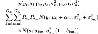(7)

The marginal density of y_i is arrived at by integrating (7) over a_i, yielding

(8)

This is a finite mixture of G_E × G_A univariate normal distributions with mixing proportions . From the appendix, the mean and variance of the phenotypic distribution are

(9)

and

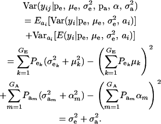(10)

A standard problem in quantitative genetics is that of inferring genetic values from phenotypes. From (7) and (8), the density of the conditional distribution of a_i given y_i is

(11)

where

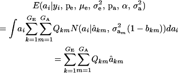
Hence, the conditional distribution of a_i given y_i is a mixture of the G_E × G_A normal distributions , where the mixing proportion is Q_km, the conditional probability that the datum is drawn from , given the observation y_i. The best predictor of genetic value is the conditional expectation function

(12)

(Henderson 1973; Bulmer 1980; Fernando and Gianola 1986; Searle et al. 1992), which is a weighted average of the conditional expectations peculiar to each of the G_E × G_A components of mixture (11). This result is important: the regression of genotype on phenotype is not linear in y_i. Therefore, standard linear models give less than optimal predictions of genetic effects for traits distributed as mixtures. Further, using (39) in the appendix, the variance of the conditional distribution is

(13)

In the standard additive genetic linear model, the variance of the conditional distribution of genotypes given phenotypes is (Falconer 1989), where h² is the coefficient of heritability; this conditional variance is homogeneous and does not depend on the data. In a mixture model, however, the dispersion about the regression function is heteroscedastic and nonlinear on the phenotypic value. Hence, both point and interval predictions of genetic value in mixtures involve strikingly different formulas.

TRUNCATION SELECTION

Consider the standard truncation selection setting in which individuals kept as parents are such that y_i > t, with the proportion of individuals selected being Pr . From (8), the distribution of phenotypic values within selected individuals has density

where

(14)

Above, γ_km is the proportion selected within the kmth mixture component and is the standard normal distribution function. The proportion selected γ is, thus, a weighted average of the individual component selection proportions γ_km. Since the threshold is fixed, the components that are most prevalent, have largest means, and are most variable will be influential.

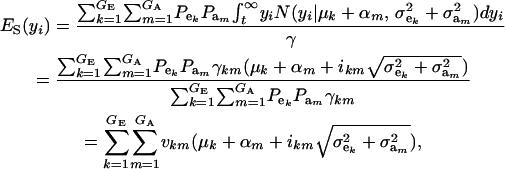
The mean value of selected individuals is

(15)

where i_km is the selection intensity factor under the kmth component (Falconer 1989) and

are relative weights summing to 1. The phenotypic superiority of selected individuals or selection differential is given by the difference between (15) and (9). Further, the mean genetic value of selected parents is

Employing (12),

This expression cannot be evaluated analytically, because it is a highly nonlinear function of the phenotypic values. However, it can be approximated by Monte Carlo procedures, e.g., by drawing samples from the bivariate mixture (7). Accept the draws in which y > t, calculate for each accepted y, and then average this quantity over the samples kept. Finally, the genetic superiority of accepted parents over the unselected population is

The expected fraction of the selection differential that is realized can be assessed as Δ_a/S, and this will differ from what could be expected from the regression of offspring on midparent, because of nonlinearity (see the following section).

Effects of truncation selection upon a heterogeneous population, i.e., a mixture, have been studied extensively in quantitative genetics. For example, Hill (1974) and Bijma and Woolliams (1999) gave formulas for prediction of response suitable for age-structured populations or for overlapping generations. Also, Latter (1965), Lande (1976), and Kimura and Crow (1978) addressed consequences of truncation selection when there is some grouping structure in a population, e.g., caused by genes of large effects. To illustrate, suppose that a genetic mixture derives from a major locus with two alleles. Prior to selection, the mixing proportions (frequencies) of the three genotypes are, in our notation, , and . Also, suppose that the environmental distribution is zero-mean normal, with variance , independent of the genetic distribution, and that the polygenic genetic variance is homoscedastic and equal to (equivalently, the within major genotype genetic variance is constant). Using (14), the overall selection proportion is , and the genotypic frequencies after selection become . After selection, employing (15), the phenotypic distribution has mean value

Falconer (1989) gives approximate expressions for relative fitness of genotypes, e.g., γ₂/γ₁. Note that, under these assumptions, the phenotypic distribution remains a mixture, irrespective of the number of cycles of selection. The means and variance change, however, due to the modification of the frequencies produced by selection.

COVARIANCE BETWEEN RELATIVES

General:

The fraction of variance attributable to additive genetic effects (usual definition of heritability) is location invariant for a Gaussian trait, i.e., it does not involve mean values. In a mixture, “heritability” becomes

(16)

The partition of variance depends on component-specific variances , on mixing proportions ( and ), and on mean values (μ_k and α_m) as well. In the simpler case in which the genetic distribution is the homogeneous process , heritability becomes

(17)

and this is expected to be lower than in a homogeneous population because fixed effects contribute to variance. If the residual variance is homoscedastic across mixture components, this reduces further to

(18)

where . Heterogeneity in means reduces heritability in a mixture , and the standard h² is obtained only when the sampling model invokes a draw from a single component distribution.

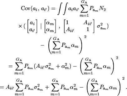
The covariance between phenotypes of related individuals i and i′ is

(19)

after assuming that phenotypes (given the additive genetic values a_i, a_i′) are conditionally independent. To develop the covariance between genetic values further, we assume that these are distributed as the bivariate mixture

where denotes a bivariate normal distribution and A_ii′ is the additive relationship between the two individuals, assumed constant across all components of the mixture; inbreeding is supposed to be nil. It follows directly that each of the genetic values has as marginal distribution. Then

(20)

This reduces to if α_m = 0 for every m and to the standard in the absence of heterogeneity in the distribution of genetic effects.

Regression of offspring on parent:

Using (10) and (20), the standard formula for the regression of the phenotypic value of a progeny (O) on that of a parent (P) (with ) gives

(21)

If the distribution of genetic effects is homogeneous, this simplifies to

(22)

The consequences of (21) and (22) are clear: if there is heterogeneity in the distribution either of sampling model residuals or of genetic effects, then β_OP is affected by the mixing proportions and by the means μ_k. To illustrate, suppose that the genetic distribution is homogeneous; let G_E = 2, take μ₁ = 0 as “origin,” , and . Then (22) is expressible as

When P_e = 1, the formula gives half of heritability, which is a standard result (Falconer 1989). The function is symmetric with respect to P_e; since is maximum at , the regression is minimum at this value. As an example, consider the offspring–parent regression as a function of P_e for four situations with different additive genetic variance () and distances between means (Δ) in the two distributions of the mixture: (1) ; (2) ; (3) ; and (4) . Situations 1 and 2 correspond to a trait with a heritability of 0.50 under homogeneity, while 3 and 4 are for a lowly heritable trait (h² ≈ 0.09). In 1 and 2, the regression β decreases from 0.25 to ∼0.22 and 0.17, respectively, representing relative decreases in heritability of 12 and 32%. The relative decreases in heritability are 18 and 47% in cases 3 and 4, respectively. In brief, heritability in heterogeneous or admixed populations depends on the mixing proportion, on the mean difference between mixture components, and on the “homogeneous situation” heritability.

COVARIANCE STRUCTURE

Correlations with a Gaussian trait:

Correlations between a mixture trait and a normally distributed character may be of interest. For example, the mixture trait could be SCC in dairy cattle, with several component distributions corresponding to different unknown statuses of mammary gland disease. The Gaussian trait could be milk yield of a cow. Is the genetic correlation between the two traits affected by heterogeneity of somatic cell count?

Let the model for the Gaussian trait w be

(23)

where μ_w is the mean of the trait, is the additive genetic value of individual i for trait w, and is a residual effect, independent of a_wi; and are genetic and residual components of variance, respectively. The phenotypic distribution is, thus, .

Suppose that the distribution of mixture trait y has two components at each of the genetic and residual levels; i.e., G_A = G_E = 2. Assume further that

(24)

The distribution of each of the two genetic effects entering into the mixture for trait y (a₁, a₂) is centered at α, but has component-specific variances. These two genetic effects may be imperfectly correlated, with genetic covariance ; for instance, different genes affecting somatic cell count are expressed under the unknown “mastitis” and “no-mastitis” disease conditions generating the mixture. Also, the genetic covariance with the Gaussian trait may be specific to each of the two components. The component-specific residual effects (e₁, e₂) are heteroscedastic but uncorrelated, as it is not possible to observe “disease” and “no disease” in the same individual at the same time. However, a residual correlation with the Gaussian trait is allowed and assumed peculiar to each component distribution.

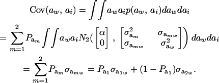
Recall from (4) that . Now, let ∂_m take the value 1 when the draw is from component m and 0 otherwise. The joint density under m is

so that, unconditionally

Then

(25)

Using (5) and (25), and taking α = 0, the genetic correlation between the mixture-distributed trait and the Gaussian character is

(26)

This reduces to the standard when the distribution of genetic effects for trait y is homogeneous and to

(27)

when .

The effect of on genetic correlation (27) is illustrated next. Let be a heteroscedasticity factor, where , the genetic variance under the first component of the mixture, is viewed as “baseline” genetic variance, i.e., a measure of variability in the absence of heterogeneity. Then

(28)

where ρ_homo is the genetic correlation in the absence of a mixture and

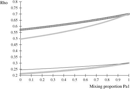
is the factor by which ρ_homo is modified by heterogeneity. Since the sign of is invariant with respect to , it suffices to examine function (28) only under positive values of ρ_homo. Figure 1 displays the relationship between the genetic correlation (28) and for two values of ρ_homo (0.7 and 0.3) and of λ (1.5 and 2). As increases, the proportion of the component with larger genetic variance (m = 2) decreases. The genetic correlation increases monotonically with and more rapidly so at the largest value of genetic heteroscedasticity. Suppose that w is total lactation milk yield in dairy cows and that y is SCC, a mixture trait resulting from the fact that some cows have mastitis (∼20–40%). There is evidence (e.g., Heringstad et al. 2006) that the genetic variance of somatic cell count is ∼2.5 times larger in healthy than in diseased (clinical cases) cows. Under the assumptions leading to (28), our model predicts that the genetic correlation between milk yield and somatic cell score would decrease as the frequency of mastitis in the population decreases. Similar algebra and considerations hold for the environmental correlation between traits.

Figure 1.—

Genetic correlation (Rho) between a Gaussian character and a mixture trait for a two-component mixture, as a function of the mixing proportion (), for different combinations of ρ_homo, genetic correlation in absence of mixture, and λ, heteroscedasticity factor. From top to bottom: (1) ρ_homo = 0.7, λ = 1.5 (open squares); (2) ρ_homo = 0.7, λ = 2 (dotted line); (3) ρ_homo = 0.3, λ = 1.5 (solid line); (4) ρ_homo = 0.3, λ = 2 (open circles).

Consider again the joint distribution (24), and write

(29)

where the random variable δ_e takes the value 1 or 0 with probabilities P_e and 1 − P_e, respectively; δ_a is another binary variable taking the values 1 or 0 with probabilities P_a and (1 −P_a), respectively, and distributed independently of δ_e. These two binary variates are assumed to be independent of a_wi and e_wi entering into the model for w_i in (23). Then,

and

The phenotypic covariance between y and w is, therefore,

Since the second term is null

(30)

Above, is the genetic covariance, as in (25), and is the residual covariance. Collecting (30), (10), plus the fact that , and assuming that α = 0, yields as phenotypic correlation

(31)

The phenotypic correlation depends not only on the underlying components of variance and covariance, but also on the mixing proportions and population means.

If the genetic distribution is homoscedastic , and heterogeneity is at the level of the sampling model only, but with and , the phenotypic correlation becomes

(32)

where is the phenotypic correlation in the absence of a mixture for the residual distribution and . To illustrate, take μ₁ = 0 as origin, μ₂ = Δ, and σ_y = 1. Then

(33)

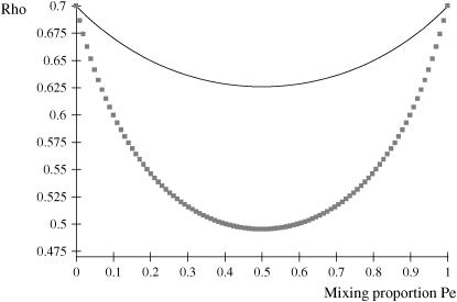
The phenotypic correlation has a minimum at P_e = 0.5 if ρ_homo is positive; however, it is maximum at this value of the mixing proportion if ρ_homo is negative. Effects of P_e and of Δ on the genetic correlation are shown in Figure 2, for ρ_homo = 0.7 and Δ = 1 and 2. The function is symmetric and steeper as Δ increases. For Δ = 2, the correlation decreases from 0.7 (for P_e = 0 or 1) to a minimum of ∼0.50. The curves are inverted if ρ_homo is negative. In short, if the value of is used to measure admixture in the residual distribution, the phenotypic correlation decreases with admixture if it is positive in a homogeneous population. On the other hand, ρ_yw increases with admixture if negative under the homogeneous situation.

Figure 2.—

Phenotypic correlation (Rho) between a Gaussian character and a mixture trait for a two-component mixture, as a function of the mixing proportion (P_e). (1) ρ_homo = 0.7, Δ = 1 (solid line); (2) ρ_homo = 0.7, Δ = 2 (line with squares). ρ_homo, phenotypic correlation in the absence of a mixture; Δ, difference between means of the two distributions.

Correlations between two mixture-distributed characters:

Suppose now that measurements are available for traits y and z. For simplicity, it is assumed that the joint distribution of y and z arises from a two-component mixture of bivariate normal distributions at the level of the sampling model (that is, given the genetic effects) and from a two-component bivariate normal mixture of genetic effects. Given the independently distributed binary indicator variables δ_e and δ_a, one can write

(34)

Then

(35)

Assuming independence between genetic and environmental effects in the distributions, it follows that

where and are the additive and environmental components of covariance between y and z under m, and and are potential cross-mixture covariances. Further, under the assumption of a null mean of the component-specific genetic and environmental distributions, as well as of independence of the binary indicator variables δ_e and δ_a,

and

Since δ_e and δ_a are Bernoulli, , , , and . Then

and

Employing the preceding results in (35),

(36)

Under the assumption that the underlying genetic distributions have zero means, the genetic correlation between the two mixture traits is

The environmental correlation takes the form

and the phenotypic correlation follows from (36) and (10), after setting all α's to 0.

CONCLUSION

Some basic results of standard theory of quantitative genetics under additive inheritance were extended to finite mixture models with Gaussian components. It was found that, if there is heterogeneity in a population at either the genetic or the environmental levels, then genetic parameters based on theory treating distributions as homogeneous can lead to misleading interpretations. Some peculiarities of mixture characters are: heritability depends on the mean values of the populations, the offspring–parent regression is nonlinear, and genetic or phenotypic correlations cannot be interpreted devoid of the mixture proportions and of the parameters of the component distributions. For example, nonlinearity of the offspring–parent regression was studied by Robertson (1977) and Gimelfarb (1986) under dominance and by Im and Gianola (1988) for binary traits. Gimelfarb (1986) gave conditions under which the regression would be nearly linear under dominance, e.g., a large number of loci affecting the trait or mild dominance and gene frequencies not far from 0.5. Our results illustrate that nonlinearity can also arise due to heterogeneity at the environmental level due to, for instance, omitting relevant covariates in a linear model for quantitative genetic analysis.

Clearly, standard models for quantitative traits can lead to erroneous results if fitted to heterogeneous data. If a mixture is suspected, two suitable methods for inferring unknown mixture parameters are maximum-likelihood and Bayesian analyses. Procedures for likelihood- or posterior-based inference applied to mixtures are discussed extensively in Titterington et al. (1985) and McLachlan and Peel (2000), including situations in which the component distributions are not normal, e.g., skewed survival processes. Implementations suitable for fitting different types of quantitative genetic mixture models have been described and applied by Ødegård et al. (2003, 2005), Gianola et al. (2004), and Boettcher et al. (2005). Prediction of breeding values is discussed in Gianola (2005). A suitable software for the analysis of mixtures with random effects is available in a forthcoming update of Version 6.0 of the DMU package (Madsen and Jensen 2002).

An important issue is how many components should be fitted in a mixture model. Testing for the number of components is a difficult matter, and there may not be a one-to-one correspondence between the number of components fitted and the number of heterogeneous groups (McLachlan and Peel 2000). For example, several groups may be hidden behind an apparently bimodal distrbution, due to limited sample size. Also, if some of the component distributions are skewed, typically the number of components needed for a good fit is larger than the number of groups causing heterogeneity. Probably the most elegant procedures for inferring the number of components needed are Bayesian implementations via the reversible-jump algorithm (Richardson and Green 1997), but computations can be extremely taxing.

APPENDIX

The first and second moments, and the variance of a finite mixture of K Gaussian distributions, with parameters , where the mixture proportions P_k are such that , are

(A1)

(A2)

and

(A3)

The first term in (A3) can be interpreted as an average variance, while measures dispersion between group means or heterogeneity; if the μ's are equal, this term is null. The variance of the mixture depends not only on individual component variances, but also on group means. If the components have homogeneous variance σ²,

(A4)

References

- Bijma, P., and J. A. Woolliams, 1999. Prediction of genetic contributions and generation intervals in populations with overlapping generations under selection. Genetics 151: 1197–1210. [DOI] [PMC free article] [PubMed] [Google Scholar]
- Boettcher, P. J., P. Moroni, G. Pisoni and D. Gianola, 2005. Application of a finite mixture model to somatic cell scores of Italian goats. J. Dairy Sci. 88: 2209–2216. [DOI] [PubMed] [Google Scholar]
- Bulmer, M. G., 1980. The Mathematical Theory of Quantitative Genetics. Clarendon Press, Oxford.
- Detilleux, J., and P. L. Leroy, 2000. Application of a mixed normal mixture model to the estimation of mastitis-related parameters. J. Dairy Sci. 83: 2341–2349. [DOI] [PubMed] [Google Scholar]
- Fernando, R. L., and D. Gianola, 1986. Optimal properties of the conditional mean as a selection criterion. Theor. Appl. Genet. 72: 822–825. [DOI] [PubMed] [Google Scholar]
- Gianola, D., 2005. Prediction of random effects in finite mixture models with Gaussian components. J. Anim. Breed. Genet. 122: 145–160. [DOI] [PubMed] [Google Scholar]
- Gianola, D., J. Ødegård, B. Heringstad, G. Klemetsdal, D. Sorensen et al., 2004. Mixture model for inferring susceptibility to mastitis in dairy cattle: a procedure for likelihood-based inference. Genet. Sel. Evol. 36: 3–27. [DOI] [PMC free article] [PubMed] [Google Scholar]
- Falconer, D. S., 1989. Introduction to Quantitative Genetics. Longman, Burnt Mill, Harlow, UK.
- Fisher, R. A., 1918. The correlation between relatives on the supposition of Mendelian inheritance. Trans. R. Soc. Edinb. 52: 399–433. [Google Scholar]
- Gimelfarb, A., 1986. Offspring-parent regression: How linear is it? Biometrics 42: 67–71. [PubMed] [Google Scholar]
- Haley, C. S., and S. A. Knott, 1992. A simple regression method for mapping quantitative trait loci in line crosses using flanking markers. Heredity 69: 315–324. [DOI] [PubMed] [Google Scholar]
- Henderson, C. R., 1973. Sire evaluation and genetic trends, pp. 10–41 in Proceedings of the Animal Breeding and Genetics Symposium in Honor of Dr. Jay L. Lush. American Society of Animal Science and American Dairy Science Association, Champaign, IL.
- Heringstad, B., G. Klemetsdal and J. Ruane, 2000. Selection for mastitis resistance in dairy cattle: a review with focus on the situation in the Nordic countries. Livest. Prod. Sci. 64: 95–106. [Google Scholar]
- Heringstad, B., D. Gianola, Y. M. Chang, J. Ødegård and G. Klemetsdal, 2006. Genetic associations between clinical mastitis and somatic cell score in early first lactation cows. J. Dairy Sci. 89: 2236–2244. [DOI] [PubMed] [Google Scholar]
- Hill, W. G., 1974. Prediction and evaluation of response to selection with overlapping generations. Anim. Prod. 18: 117–139. [Google Scholar]
- Im, S., and D. Gianola, 1988. Offspring-parent regression for a binary trait. Theor. Appl. Genet. 75: 720–722. [Google Scholar]
- Kimura, M., and J. F. Crow, 1978. Effect of overall phenotypic selection on genetic change at individual loci. Proc. Natl. Acad. Sci. USA 75: 6168–6171. [DOI] [PMC free article] [PubMed] [Google Scholar]
- Lande, R., 1976. Natural selection and random genetic drift in phenotypic evolution. Evolution 30: 314–334. [DOI] [PubMed] [Google Scholar]
- Latter, B. D. H., 1965. The response to artificial selection due to autosomal genes of large effect. Aust. J. Biol. Sci. 18: 585–598. [DOI] [PubMed] [Google Scholar]
- Lynch, M., and B. Walsh, 1998. Genetics and Analysis of Quantitative Traits. Sinauer, Sunderland, MA.
- Madsen, P., and J. Jensen, 2002. A User's Guide to DMU. A Package for Analysing Mixed Models, Version 6, Release 4.3. Danish Institute of Agricultural Sciences, Tjele, Denmark.
- McLachlan, G., and D. Peel, 2000. Finite Mixture Models. Wiley, New York.
- Ødegård, J., J. Jensen, P. Madsen, D. Gianola, G. Klemetsdal et al., 2003. Mixture models for detection of mastitis in dairy cattle using test-day somatic cell scores: a Bayesian approach via Gibbs sampling. J. Dairy Sci. 86: 3694–3703. [DOI] [PubMed] [Google Scholar]
- Ødegård, J., P. Madsen, D. Gianola, G. Klemetsdal, J. Jensen et al., 2005. A Bayesian threshold-normal mixture model for analysis of a continuous mastitis-related trait. J. Dairy Sci. 88: 2652–2659. [DOI] [PubMed] [Google Scholar]
- Pearson, K., 1894. Contributions to the mathematical theory of evolution. Philos. Trans. R. Soc. A 185: 71–110. [Google Scholar]
- Richardson, S., and P. J. Green, 1997. On Bayesian analysis of mixtures with an unknown number of components (with discussion). J. R. Stat. Soc. B 59: 731–792. [Google Scholar]
- Robertson, A., 1977. The non-linearity of offspring-parent regression, pp. 297–303 in Proceedings of the International Conference on Quantitative Genetics, edited by E. Pollak, O. Kempthorne and T. B. Bailey, Jr. Iowa State University Press, Ames, IA.
- Searle, S. R., G. Casella and C. E. McCulloch, 1992. Variance Components. Wiley, New York.
- Titterington, D. M., A. F. M. Smith and U. E. Makov, 1985. Statistical Analysis of Finite Mixture Distributions. Wiley, Chichester, UK.
- Verbeke, G., and E. Lesaffre, 1996. A linear mixed effects model with heterogeneity in the random-effects population. J. Am. Stat. Assoc. 91: 217–221. [Google Scholar]