Plant domestication, a unique opportunity to identify the genetic basis of adaptation

Abstract

Despite the fundamental role of plant domestication in human history and the critical importance of a relatively small number of crop plants to modern societies, we still know little about adaptation under domestication. Here we focus on efforts to identify the genes responsible for adaptation to domestication. We start from a historical perspective, arguing that Darwin's conceptualization of domestication and unconscious selection provides valuable insight into the evolutionary history of crops and also provides a framework to evaluate modern methods used to decipher the genetic mechanisms underlying phenotypic change. We then review these methods, framing the discussion in terms of the phenotype–genotype hierarchy. Top-down approaches, such as quantitative trait locus and linkage disequilibrium mapping, start with a phenotype of interest and use genetic analysis to identify candidate genes. Bottom-up approaches, alternatively, use population genetic analyses to identify potentially adaptive genes and then rely on standard bioinformatics and reverse genetic tools to connect selected genes to a phenotype. We discuss the successes, advantages, and challenges of each, but we conclude that bottom-up approaches to understanding domestication as an adaptive process hold greater promise both for the study of adaptation and as a means to identify genes that contribute to agronomically important traits.

Plant domestication fundamentally altered the course of human history. The adaptation of plants to cultivation was vital to the shift from hunter–gatherer to agricultural societies, and it stimulated the rise of cities and modern civilization. Humans still rely on crops that were domesticated >10,000 years ago in such diverse places as Central America, New Guinea, and the Fertile Crescent. Nonetheless, modern humans are reliant on a surprisingly small number of crops: Nearly 70% of the calories consumed by humans are supplied by only 15 crops (Table 1). The cereals are particularly important, with five crops (rice, wheat, maize, sugarcane, and barley) contributing more than half of the calories consumed.

Table 1.

Major world crops ranked by metric tonnage

Rank by tonnage*	Common name	Rank by calories consumed*	Ploidy	Propagation	Life history
1	Sugarcane	4	8×	O, V	P
2	Maize	3	2×	O	A
3	Wheat	2	6×	O	A
4	Rice	1	2×	S	A
5	Potatoes	6	4×	O, V	AP
6	Sugar beet	8	2×	O	A
7	Soybeans	5	2×	S	A
8	Cassava	9	4×	O, V	AP
9	Palm kernel	7	2×	O	P
10	Barley	11	2×	S	A
11	Sweet potatoes	15	4–6×	O, V	AP
12	Tomatoes	30	2×	S	A
13	Watermelons	38	2×	O	A
14	Bananas	19	3×	V	P
15	Brassicas	37	2×	O	A

O, outcrossing; S, selfing; V, vegetative; P, perennial; A, annual; AP, perennial species generally cultivated as annuals.

*Data are from the Food and Agriculture Organization of the United Nations (www.fao.org, 2004).

Despite the critical importance of these crops, in most cases little is known about their domestication. Some obvious questions pertain to the domesticators: Who were they? How did they identify the incipient crop? What were their cultivation methods? Other questions concern crop history: What was the wild progenitor of the modern crop? Did domestication occur more than once? If so, where? The application of phylogeographic methods is beginning to inform the answers to this latter set of questions (1, 2), but the picture for any one crop remains far from complete.

In this article we focus on a third set of questions that revolve around the phenotypic changes associated with domestication. The first question is whether phenotypic changes driven by artificial selection are an apt analogy for adaptation in nature. We take a historical perspective on this issue, arguing that Darwin's conceptualization of domestication provides valuable insight into our view of crop history and provides a framework for evaluating methods used to decipher the genetic mechanisms underlying phenotypic change. We then review these methods, framing the discussion in terms of the phenotype–genotype hierarchy, evaluating both “top-down” and “bottom-up” approaches. We conclude by arguing that an appreciation of domestication as an adaptive process has the potential to reveal far more about the genes contributing to agronomic traits than has been learned to date.

Is Artificial Selection Analogous to Natural Selection? A Historical Perspective

In the opening chapter of the Origin of Species, Charles Darwin introduced the idea of natural selection with an analogy to domestication (3). The importance of domestication to Darwin's thinking is evident even in early sketches of his work (4), and Darwin himself claimed that the example of domestication was fundamental to the formulation of his theory (refs. 3, 5, and 6; for a different perspective see ref. 7). But for Darwin domestication was more than a useful analogy: he saw it as a model of adaptation from which inferences about the nature of variation and selection in natural systems could be drawn (7, 8).

Darwin's assertion of the importance of domestication in understanding the evolutionary process was not universally accepted, however. One of the most vocal critics of Darwin's views on domestication was Alfred Russell Wallace. Even in their joint publication announcing the theory of natural selection, Wallace denies the relevance of domestication: “We see, then, that no inferences as to varieties in a state of nature can be deduced from the observation of those occurring among domestic animals” (9). “It has always been considered a weakness in Darwin's work,” he later writes, “that he based his theory, primarily, on the evidence of variation in domesticated animals and cultivated plants” (10).

Wallace found fault with two aspects of domestication as a heuristic for understanding adaptation in nature. He argued first that the analogy was flawed: artificial selection requires an intelligent selector, whereas no such force acts in natural systems. Additionally, he insisted that the selection itself was fundamentally different, leading to intrinsically different kinds of variation. Domesticated species, he wrote, “are abnormal, irregular, artificial; they are subject to varieties which never occur and never can occur in a state of nature: their very existence depends altogether on human care; so far are many of them removed from that just proportion of faculties, that true balance of organization, by means of which alone an animal left to its own resources can preserve its existence and continue its race” (9).

Both of Wallace's lines of argument find modern audiences, from those who see a fundamental difference between the conscious selection of humans and natural processes (11) to those who argue that variation in domesticated species differs from that in nature (12). Yet Darwin directly addressed these ideas with his explicit recognition of unconscious selection (4). Darwin (5) divided human-mediated selection into two components: methodical selection, “systematically endeavor[ing] to modify a breed according to some predetermined standard,” and unconscious selection, “that which follows from men naturally preserving the most valued and destroying the less valued individuals, without any thought of altering the breed.” Unconscious selection, he posited, was no different from natural selection. Humans change the conditions in which cultivated species live and reproduce, and this change exerts selection on the population even in the absence of a choice or predetermined goal by the cultivator.

Although the term “unconscious selection” fell out of use for many years (13), students of crop evolution nonetheless recognized its fundamental role in domestication. Both Vavilov (14) and Engelbrecht (15) viewed the initial stages of domestication as determined entirely by unconscious selection, and modern workers widely cite the central role of unconscious selection, sometimes referred to as automatic (16) or unintentional (17), in effecting observed variation in domesticated species. These authors argue that many of the phenotypic changes associated with domestication are likely to have arisen via unconscious selection and, like Darwin, view unconscious selection, and much of the process of domestication, as illustrative of the process and effects of natural selection.

The phenotypic changes associated with adaptation under domestication are substantial. Many of these changes are shared across a broad array of domesticated plants; this suite of changes is commonly referred to as the “domestication syndrome” (18). Common features of the domestication syndrome are larger fruit or grain, reduced branching, gigantism, the loss or reduction of seed dispersal, the loss of seed dormancy, changes in photoperiod sensitivity, and the loss or reduction of toxic compounds (18, 19). For example, the major cereal crops in Table 1 (rice, wheat, maize, and barley) all experienced a series of parallel phenotypic shifts brought about by domestication, including reduced seed dispersal, reduced branching or tillering, decreased seed dormancy, synchronized seed maturation, an increase in grain size, and larger inflorescences.

We emphasize three salient points about the phenotypic changes associated with domestication. First, with the possible exception of characteristics such as color or fruit size that were clearly desirable by humans, most features of the domestication syndrome are likely the result of unconscious selection (refs. 16, 18, and 20; for a more inclusive view see ref. 5). Second, the traits most clearly resulting from unconscious selection are those that would have been difficult for early cultivators to notice or that would have changed without any direct effort. Seed dormancy, for example, would be selected against by almost any method of cultivation, even without a conscious decision to plant only nondormant individuals. Finally, like its natural counterpart, unconscious selection is not limited to visible phenotypes; much of the adaptation under domestication may have involved physiological or developmental changes corresponding to the new edaphic, photosynthetic, hydrological, and competitive regimes associated with cultivation.

Two Approaches to Finding Adaptive Genes

Dramatic shifts in phenotype associated with domestication are not only important as evolutionary examples; they have broad economic and societal consequences. There is substantial interest in discovering the genes and genetic mechanisms that contribute to phenotypic changes associated with domestication, because their identification may facilitate trait manipulation through modified breeding strategies (21). We discuss two approaches to this goal, starting at opposite ends of the phenotype–genotype hierarchy. To date, most research has followed what we call a top-down approach, which begins with a phenotype of interest and then identifies causative genomic regions via genetic analyses such as quantitative trait locus (QTL) and linkage disequilibrium (LD) mapping (Fig. 1Left). An alternative approach is to build on Darwin's view of domestication, starting with the concept of adaptation and moving from the bottom up. In this approach, population genetic methods are used to search for the signal of adaptation in a set of genes, and traditional molecular methods are used to move from gene to phenotype (Fig. 1 Right). Here we introduce each of these approaches, discuss the methodologies available for their implementation, and assess their strengths and weaknesses.

Fig. 1.

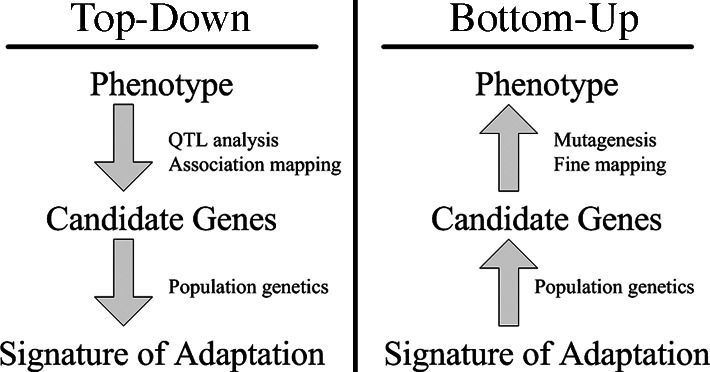
Schematic of the phenotype–genotype hierarchy as represented by top-down and bottom-up approaches.

From the Top Down: QTL and LD Mapping

To date, all of the successes at identifying genes underlying the adaptive changes during domestication have originated from top-down approaches, beginning with the phenotype and using genetic analyses to uncover genomic regions and eventually candidate genes responsible for the phenotype of interest. The most successful method for finding these genes has been QTL mapping, but association or LD methods are rapidly gaining favor in the plant genomics community. While it is beyond the scope of this article to provide a comprehensive review of QTL and LD mapping, we review some empirical findings and highlight some of the challenges of spanning the gap between phenotype and genotype.

QTL Mapping.

Given a trait of interest, QTL mapping was the first (and is still the most widely used) method available for localizing the genetic basis of a trait (e.g., ref. 22). QTL mapping has led to all of the major successes in the identification and cloning of genes underlying domestication traits (23). The best-known examples come from tomato and maize. In the mid-1980s Tanksley and coworkers (24) initiated QTL analysis of fruit mass in a cross between wild and domesticated tomato, localizing six QTLs. With extensive mapping efforts, they were able to isolate a region encompassing the major QTL fruitweight2.2 (fw2.2). They also demonstrated the phenotypic effect of fw2.2 with transgenic analysis (25). At about the same time Doebley and coworkers (26, 27) mapped differences in plant architecture and plant yield between maize and its wild ancestor, teosinte. Subsequent mapping and mutation analyses led to the isolation of major genes that govern phenotypic differences between maize and teosinte, including teosinte branched1 (tb1), a gene controlling lateral branching (28), and teosinte glume architecture (tga), which contributes to differences in inflorescence architecture (29).

These successes highlight the value of the QTL approach, but the method is not without its limitations. It can, for example, be difficult to develop mapping populations for perennial, inbreeding, and vegetatively propagated crops. Thus, some of the 15 crops in Table 1, such as bananas and palm trees, are intractable for study by QTL approaches. It is also important to remember that the results of QTL analysis often depend on the environment (24) as well as the parental lines used in the cross (26, 30). Caution is therefore warranted in interpreting the generality of QTLs, especially in cases of multiple domestication or local adaptation. There are also numerous statistical issues, the most important of which is the limited power to accurately estimate the number and size of QTLs, an observation that has become known as the Beavis effect (31, 32). Although this limitation has not proven problematic for cloning genes of large phenotypic effect, statistical power poses a major concern for more classically quantitative traits like size, weight, or yield that are likely to be determined by a larger number of QTLs of smaller phenotypic effect, and statistical concerns become even more problematic for the estimation of complex phenomena such as epistasis (33).

QTL studies have provided and will continue to provide considerable utility for identifying genes and genomic regions that contribute to phenotypes of interest. Moreover, the rate at which such genes are identified will continue to increase as genomic data become available for more species; this increase is already evident in the 2006 publication year, which witnessed an explosion of the isolation of genes contributing to major phenotypic differences between domesticates and their wild ancestors. Although not solely attributable to QTL approaches, genes isolated in 2006 included two rice shattering genes (34, 35), a rice kernel color gene (36), a wheat shattering gene (37), and a wheat senescence gene affecting nutritional content (38). Even so, only a handful of genes have been isolated by these approaches (23), and the total output has been surprisingly small given both the large amount of money and human capital invested in QTL studies and the economic and societal importance of a relatively small number of plants (Table 1). Furthermore, the genes isolated to date are genes of very large effect, i.e., the “low hanging fruit” (23). Substantially more effort will likely be required to identify and clone genes of smaller effect.

LD Mapping.

In the hope of overcoming some of the limitations of QTL analysis, plant researchers have moved toward LD mapping as an additional means to identify genomic regions that contribute to phenotypes. In practice, LD mapping can be separated into two types, each focusing on a different level of genetic analysis. The first, like most QTL approaches, aims to identify genome-wide variation that associates with phenotypic variation. This requires measures of genetic variability in markers representing most of the genome and tests of phenotype–genotype association for each marker. The second type of association analysis attempts to pinpoint the causative genetic mutation(s) that effect phenotype; these latter studies typically focus on variation in one or few candidate genes rather than whole genomes.

The primary advantage of LD mapping is that it can rely on population samples; there is no need for crosses and the production of large numbers of progeny. This is an obvious benefit for the study of bananas, palms, or other long-lived perennial species (Table 1) and in general allows studies to proceed more rapidly. In addition, the population sample may contain many more informative meioses (i.e., all those that have occurred in the evolutionary history of the sample) than a traditional QTL mapping population. As a result, the phenotype of interest may be associated with a much smaller chromosomal segment than in a QTL population, in theory providing greater mapping resolution.

Like QTL methods, however, there are several features of experimental design that need to be carefully considered when undertaking LD mapping. First, distinguishing true associations from statistical noise requires large sample sizes, both for statistical power and to correct for multiple tests (39, 40). Even with large sample sizes, researchers may have to assume that the effects of individual mutations are additive; testing for epistatic interactions between hundreds of markers further exacerbates the problem of multiple tests (41). One way to reduce this problem is to test for associations between phenotypes and haplotypes (or “haplotype blocks”) rather than individual markers (42). But unless haplotypes can be inferred experimentally (43), as in selfing taxa such as barley and rice (Table 1), the necessary computational inference of haplotypes can prove an impediment to this approach.

Another design challenge is sample origin. Geographic structure or other departures from panmixis can result in spurious associations in which a genotype is associated with a geographic region rather than a phenotype. This will become especially problematic for phenotypes that vary by geographic region, such as flowering time or photoperiod sensitivity. Many important crops (e.g., barley, rice, and soybean) are derived from wild populations with extensive geographic structure (44–46). This structure is often reflected in the domesticate as well, especially in cases involving multiple independent domestications (47, 48). Unfortunately, for many of the crops in Table 1 we have little information about the location of domestication or population structure in wild populations. The conspicuous exceptions are rice, maize, barley, and wheat, whose domestication histories are becoming more clear (47–50). Studies of human diseases (51) suggest that basic research on demographic history and population structure will be crucial to the success of LD mapping in plants.

The final design challenge that we will consider here is marker (usually SNP) density. LD mapping studies are very powerful when the causative mutation is genotyped (39, 52). If the causative mutation is not genotyped, it is still possible to identify association via markers that are in LD with the causative mutation. However, the extent of LD can vary dramatically among plant species (53, 54), among genomic regions within plants (55), and among population samples (56–58). The distribution of LD is also affected by homologous gene conversion, which predominantly disrupts short-range LD patterns (43, 59, 60). Study design, statistical analysis, and controlling for biological challenges such as population structure are very active areas of research (61, 62), but several large-scale plant LD mapping studies are currently underway despite having little background information about the extent of LD and geographic structure in the populations being studied.

The difficulties inherent to LD mapping are reflected in the literature. In a genome-wide association study, Aranzana et al. (63) confirmed several Arabidopsis QTLs for flowering time and pathogen resistance but also noted a high rate of false positive associations. Workers using large wild-caught populations of Drosophila have been unable to verify associations identified in lab populations, suggesting that some results may not be replicable regardless of sample size, the number of SNPs genotyped, or the care taken in study design (40, 41). Furthermore, failure to identify an association between a candidate gene and a phenotype of interest is likely underreported.

Despite these drawbacks, LD mapping has had some successes. One early example successfully linked phenotypic variation in malting quality in barley to haplotype variation at the β-amylase2 gene, a locus involved in starch hydrolysis. Differences in the coding region of barley β-amylase2 affect thermostability of the enzyme (64, 65), and SNP genotyping confirmed that cultivars with high malting quality and the high-thermostability enzyme share a common haplotype (66, 67). Resequencing of candidate genes has also been used in foxtail millet and rice to determine the genetic basis of waxy or sticky grains. Mutations at the waxy (granule-bound starch synthase) locus result in changes in amylose content in the endosperm, resulting in the sticky grains popular in eastern and southern Asia (68–70). LD mapping has also been used to verify associations inferred from QTL or other approaches (71–74).

A promising future direction for LD mapping is the use of synthetic populations derived from a relatively small number of founders (75), facilitating QTL and LD mapping in a single population while minimizing complications due to population structure (61, 75, 76).

History, Adaptation, and Population Genetics.

Extensive work is required to isolate a candidate gene for a particular trait, but a phenotype–genotype association is no guarantee that the trait or its candidate gene has been historically important or is an adaptation. It is tempting to conclude that observable phenotypic differences are adaptive, particularly in domesticated organisms where selection is strong and the direction of selection can be surmised. However, many of the differences between domesticates and their progenitors may not be adaptive, at least from a human perspective; for example, QTLs decreasing protein content in wheat (77) and seed size in sunflower (78) are unlikely to have been directly selected during domestication. A number of alternative processes can explain observed phenotype–genotype associations, including genetic drift, selection on a correlated trait, pleiotropy, or even natural selection working in opposition to anthropogenic selection. It therefore behooves us to endeavor to test adaptive hypotheses rather than assume them to be true (79).

To understand the process of adaptation during domestication, one must first consider the genetic history associated with domestication. Domestication of all plants and animals led to a reduction in genetic diversity (19, 80, 81), and thus all genes in any domesticated plant necessarily have a history that includes a recent demographic event, the bottleneck associated with domestication (Fig. 2). Population subdivision in the wild ancestor, ongoing introgression between the crop and wild relatives, and multiple domestication events can also have demographic impacts. Genes important for domestication were also subjected to conscious or unconscious directional selection, experiencing a reduction in variation over and above that associated with any demographic events (Fig. 2). The level of diversity remaining at a given locus in a domesticate is thus expected to be inversely proportional to the locus's adaptive importance during domestication. Thus, the major genes contributing to agronomically important traits may lack variation entirely (82).

Fig. 2.

Schematic representation of a population bottleneck and its effect on a neutral gene and a selected gene. In Upper, shaded circles represent genetic diversity. The bottleneck reduces diversity in neutral genes, but selection decreases diversity beyond that caused by the bottleneck alone. Lower illustrates sequence haplotypes of these two hypothetical genes. The neutral gene lost several haplotypes through the domestication bottleneck, but the selected gene is left with only one haplotype containing the selected site.

With a candidate gene in hand, molecular population genetic methods can be used to test adaptive hypotheses. Conceptually, the approach is simple: under the selection scenario described in Fig. 2, one expects that genes contributing to adaptive traits will have low genetic variation relative to nonselected genes. In addition, a strongly selected gene may have other discriminating features, such as an excess of low frequency polymorphisms or high intralocus LD (83). It is thus essential to assay genetic polymorphism in a number of randomly selected reference genes and compare them to the candidate gene. However, this is often difficult to do well, requiring many randomly sampled genes (see below) and computationally intensive simulation methods to estimate the underlying demographic model.

From the Bottom Up: Molecular Population Genetics

In marked contrast to the top-down or phenotype-first approaches already discussed, bottom-up approaches start by identifying genes with the signature of adaptation using population genetics and then make use of a broad array of genetic tools to identify the phenotypes to which these genes contribute. Bottom-up approaches are relatively new, and many of the methodologies are still being developed, but we believe that they have the potential to revolutionize crop genetics. Here we briefly introduce some of the methods and outline the challenges involved in identifying candidate genes using population genetics.

Fitting a Demographic Model.

Ideally, bottom-up approaches begin by assaying genetic diversity in hundreds of loci, preferably from a sample of ≈100 individuals representing both the domesticate and its wild ancestor. Given sequence polymorphism data, several factors will affect the ability to detect the signal of adaptation, including the strength and history of selection, rates of mutation and recombination, and the demographic history of the population (84). As mentioned above, demographic considerations are particularly important for crop plants, likely invalidating standard population genetic tests designed to detect the signal of selection. The standard tests typically assume that populations evolve according to the idealized Wright–Fisher model, with panmictic populations of constant population size. When these assumptions are inaccurate, as they certainly are for most domesticated species (Fig. 2), tests to detect selection can be wildly inaccurate. For example, computer simulations show that Tajima's D, a commonly used test statistic for selection, identifies up to 25% of loci as selected after a change in population size due to a bottleneck, even when there has been no selection (84). Another recent method incorrectly infers selection up to 90% of the time when Wright–Fisher assumptions do not hold (85). Thus, departures from standard assumptions dramatically decrease the reliability of tests for selection and can distort the signature of selection beyond recognition (86, 87). Clearly, one should view with skepticism studies of domesticated crops that employ standard population genetics tests to infer selection and thus the historical importance of a gene.

How, then, does one address the problem of demography? One way is to develop a demographic model that provides a reasonable fit to available data and then apply statistical tests of selection under that demographic model. The estimation of demographic history from DNA sequence data was first applied to maize (88, 89). In these early studies, sequence variation was assessed at a handful of loci from maize and its wild ancestor, teosinte. It was explicitly assumed that there had been no artificial selection on these genes. Observed polymorphism data were compared with data simulated under a historical coalescent model that included a population bottleneck. The size and duration of the bottleneck were varied via simulation, and bottleneck parameters that best fit the observed data were determined. For example, over a time frame of 2,800 years (an estimate of the duration of domestication based on archaeological data), the effective size of the population maintained through the bottleneck was estimated to be ≈2,900 individuals (88). This indicates that high genetic diversity in maize is not necessarily due to a large founding population. Taken further, such inferences can be applied to better understand the agricultural practices of early domesticators (90).

Since these initial studies, it has become possible to gather sequence polymorphism data from hundreds of loci. With many loci, it is no longer necessary or appropriate to assume that none of the genes has been targeted by selection, and it becomes possible both to infer the proportion of genes under selection and to identify those genes. At the same time, coalescent models have improved and can now include demographic factors such as recombination, population growth, and introgression (91).

The bottom-up approach should be especially powerful when applied to domesticated species, for three reasons. First, archaeological remains provide independent information about the timing of the domestication bottleneck, and its effects are relatively well understood. Second, artificial selection is strong and domestication is recent on an evolutionary time scale, so that the signature of selection should be highly detectable in patterns of genetic diversity (83, 92, 93). Third, polymorphism can be compared between a crop and its wild ancestor, greatly increasing inferential power (94) and helping to discriminate among evolutionary events before, during, or after domestication (84). Examples of this demographic approach have appeared in the literature with increasing frequency (95) and have been incorporated into testing for selection in humans and Drosophila as well (94, 96). At present, however, the process of estimating a demographic model is time-consuming and computationally intensive and requires substantial population genetic expertise.

Thus far, the bottom-up approach to studying domestication has been applied only to maize. Wright et al. (97) formulated a demographic model of maize domestication using sequence polymorphism data from 793 genes in 14 maize inbred lines and 16 haploid plants from its wild progenitor, teosinte. With these data, Wright et al. (97) first sought to estimate a plausible demographic model and then asked whether the data were more likely if directional selection on a subset of loci was included in the model. Applying a novel likelihood ratio approach to this problem, they estimated that 2–4% of their loci were linked to a target of artificial selection during domestication. Their approach also allowed them to rank loci in terms of evidence for selection. The list of selected genes is enriched for functions related to transcription factors, genes implicated in plant growth, and genes involved in amino acid biosynthesis. Moreover, genes identified as targets of selection clustered nonrandomly around previously identified QTLs for domestication traits (97) and are more highly expressed than random genes only in the maize ear (K. M. Hufford and B.S.G., unpublished results), an organ expected a priori to be the target of selection.

Empirical Ranking.

The demographic approach for finding candidate “adaptive” genes is model-intensive. As an alternative to estimating the demographic model, several studies have simply ranked genes empirically (98, 99). This is an acceptable, but not optimal, solution based on a straightforward idea. Under the selection scenario described in Fig. 2, one expects that genes contributing to adaptive traits should have low genetic variation or skewed allele frequencies compared with nonselected genes (100). Without knowing the exact demographic model, it thus makes sense to assay genetic polymorphism in a number of genes, compare them, and rank them by summary statistics. The candidate gene, if selected, should fall into the extreme tail of the distribution of summary statistics like S, the number of SNPs in the gene, or Tajima's D, a measure of the allele frequency spectrum. If the gene is extreme, then the polymorphism data are consistent with an adaptive hypothesis. This idea can be applied to a genome-wide sample of genes to identify candidate genes de novo via bottom-up methods, or, alternatively, to compare a candidate gene identified by top-down approaches to a sample of reference loci.

Although empirical ranking is a suitable approach, its efficacy depends greatly on the particulars of individual evolutionary histories and the number of sampled loci used. Simulations show that the false discovery rate of this method may be high for recessive genes, for genes selected from standing variation, and for populations that have undergone demographic change (92), all factors likely to have played a role in adaptive events under domestication. Similarly, although statistical methods are available to explicitly test for selection using this approach, recent results suggest that the false positive rate of these statistics is also high (but can be controlled, e.g., ref. 101). To illustrate these potential problems empirically, we describe results from resampling the data of Wright et al. (97). We simulated scenarios in which a researcher tests for selection in a candidate gene and ranks the candidate relative to a sample of reference loci. To do this, we chose both a “candidate” locus and a “reference” sample of loci, sampling with replacement from the complete data set. For each candidate locus we asked whether it was extreme in terms of low genetic diversity (measured by S) or in its frequency distribution (measured by Tajima's D). We made two comparisons for each locus, first using the observed measure in maize, then using the difference between maize and teosinte. We treated each of the ≈800 loci as a candidate locus and compared it to a random set of reference loci. We initially set the size of the reference sample to five loci, then repeated the experiment with samples of 10, 20, and 50. The entire process was repeated 1,000 times, giving an estimate of the distribution of numbers of candidate genes rejected for each reference sample size.

Results of this resampling are shown in Fig. 3, presented for both summary statistics and a scenario in which the neutrality of a candidate locus is rejected if either of the statistics is extreme. Two valuable insights emerge from this exercise. The first is that using small samples of reference loci gives very poor results. With a sample of five loci for comparison, our simulations rejected >12% of the candidate loci for each of the statistics and rejected ≈35% of the loci if the most extreme of the two statistics was used. Samples of size 10 improve the situation, but our simulations still rejected more than twice as many loci as the model-based approach (97). The second insight is that including ancestral individuals improves the test greatly. Because loci in domesticated plants have undergone a demographic bottleneck, a substantial number of loci have lost much or all of their variation, even in the absence of selection: of the 793 loci in the data set, 90 have no diversity. Using only observed diversity in maize for comparison, these 90 loci are always rejected as extreme, regardless of the sample size. When comparative data from teosinte are included it becomes clear that some of the loci with zero diversity in maize have low levels of diversity in teosinte as well, suggesting that these are low-diversity genes rather than genes disproportionately affected by domestication.

Fig. 3.

Resampling tests to examine empirical ranking methods for finding candidate genes. Left represents sequence data from maize alone; Right demonstrates the difference in statistics between maize and teosinte. The statistics are the number of SNPs (S) (Top), Tajima's D (Middle), and a combination of both (Bottom) (see text). For each graph, the heavy line represents the median number of genes, of ≈800, that are inferred to be under selection. Boxes represent the central 50% of the data, and lines extend out to 3/2 of the interquantile range.

From Gene to Phenotype via Molecular Genetics.

The biggest drawback to bottom-up approaches is that the candidate genes are not associated with a phenotype. In theory this can be rectified by using the array of genetic tools available for many model species. For the first five species listed in Table 1, for example, a number of genomics tools exist to aid in connecting a candidate gene to a phenotype: databases for ESTs, microarray, and gene expression data; targeted mutagenesis lines; genetic maps; and partial or complete genome sequences. For model crops such as maize and rice, reverse genetics methodologies have been transformed into high-throughput pipelines suitable for the analysis of large numbers of genes (102). The link from gene to phenotype for nonmodel species, however, may be daunting.

Although high-throughput analysis of phenotype is a distant possibility for many species in Table 1, bioinformatics and standard reverse genetics techniques can still provide a bounty of information regarding possible phenotypes. For many crops without extensive genetic resources, valuable information can nonetheless be gleaned from comparative genomic analysis of gene function or expression in related species. At worst, comparative bioinformatics can provide insight into the general class of gene, potentially offering information about the role the gene has played during domestication. Similarly, many standard reverse genetics approaches such as RNA interference and transgenic methods can lead to significant clues as to gene function.

Perspective: Top-Down vs. Bottom-Up

Both top-down and bottom-up approaches will continue to prove useful for the study of adaptation to domestication. With the current rate of increase of genomic information for many crop species, we expect that the dramatic increase in top-down success stories seen in 2006 will continue for some time, identifying some of the genes of large effect that contribute to the phenotypes associated with domestication. Anytime the goal is to identify genes underlying a specific phenotype of interest, these top-down approaches will continue to be the best choice. We argue, however, that top-down approaches have a severe and insuperable limitation for the study of adaptation: the requirement of identifying a phenotype a priori.

It is plausible (and even likely) that alleles influencing fruit size in tomato (103) or inflorescence structure in maize (104) have evolved as adaptations to domestication; the available genetic evidence does not speak to a history of selection, and without comparative genetic or experimental evidence of selection, adaptive hypotheses for these genes must remain, at best, hypotheses. We must be careful not to assume adaptation simply because a gene correlates with a trait of agronomic importance, and the converse is equally true: there are likely many genes that, although not responsible for obvious morphological change, will nonetheless show evidence of selection and adaptation under domestication.

Furthermore, the genetic history of crops creates a dilemma for QTL and LD mapping approaches: mapping requires segregating genetic diversity at the gene of interest, but genes governing historically important phenotypes are expected to have low genetic diversity in the domesticate (Fig. 2). QTL and LD approaches that do not include wild populations are likely to miss many of the genes contributing to agronomic traits that were important during early domestication. In contrast to QTL studies that can use wild × domesticate crosses, LD mapping is faced with a Catch-22: including both wild and domesticated individuals will lead to spurious associations due to sample origin, but purely wild populations will be depauperate for the domesticated phenotype (and genotype) of interest.

In addition to their freedom from the constraints of a priori phenotypic choices, bottom-up approaches have several advantages for finding genes that contribute to adaptive traits and that will be useful in an agronomic context. These advantages include the following: (i) segregating variation is not required to identify genes of interest; (ii) far fewer plant samples are needed than for LD mapping, with only tens (<100) of samples (92) often sufficing as opposed to hundreds or thousands (39); (iii) like LD mapping, bottom-up approaches can be applied to species that reproduce slowly and lack genetic tools; and (iv) they allow inferences about demographic history, providing historical insights into the process of domestication. We should note, of course, that bottom-up and top-down approaches are not mutually exclusive; for example, bottom-up approaches in maize are also being used to identify candidate genes for LD mapping (61).

Although they have advantages, bottom-up approaches are also not a panacea, for at least four reasons. First, their success will vary among species, depending on levels and distribution of genetic diversity. For example, initial surveys of genetic diversity in sorghum have failed to identify selected genes (105). This failure is in part a limitation of the study system, because sorghum has low genetic diversity, but it may also reflect inefficient sample design. Simulation studies suggest that these methods should be quite powerful with moderate (<100) sample sizes, even with diversity levels as low as those found in sorghum (ref. 92 and M. Przeworski, personal communication), but empirical studies relied on a sample of 17 domesticated individuals and only one wild plant (105). Second, genes identified as selected may have been targets of selection or may be linked to a target of selection (through “hitchhiking”). For example, selection on the rice gene waxy appears to have affected patterns of sequence diversity in 29 additional genes. This lack of resolution is, however, a shortcoming shared with QTL and LD methods, because in all cases it is difficult to differentiate between a target (or “causal”) marker and linkage effects (106). In fact, when the genomic locations of genes are available, the expected chromosomal resolution of bottom-up approaches is at worst similar to QTL and LD mapping. Third, like top-down approaches, bottom-up approaches may not be feasible for all crops. The limitation here is not generation time (as in QTL studies), but rather levels of genetic diversity, polyploidy, and population structure. Polyploidy makes population genetic analysis difficult, requiring careful separation of homeologs and their independent evolutionary histories. As with LD mapping, unrecognized population structure can be problematic for population genetic analyses, producing patterns that can be mistaken for selection. Finally, bottom-up approaches share a major limitation with both association and QTL mapping. All three methods identify candidate genes or regions, but verification requires additional functional characterization (106). It is worth noting that in many cases this last step, connecting a candidate gene to a phenotype via functional studies, is often not much easier for top-down approaches than for candidate genes identified by using population genetics.

Over the past 25 years, top-down approaches have yielded a list of ≈30 genes with well characterized phenotypic effects in plants (23). It is known that these 30 are genes of major effect, i.e., either Mendelian factors or major QTLs, but for most it has not been determined whether they have played an important adaptive role historically. In contrast, limited application of bottom-up approaches in maize have identified ≈50 genes with a signature of adaptation. It is a statistical certainty that some of these will prove to be false positives, but it is also likely that some of these genes contribute to phenotypes that would not or could not be studied via QTL or LD mapping.

In the last year, the number of published, large-scale studies seeking to identify selected genes has exploded. Screens for selection have been applied to polymorphism data from humans (99, 107) and Arabidopsis (98) as well as maize (97, 108). To a much more limited extent bottom-up approaches are being applied to other domesticated species, i.e., rice (70, 109), flax (110), sorghum (105), and dogs (111). We argue that there is an opportunity, in fact, a pressing need, for a broad-based initiative to implement bottom-up approaches in 15–20 important crops, not unlike a multispecies HapMap project. Such an initiative would be relatively inexpensive given new sequencing technologies and would have far-reaching consequences beyond identifying candidate genes. Important side benefits would include broader-based information on LD, SNP discovery on a panel of sufficient size to limit ascertainment biases, and evolutionary analyses of polymorphism in a genomic context. Data compared across species may also provide insights into the process of adaptation. For example, such data could inform the age-old question as to whether parallel phenotypic changes, such as the domestication syndrome, evolve via parallel genetic mechanisms (112). Wide-scale implementation of bottom-up approaches across species would be of potential agronomic benefit, but would also provide a unique opportunity to identify the genetic basis of adaptation.

Abbreviations

QTL

quantitative trait locus

LD

linkage disequilibrium.

References

- 1.Harter AV, Gardner KA, Falush D, Lentz DL, Bye RA, Rieseberg LH. Nature. 2004;430:201–205. doi: 10.1038/nature02710. [DOI] [PubMed] [Google Scholar]
- 2.Heun M, SchaferPregl R, Klawan D, Castagna R, Accerbi M, Borghi B, Salamini F. Science. 1997;278:1312–1314. [Google Scholar]
- 3.Darwin CR. On the Origin of Species by Means of Natural Selection, or the Preservation of Favoured Races in the Struggle for Life. London: Murray; 1859. [PMC free article] [PubMed] [Google Scholar]
- 4.Darwin CR. The Foundations of the Origin of Species: Two Essays Written in 1842 and 1844. Cambridge, UK: Cambridge Univ Press; 1909. [Google Scholar]
- 5.Darwin CR. The Variation of Animals and Plants Under Domestication. London: Murray; 1868. [Google Scholar]
- 6.Darwin CR. The Autobiography of Charles Darwin 1809–1882. London: Collins; 1958. [Google Scholar]
- 7.Rheinberger HJ, McLaughlin P. J Hist Biol. 1984;17:345–368. doi: 10.1007/BF00126368. [DOI] [PubMed] [Google Scholar]
- 8.Cornell JF. J Hist Biol. 1984;17:303–344. doi: 10.1007/BF00126367. [DOI] [PubMed] [Google Scholar]
- 9.Darwin CR, Wallace AR. J Proc Linn Soc London. 1858;3:46–50. [Google Scholar]
- 10.Wallace AR. Darwinism: An Exposition of the Theory of Natural Selection. London: Macmillan; 1889. [Google Scholar]
- 11.Stebbins GL. Variation and Evolution in Plants. New York: Columbia Univ Press; 1950. [Google Scholar]
- 12.Coyne J, Lande R. Am Nat. 1985;126:141–145. [Google Scholar]
- 13.Darlington CD. Chromosome Botany and the Origins of Cultivated Plants. New York: Hafner; 1963. [Google Scholar]
- 14.Vavilov N. Origin and Geography of Cultivated Plants. Cambridge, UK: Cambridge Univ Press; 1926. [Google Scholar]
- 15.Zeven AC. Euphytica. 1973;22:279–286. [Google Scholar]
- 16.Harlan JR. Crops and Man. 2nd Ed. Madison, WI: Am Soc Agron; 1992. [Google Scholar]
- 17.Rindos D. The Origins of Agriculture: An Evolutionary Perspective. New York: Academic; 1984. [Google Scholar]
- 18.Hammer K. Kulturpflanze. 1984;32:11–34. [Google Scholar]
- 19.Gepts P. Plant Breeding Rev. 2004;24:1–44. [Google Scholar]
- 20.Heiser C. Euphytica. 1988;37:77–81. [Google Scholar]
- 21.McCouch S. PLoS Biol. 2004;2:e347. doi: 10.1371/journal.pbio.0020347. [DOI] [PMC free article] [PubMed] [Google Scholar]
- 22.Sax K. Genetics. 1923;8:552–560. doi: 10.1093/genetics/8.6.552. [DOI] [PMC free article] [PubMed] [Google Scholar]
- 23.Doebley J, Gaut BS, Smith BD. Cell. 2006;127:1309–1321. doi: 10.1016/j.cell.2006.12.006. [DOI] [PubMed] [Google Scholar]
- 24.Paterson AH, Lander ES, Hewitt JD, Peterson S, Lincoln SE, Tanksley SD. Nature. 1988;335:721–726. doi: 10.1038/335721a0. [DOI] [PubMed] [Google Scholar]
- 25.Frary A, Nesbitt C, Frary A, Grandillo S, van der Knaap E, Cong B, Liu J, Meller J, Elber R, Alpert K, Tanksley S. Science. 2000;289:85–88. doi: 10.1126/science.289.5476.85. [DOI] [PubMed] [Google Scholar]
- 26.Doebley J, Stec A. Genetics. 1991;129:285–295. doi: 10.1093/genetics/129.1.285. [DOI] [PMC free article] [PubMed] [Google Scholar]
- 27.Doebley J, Stec A, Wendel J, Edwards M. Proc Natl Acad Sci USA. 1990;87:9888–9892. doi: 10.1073/pnas.87.24.9888. [DOI] [PMC free article] [PubMed] [Google Scholar]
- 28.Doebley J, Stec A, Gustus C. Genetics. 1995;141:333–346. doi: 10.1093/genetics/141.1.333. [DOI] [PMC free article] [PubMed] [Google Scholar]
- 29.Wang H, Wagler T, Li B, Zhao Q, Vigouroux Y, Faller M, Bomblies K, Lukens L, Doebley J. Nature. 2005;436:714–719. doi: 10.1038/nature03863. [DOI] [PMC free article] [PubMed] [Google Scholar]
- 30.Li CB, Zhou AL, Sang T. New Phytol. 2006;170:185–193. doi: 10.1111/j.1469-8137.2005.01647.x. [DOI] [PubMed] [Google Scholar]
- 31.Beavis WD. Proceedings of the Forty-Ninth Annual Corn and Sorghum Industry Research Conference; Washington, DC: Am Seed Trade Assoc; 1994. pp. 255–266. [Google Scholar]
- 32.Beavis WD. In: Molecular Dissection of Complex Traits. Paterson AH, editor. Boca Raton, FL: CRC; 1998. pp. 145–162. [Google Scholar]
- 33.Carlborg O, Haley CS. Nat Rev Genet. 2004;5:618–625. doi: 10.1038/nrg1407. [DOI] [PubMed] [Google Scholar]
- 34.Li C, Zhou A, Sang T. Science. 2006;311:1936–1939. doi: 10.1126/science.1123604. [DOI] [PubMed] [Google Scholar]
- 35.Konishi S, Izawa T, Lin SY, Ebana K, Fukuta Y, Sasaki T, Yano M. Science. 2006;312:1392–1396. doi: 10.1126/science.1126410. [DOI] [PubMed] [Google Scholar]
- 36.Sweeney MT, Thomson MJ, Pfeil BE, McCouch S. Plant Cell. 2006;18:283–294. doi: 10.1105/tpc.105.038430. [DOI] [PMC free article] [PubMed] [Google Scholar]
- 37.Simons KJ, Fellers JP, Trick HN, Zhang Z, Tai YS, Gill BS, Faris JD. Genetics. 2006;172:547–555. doi: 10.1534/genetics.105.044727. [DOI] [PMC free article] [PubMed] [Google Scholar]
- 38.Uauy C, Distelfeld A, Fahima T, Blechl A, Dubcovsky J. Science. 2006;314:1298–1301. doi: 10.1126/science.1133649. [DOI] [PMC free article] [PubMed] [Google Scholar]
- 39.Long A, Langley C. Genome Res. 1999;9:720–731. [PMC free article] [PubMed] [Google Scholar]
- 40.Macdonald S, Long A. Genetics. 2004;167:2127–2131. doi: 10.1534/genetics.104.026732. [DOI] [PMC free article] [PubMed] [Google Scholar]
- 41.Macdonald S, Pastinen T, Long A. Genetics. 2005;171:1741–1756. doi: 10.1534/genetics.105.045344. [DOI] [PMC free article] [PubMed] [Google Scholar]
- 42.Clark A. Genet Epidemiol. 2004;27:321–333. doi: 10.1002/gepi.20025. [DOI] [PubMed] [Google Scholar]
- 43.Morrell PL, Toleno DM, Lundy KE, Clegg MT. Genetics. 2006;173:1705–1723. doi: 10.1534/genetics.105.054502. [DOI] [PMC free article] [PubMed] [Google Scholar]
- 44.Kuroda Y, Kaga A, Tomooka N, Vaughan DA. Mol Ecol. 2006;15:959–974. doi: 10.1111/j.1365-294X.2006.02854.x. [DOI] [PubMed] [Google Scholar]
- 45.Lin J, Brown A, Clegg M. Proc Natl Acad Sci USA. 2001;98:531–536. doi: 10.1073/pnas.011537898. [DOI] [PMC free article] [PubMed] [Google Scholar]
- 46.Morrell P, Lundy K, Clegg M. Proc Natl Acad Sci USA. 2003;100:10812–10817. doi: 10.1073/pnas.1633708100. [DOI] [PMC free article] [PubMed] [Google Scholar]
- 47.Morrell P, Clegg M. Proc Natl Acad Sci USA. 2007;104:3289–3294. doi: 10.1073/pnas.0611377104. [DOI] [PMC free article] [PubMed] [Google Scholar]
- 48.Londo J, Chiang Y, Hung K, Chiang T, Schaal B. Proc Natl Acad Sci USA. 2006;103:9578–9583. doi: 10.1073/pnas.0603152103. [DOI] [PMC free article] [PubMed] [Google Scholar]
- 49.Matsuoka Y, Vigouroux Y, Goodman MM, Sanchez J, Buckler E, Doebley J. Proc Natl Acad Sci USA. 2002;99:6080–6084. doi: 10.1073/pnas.052125199. [DOI] [PMC free article] [PubMed] [Google Scholar]
- 50.Salamini F, Ozkan H, Brandolini A, Schafer-Pregl R, Martin W. Nat Rev Genet. 2002;3:429–441. doi: 10.1038/nrg817. [DOI] [PubMed] [Google Scholar]
- 51.Weiss KM, Clark AG. Trends Genet. 2002;18:19–24. doi: 10.1016/s0168-9525(01)02550-1. [DOI] [PubMed] [Google Scholar]
- 52.Risch N, Merikangas K. Science. 1996;273:1516–1517. doi: 10.1126/science.273.5281.1516. [DOI] [PubMed] [Google Scholar]
- 53.Flint-Garcia SA, Thornsberry JM, Buckler ES. Annu Rev Plant Biol. 2003;54:357–374. doi: 10.1146/annurev.arplant.54.031902.134907. [DOI] [PubMed] [Google Scholar]
- 54.Morrell P, Toleno D, Lundy K, Clegg M. Proc Natl Acad Sci USA. 2005;102:2442–2447. doi: 10.1073/pnas.0409804102. [DOI] [PMC free article] [PubMed] [Google Scholar]
- 55.Gaut BS, Wright SI, Rizzon C, Dvorak J, Anderson LK. Nat Rev Genet. 2007;8:77–84. doi: 10.1038/nrg1970. [DOI] [PubMed] [Google Scholar]
- 56.Tenaillon M, Sawkins MC, Long AD, Gaut RL, Doebley JF, Gaut BS. Proc Natl Acad Sci USA. 2001;98:9161–9166. doi: 10.1073/pnas.151244298. [DOI] [PMC free article] [PubMed] [Google Scholar]
- 57.Ching A, Caldwell KS, Jung M, Dolan M, Smith OS, Tingey S, Morgante M, Rafalski AJ. BMC Genet. 2002;8:19–33. doi: 10.1186/1471-2156-3-19. [DOI] [PMC free article] [PubMed] [Google Scholar]
- 58.Caldwell K, Russell J, Langridge P, Powell W. Genetics. 2006;172:557–567. doi: 10.1534/genetics.104.038489. [DOI] [PMC free article] [PubMed] [Google Scholar]
- 59.Padhukasahasram B, Marjoram P, Nordborg M. Am J Hum Genet. 2004;75:386–397. doi: 10.1086/423451. [DOI] [PMC free article] [PubMed] [Google Scholar]
- 60.Jeffreys A, May C. Nat Genet. 2004;36:151–156. doi: 10.1038/ng1287. [DOI] [PubMed] [Google Scholar]
- 61.Yu J, Buckler E. Curr Opin Biotechnol. 2006;17:155–160. doi: 10.1016/j.copbio.2006.02.003. [DOI] [PubMed] [Google Scholar]
- 62.Rosenberg N, Nordborg M. Genetics. 2006;173:1665–1678. doi: 10.1534/genetics.105.055335. [DOI] [PMC free article] [PubMed] [Google Scholar]
- 63.Aranzana MJ, Kim S, Zhao K, Bakker E, Horton M, Jakob K, Lister C, Molitor J, Shindo C, Tang C, et al. PLoS Genet. 2005;1:e60. doi: 10.1371/journal.pgen.0010060. [DOI] [PMC free article] [PubMed] [Google Scholar]
- 64.Ma Y, Evans D, Logue S, Langridge P. Mol Genet Genomics. 2001;266:345–352. doi: 10.1007/s004380100566. [DOI] [PubMed] [Google Scholar]
- 65.Clark S, Hayes P, Henson C. Plant Physiol Biochem. 2003;41:798–804. [Google Scholar]
- 66.Polakova K, Laurie D, Vaculova K, Ovesna J. Plant Mol Biol Rep. 2003;21:439–447. [Google Scholar]
- 67.Malysheva-Otto L, Roder M. Mol Breed. 2006;18:143–156. [Google Scholar]
- 68.Domon E, Saito A, Takeda K. Genes Genet Syst. 2002;77:351–359. doi: 10.1266/ggs.77.351. [DOI] [PubMed] [Google Scholar]
- 69.Kawase M, Fukunaga K, Kato K. Mol Genet Genomics. 2005;274:131–140. doi: 10.1007/s00438-005-0013-8. [DOI] [PubMed] [Google Scholar]
- 70.Olsen K, Caicedo A, Polato N, McClung A, McCouch S, Purugganan M. Genetics. 2006;173:975–983. doi: 10.1534/genetics.106.056473. [DOI] [PMC free article] [PubMed] [Google Scholar]
- 71.Thornsberry JM, Goodman MM, Doebley J, Kresovich S, Nielsen D, Buckler ES. Nat Genet. 2001;28:286–289. doi: 10.1038/90135. [DOI] [PubMed] [Google Scholar]
- 72.Szalma SJ, Buckler ES, Snook ME, McMullen MD. Theor Appl Genet. 2005;110:1324–1333. doi: 10.1007/s00122-005-1973-0. [DOI] [PubMed] [Google Scholar]
- 73.Balasubramanian S, Sureshkumar S, Agrawal M, Michael TP, Wessinger C, Maloof JN, Clark R, Warthmann N, Chory J, Weigel D. Nat Genet. 2006;38:711–715. doi: 10.1038/ng1818. [DOI] [PMC free article] [PubMed] [Google Scholar]
- 74.Breseghello F, Sorrells M. Genetics. 2006;172:1165–1177. doi: 10.1534/genetics.105.044586. [DOI] [PMC free article] [PubMed] [Google Scholar]
- 75.Breseghello F, Sorrells M. Crop Sci. 2006;46:1323–1330. [Google Scholar]
- 76.Flint-Garcia SA, Thuillet AC, Yu J, Pressoir G, Romero SM, Mitchell SE, Doebley J, Kresovich S, Goodman MM, Buckler ES. Plant J. 2005;44:1054–1064. doi: 10.1111/j.1365-313X.2005.02591.x. [DOI] [PubMed] [Google Scholar]
- 77.Uauy C, Distelfeld A, Fahima T, Blechl A, Dubcovsky J. Science. 2006;314:1298–1301. doi: 10.1126/science.1133649. [DOI] [PMC free article] [PubMed] [Google Scholar]
- 78.Burke JM, Tang S, Knapp SJ, Rieseberg LH. Genetics. 2002;161:1257–1267. doi: 10.1093/genetics/161.3.1257. [DOI] [PMC free article] [PubMed] [Google Scholar]
- 79.Gould SJ, Lewontin R. Proc R Soc London Ser B. 1979;205:581–598. doi: 10.1098/rspb.1979.0086. [DOI] [PubMed] [Google Scholar]
- 80.Ladizinsky G. Econ Bot. 1985;39:191–199. [Google Scholar]
- 81.Doebley J. In: Isozymes in Plant Biology. Soltis DE, Soltis PS, editors. London: Chapman and Hall; 1989. pp. 165–191. [Google Scholar]
- 82.Whitt SR, Wilson LM, Tenaillon MI, Gaut BS, Buckler ES. Proc Natl Acad Sci USA. 2002;99:12959–12962. doi: 10.1073/pnas.202476999. [DOI] [PMC free article] [PubMed] [Google Scholar]
- 83.Przeworski M. Genetics. 2002;160:1179–1189. doi: 10.1093/genetics/160.3.1179. [DOI] [PMC free article] [PubMed] [Google Scholar]
- 84.Wright SI, Gaut BS. Mol Biol Evol. 2005;22:506–519. doi: 10.1093/molbev/msi035. [DOI] [PubMed] [Google Scholar]
- 85.Jensen JD, Kim Y, Dumont VB, Aquadro CF, Bustamante CD. Genetics. 2005;170:1401–1410. doi: 10.1534/genetics.104.038224. [DOI] [PMC free article] [PubMed] [Google Scholar]
- 86.Slatkin M, Wiehe T. Genet Res. 1998;71:155–160. doi: 10.1017/s001667239800319x. [DOI] [PubMed] [Google Scholar]
- 87.Przeworski M, Coop G, Wall JD. Evolution Int J Org Evolution. 2005;59:2312–2323. [PubMed] [Google Scholar]
- 88.Hilton H, Gaut BS. Genetics. 1998;150:863–872. doi: 10.1093/genetics/150.2.863. [DOI] [PMC free article] [PubMed] [Google Scholar]
- 89.Eyre-Walker A, Gaut RL, Hilton H, Feldman DL, Gaut BS. Proc Natl Acad Sci USA. 1998;95:4441–4446. doi: 10.1073/pnas.95.8.4441. [DOI] [PMC free article] [PubMed] [Google Scholar]
- 90.Hillman GC, Davies MS. Biol J Linn Soc. 1990;39:39–78. [Google Scholar]
- 91.Hudson RR. Bioinformatics. 2002;18:337–338. doi: 10.1093/bioinformatics/18.2.337. [DOI] [PubMed] [Google Scholar]
- 92.Teshima KM, Coop G, Przeworski M. Genome Res. 2006;16:702–712. doi: 10.1101/gr.5105206. [DOI] [PMC free article] [PubMed] [Google Scholar]
- 93.Olsen KM, Caicedo AL, Polato N, McClung A, McCouch S, Purugganan MD. Genetics. 2006;173:975–983. doi: 10.1534/genetics.106.056473. [DOI] [PMC free article] [PubMed] [Google Scholar]
- 94.Voight BF, Adams AM, Frisse LA, Qian YD, Hudson RR, Di Rienzo A. Proc Natl Acad Sci USA. 2005;102:18508–18513. doi: 10.1073/pnas.0507325102. [DOI] [PMC free article] [PubMed] [Google Scholar]
- 95.Tenaillon MI, U'Ren J, Tenaillon O, Gaut BS. Mol Biol Evol. 2004;21:1214–1225. doi: 10.1093/molbev/msh102. [DOI] [PubMed] [Google Scholar]
- 96.Thornton K, Andolfatto P. Genetics. 2006;172:1607–1619. doi: 10.1534/genetics.105.048223. [DOI] [PMC free article] [PubMed] [Google Scholar]
- 97.Wright SI, Bi IV, Schroeder SG, Yamasaki M, Doebley JF, McMullen MD, Gaut BS. Science. 2005;308:1310–1314. doi: 10.1126/science.1107891. [DOI] [PubMed] [Google Scholar]
- 98.Toomajian C, Hu TT, Aranzana MJ, Lister C, Tang C, Zheng H, Zhao K, Calabrese P, Dean C, Nordborg M. PLoS Biol. 2006;4:e137. doi: 10.1371/journal.pbio.0040137. [DOI] [PMC free article] [PubMed] [Google Scholar]
- 99.Voight BF, Kudaravalli S, Wen X, Pritchard JK. PLoS Biol. 2006;4:e72. doi: 10.1371/journal.pbio.0040072. [DOI] [PMC free article] [PubMed] [Google Scholar]
- 100.Tajima F. Genetics. 1989;123:585–595. doi: 10.1093/genetics/123.3.585. [DOI] [PMC free article] [PubMed] [Google Scholar]
- 101.Thornton KR, Jensen JD. Genetics. 2007;175:737–750. doi: 10.1534/genetics.106.064642. [DOI] [PMC free article] [PubMed] [Google Scholar]
- 102.McCallum CM, Comai L, Greene EA, Henikoff S. Plant Physiol. 2000;123:439–442. doi: 10.1104/pp.123.2.439. [DOI] [PMC free article] [PubMed] [Google Scholar]
- 103.Nesbitt TC, Tanksley SD. Genetics. 2002;162:365–379. doi: 10.1093/genetics/162.1.365. [DOI] [PMC free article] [PubMed] [Google Scholar]
- 104.Bomblies K, Doebley JF. Mol Biol Evol. 2005;22:1082–1094. doi: 10.1093/molbev/msi095. [DOI] [PubMed] [Google Scholar]
- 105.Hamblin MT, Casa AM, Sun H, Murray SC, Paterson AH, Aquadro CF, Kresovich S. Genetics. 2006;173:953–964. doi: 10.1534/genetics.105.054312. [DOI] [PMC free article] [PubMed] [Google Scholar]
- 106.Weigel D, Nordborg M. Plant Physiol. 2005;138:567–568. doi: 10.1104/pp.104.900157. [DOI] [PMC free article] [PubMed] [Google Scholar]
- 107.Bustamante CD, Fledel-Alon A, Williamson S, Nielsen R, Hubisz MT, Glanowski S, Tanenbaum DM, White TJ, Sninsky JJ, Hernandez RD, et al. Nature. 2005;437:1153–1157. doi: 10.1038/nature04240. [DOI] [PubMed] [Google Scholar]
- 108.Yamasaki M, Tenaillon MI, Vroh Bi I, Schroeder SG, Sanchez-Villeda H, Doebley JF, Gaut BS, McMullen MD. Plant Cell. 2005;17:2859–2872. doi: 10.1105/tpc.105.037242. [DOI] [PMC free article] [PubMed] [Google Scholar]
- 109.Zhu Q, Zheng X, Luo J, Gaut BS, Ge S. Mol Biol Evol. 2007;24:875–888. doi: 10.1093/molbev/msm005. [DOI] [PubMed] [Google Scholar]
- 110.Allaby RG, Peterson GW, Merriwether DA, Fu YB. Theor Appl Genet. 2005;112:58–65. doi: 10.1007/s00122-005-0103-3. [DOI] [PubMed] [Google Scholar]
- 111.Pollinger JP, Bustamante CD, Fledel-Alon A, Schmutz S, Gray MM, Wayne RK. Genome Res. 2005;15:1809–1819. doi: 10.1101/gr.4374505. [DOI] [PMC free article] [PubMed] [Google Scholar]
- 112.Paterson AH, Lin Y-R, Li Z, Schertz KF, Doebley JF, Pinson SRM, Liu S-C, Stansel JW, Irvine JE. Science. 1995;269:1714–1718. doi: 10.1126/science.269.5231.1714. [DOI] [PubMed] [Google Scholar]