Unsupervised learning of vowel categories from infant-directed speech

Abstract

Infants rapidly learn the sound categories of their native language, even though they do not receive explicit or focused training. Recent research suggests that this learning is due to infants' sensitivity to the distribution of speech sounds and that infant-directed speech contains the distributional information needed to form native-language vowel categories. An algorithm, based on Expectation–Maximization, is presented here for learning the categories from a sequence of vowel tokens without (i) receiving any category information with each vowel token, (ii) knowing in advance the number of categories to learn, or (iii) having access to the entire data ensemble. When exposed to vowel tokens drawn from either English or Japanese infant-directed speech, the algorithm successfully discovered the language-specific vowel categories (/i, i, ε, e/ for English, /i, iː, e, eː/ for Japanese). A nonparametric version of the algorithm, closely related to neural network models based on topographic representation and competitive Hebbian learning, also was able to discover the vowel categories, albeit somewhat less reliably. These results reinforce the proposal that native-language speech categories are acquired through distributional learning and that such learning may be instantiated in a biologically plausible manner.

A central goal of language acquisition research is to characterize how the ability to perceive one's native language is acquired during childhood. Infants are initially responsive to a wide variety of native and nonnative speech sound contrasts. For example, English infants discriminate the Hindi /d/-/ɖ/ sounds that English adults cannot (1), Japanese infants discriminate the English /r/ and /l/ that are confused by Japanese adults (2), and Spanish infants discriminate the /e/-/ε/ Catalan vowel distinction that is not used in Spanish (3). Indeed, English infants can discriminate Zulu click contrasts even though clicks do not occur in English (4). These perceptual abilities change within the first 6–12 months, involving decreasing sensitivity to nonnative speech contrasts (3, 5), increasing sensitivity to native contrasts (2), and realignment of initial boundaries (6).

There is a range of perspectives on how such changes might occur. Some perspectives begin with the idea that infants are born with some initial category structure, with linguistic experience leading to maintenance of used categories, loss of unused categories, and/or reshaping of category boundaries (7). Other perspectives treat speech categories as emerging largely from experience in response to the distribution of experienced spoken inputs (8, 9). We explore the possibility of category emergence for a subset of Japanese and English vowels. This approach may be particularly appropriate for vowels because they vary more smoothly with changes in articulation than do many consonants, and their acoustics are relatively well understood. Furthermore, infants as young as 6 months have been shown to be sensitive to the vowel categories specific to their native language (10, 11). Central to elaborating this view is an explication of the mechanism by which speech categories could arise through experience.

There are two clues to how such a mechanism might work. The first is that infants are sensitive to the statistical distributions of speech tokens. For example, infants exposed to a stimulus continuum with a bimodal distribution were better able to distinguish the end points of the continuum, as compared with infants who were exposed to a unimodal distribution (12). Exposure to a bimodal distribution also seems to facilitate discrimination of difficult speech sound differences (13). The second clue is that infant-directed speech is acoustically different from adult-directed speech, tending to have a slower tempo, increased segment durations, enhanced pitch contours, and exaggerated vowel formants (14–16). Thus, it is possible that the acoustic distributions of infant-directed speech facilitate rapid and robust vowel learning. In a recent investigation of this issue, Werker et al. (17) recorded the infant-directed speech of English and Japanese mothers. The English mothers produced two vowel pairs, /Ι/-/i/ and /ε/-/e/, in 16 monosyllabic nonce words in both spontaneous and read contexts, while the Japanese mothers produced /i/-/iː/ and /e/-/eː/. These categories occur in the same general region of a multidimensional vowel space defined by formant frequency and duration, but have different phonetic realizations in the two languages. For example, the English /Ι/ and /i/ differ in both formant frequency and duration, whereas the Japanese /i/-/iː/ differ almost solely in duration (for simplicity, we refer to the vowel pairs in both languages as “length” contrasts, although the English contrasts are sometimes referred to as “lax” vs. “tense”). Despite the fact that the distributions of the categories overlap within each language, logistic regression was able to separate the long from short vowels in Japanese (based on duration) and in English (based on the difference between the first two formants). This demonstrated that the infant-directed productions had language-specific information for establishing native vowel categories.

Although Werker et al. (17) showed that the mother's speech contains cues that would make language-specific learning possible, it was not clear how these categories might actually be learned. Some previous models have addressed speech category learning by using topographic maps (8, 18–20). Such models are sensitive to category structure (in that they assign neighboring units in the map to members of the same category) but do not represent that structure explicitly. We explore an alternative approach in which the model explicitly learns a probability distribution for each category. Subsequently, when an input is presented, the model assigns it to one of the learned categories. Such explicit representations can then serve as points of contact between the auditory input and other task-relevant information (e.g., semantic content or motor program specification). Discovering such categories is a challenging problem. Speech to children does not contain category labels, lacks information about the number of categories to be learned, and contains exemplars of different categories in intermixed order. Furthermore, language learners are likely to rely on an online learning procedure: one that adjusts category representations as each exemplar comes in, rather than storing a large ensemble of exemplars and then calculating statistics over the entire ensemble.

Previous work on explicit speech category learning has made some progress on these issues: the Expectation–Maximization (EM) algorithm for unsupervised category learning (21) succeeded in learning English /i/, /a/, and /u/ without category labels (22); a cross-modal clustering algorithm has been successful without labels or knowledge of the number of categories (23), and competitive Hebbian learning has been used to model unsupervised online learning of Japanese liquids (9). Some models can address all aspects of the challenge under restricted conditions: a Bayesian online variant of EM was applied to one-dimensional (1D) VOT distributions (24), and Adaptive Resonance (25) and competitive learning models (26) are potentially applicable when all of the categories have equal and homogenous variance. Thus far, however, none of these approaches has been developed into a robust solution for learning vowel categories from distributions found in real speech.

These challenges are addressed by the work reported here. We present an algorithm that can be seen both as a variant of EM and as an extension of competitive learning models. The model simultaneously estimates the number of categories in an input ensemble and learns the parameters of those categories, adjusting its representations online as each new exemplar is experienced (24). The algorithm is applied to the problem of discovering the category structure in the infant-directed speech recorded by Werker et al. It is “parametric” in that it treats the distribution of speech sounds in a category as an n-dimensional Gaussian, and estimates the sufficient statistics of each distribution. We later present a nonparametric variant to investigate the robustness of the learning principles and how they relate to neurologically motivated models (9, 27, 28).

Parametric Algorithm for Online Mixture Estimation (OME)

The algorithm treats the vowel stimuli as coming from a set of Gaussian distributions corresponding to a set of vowel categories. Each vowel category is a multivariate Gaussian distribution that has its own overall tendency (“mixing probability”) of contributing a token to the data ensemble. The tokens are sampled independently and at random from the ensemble of Gaussians, so that the probability of encountering a particular vowel token is unaffected by the previously encountered tokens. The goal is to recover, given just the sequence of vowel tokens, the number of Gaussians, the parameters of each Gaussian and the respective mixing probabilities. Although this formulation simplifies the learning problem, it provides a reasonable starting point because the vowel spectra for a population of speakers tend to have Gaussian distributions when projected into a 2D space (29). Likewise, when an isolated vowel is repeated several times by the same speaker, the formant distributions of the repetitions follow a Gaussian distribution (30). A further advantage of this formulation is that it connects to a large body of work in machine learning (21) and theories of human categorization (31).

The Gaussians used to generate the tokens for training and testing the model were derived from the productions recorded by Werker et al. (17). There were 20 English speakers and 10 Japanese speakers, and each speaker produced the nonce words spontaneously and also read them aloud to her infant. For the current analyses, we used only the read words because they were more consistent across speakers in the number of productions of each vowel. Because the mother–infant interactions were not scripted, each speaker had a different number of “read” productions, with an average of 27 productions per English speaker and 85 productions per Japanese speaker (Fig. 1). The vowel portion of each production was characterized by three parameters: the location of the first and second formants (F1 and F2, respectively, measured from the first quarter of the vowel) and the duration of the steady-state. The Gaussians were derived separately for each vowel category of each speaker (see Methods; one English speaker was excluded because of an insufficient number of productions). The four Gaussians for each speaker (henceforth, the “training distribution”) were used to generate 2,000 data points for each vowel category, for a total of 8,000 training tokens for that speaker.

Fig. 1.

The Gaussian distributions for the English /Ι,i,ε,e/ and Japanese /i,iː,e,eː/, computed over the read vowels from all speakers (the tokens were z-scored for each speaker before the analysis). The ellipsoids are equal-probability surfaces, 1 SD along each principal axis, enclosing ≈19% of the total probability mass. Note that these are aggregate tendencies; the vowel categories of individual speakers varied greatly, covered a wider range, and overlapped with each other considerably.

The algorithm used to learn the categories is fundamentally an online version of EM (21); the basic innovation here is the estimation of the covariance matrix by a gradient descent rule, which allows the algorithm to be simple, robust, and generalizable to higher-dimensional data. Each run of the algorithm is initialized with 1,000 equally probable Gaussian categories with randomly initialized means (Fig. 2). On each trial, one token is randomly drawn, with replacement, from the set of 8,000 for that speaker (see Methods). The algorithm first calculates the “responsibility” of each category for the token (the responsibility is proportional to the probability of the token given the category's current mean and covariance matrix times its mixing probability). Next, it updates the means and covariance matrices of all categories based on the current token, with more responsible categories receiving larger updates. Finally, it increments the mixing probability of the winning category (i.e., the category with the greatest responsibility) by a small amount η, and reduces the mixing probabilities of all others so that the total probability sums to 1; this update enforces the constraint that each data point should belong to only one category (24). As the training progresses, categories that are very far from input data clusters end up with very low mixing probabilities and “drop out” of the competition. At the end of training, the categories “left standing” are the final estimated categories of the algorithm.

Fig. 2.

An illustration of unsupervised OME learning for 2D inputs. Before training, there are a large number of categories (grid of black circles), all equally probable and each sensitive to a different part of the input space (shaded ellipses). During training, the inputs (filled points) are presented one at a time. After training, categories that do not match the inputs have mixing probabilities close to zero (open circles in the grid), whereas the dominant categories have adapted to the input clusters.

There were 50,000 training trials on each run. After the training, the category structure was tested by using a new sample of 2,000 points drawn from that speaker's training distribution. Each test point was classified with the category that had the greatest likelihood for that point. The run was considered “successful” if 95% of the test points were classified into four categories. For evaluation purposes, the categories were also assigned labels (e.g., the category to which most of the /i/ tokens were classified was labeled /i/). This allowed the test performance to be characterized by a confusion matrix, from which three measures were derived: the percent-correct (the proportion of the 2,000 test points that were correctly classified), the length d′ (sensitivity in distinguishing /i,e/ from /iː,eː/ in Japanese speech, /Ι,ε/ from /i,e/ in English speech), and the spectrum d′ (sensitivity in distinguishing /i,iː/ from /e,eː/ in Japanese speech, /Ι,i/ from /ε,e/ in English speech). Ten independent runs were carried out per speaker, with training and test points being drawn anew on each run.

It should be noted that classification uses a maximum-likelihood (ML) criterion (21). This criterion can result in errors even if the categories are accurately estimated because of the overlap among the categories. Thus, the key question is, “How good is the unsupervised learning compared with optimally estimated categories that also use the ML criterion?” We refer to the latter as the “supervised” training, and these results were calculated separately for each run by using the same training and testing data points as the OME algorithm. The supervised training consisted of (i) calculating the mean and covariance for each category by using the 8,000 training points from the yoked unsupervised run, (ii) classifying the 2,000 test points with these supervised categories by using the ML criterion, and (iii) calculating the resulting percent correct and d′ measures.

Table 1 (under the heading Parametric Model, OME) shows the results for the successful runs in each language, averaged across the speakers. In a majority of the runs, the unsupervised learning discovered the correct number of categories and closely tracked the supervised performance: the correlation between the unsupervised and supervised percent correct is 0.84 (successful English runs) and 0.95 (Japanese runs). Furthermore, the one English speaker with no successful runs had a supervised percent correct of 84%, the lowest among all of the English speakers. There are two other points of interest. First, the length d′ is greater than the spectrum d′, even though English length is cued by a combination of formant and duration (the tense/lax contrast), whereas Japanese length is cued almost solely by duration. Consequently, the analyses here indicate that length is acoustically more salient than spectrum in both languages, at least in infant-directed productions. Second, the length d′ for the unsupervised case is occasionally greater than the corresponding supervised value. The reason is that although unsupervised learning is more likely to misclassify a token, that misclassified category is likely to be a “nearby” category (i.e., which differs in just the duration or just the height, but not both). This bias is a consequence of the unsupervised learning, during which the extent of a category is subtly conditioned by overlaps with nearby categories.

Table 1.

Learning performance for successful runs

Language	No. of speakers w/successful runs*	Average no. of successful runs*	Median percent correct†	Median d′ for length discrim.†	Median d′ for spectrum discrim.†
Parametric model, OME
English	18 of 19	7.7 ± 2.8	92.7 (93.4)	3.91 (3.90)	3.19 (3.22)
Japanese	10 of 10	7.9 ± 3.0	91.1 (91.9)	4.09 (4.09)	3.32 (3.30)
Nonparametric model, TOME
English	18 of 19	5.4 ± 2.9	83.0 (91.3)	3.78 (3.83)	2.70 (3.06)
Japanese	10 of 10	5.5 ± 1.6	85.2 (91.2)	4.05 (3.98)	3.11 (3.25)

*Speakers with successful runs, with 10 runs per speaker.

^†Percent-correct and d′ values are medians across speakers of the average over successful runs within a speaker. Parenthetical values show supervised training results.

One issue here is that, although English and Japanese vowel spaces are clearly different (Fig. 1), there is also considerable variability between speakers of the same language. This raises the following question: Can the productions of an individual speaker support the discovery of speaker-general but still language-specific structure? To assess this, training with each speaker was tested with all other speakers of either the same language [within-language generalization (WLG)] or the other language [cross-language generalization (CLG)]. In the latter case, test performance was measured by the consistency with which exemplars from distinct categories in the test language were assigned to distinct categories in the trained language [see supporting information (SI)]. The WLG proved to be substantially greater than the CLG: the average WLG was 69% (English training) and 77% (Japanese training), whereas the average CLG was 51% (English training) and 53% (Japanese training). Almost identical results are obtained with supervised training. It therefore is clear that the productions of individual speakers contain substantial language-specific information. Even so, the superiority of the same-speaker test performance (92.7% and 91.1%; Table 1) over the WLG suggests that robust acquisition of vowel categories depends on exposure to multiple speakers (32).

Finally, when the unsupervised learning was unsuccessful, it was almost always because two categories were incorrectly merged. Generally, the categories merged across spectrum rather than length, consistent with the results in Table 1 showing a greater d′ for length (see SI).

Nonparametric Algorithm for Online Mixture Estimation

Part of the success of the OME algorithm stems from the assumption that the categories are Gaussian. This places strong constraints on the category representations and limits the number of parameters to estimate for each category (namely, its mean and variance). We now consider an alternative that allows us to examine the extent to which learning can occur without the Gaussian constraint while also moving closer to a possible neurobiological implementation. In this variant, the distribution of each category is represented nonparametrically, by dividing the input space into many small regions and tabulating the proportion of inputs in each region (33). This scheme has a natural “neural network” interpretation: the proportions can be encoded as connection weights between neuron-like units standing for the input regions and units standing for the category representations. The resulting learning algorithm has similarities to connectionist models of categorization (31), topographic map-based perception (8, 18, 19), and competitive Hebbian learning (34, 35), and we refer to it as “Topographic OME” (TOME).

In more detail, in TOME the input space is represented by a grid of units, each of which represents a particular “conjunction” of values on each of the input dimensions. For example, the 2D input range [x₁, x₂] × [y₁, y₂] can be mapped onto a 2D grid of units where the lower-leftmost unit represents (x₁, y₁) and the upper-rightmost unit represents (x₂, y₂). This grid of units is fully connected to a set of “category units”, where the connection w_i^r,j between the input unit at (i, j) and category unit r represents the estimated probability that a member of that category will be found at that location. When a stimulus is presented, the connections are updated, increasing the estimated probability that a category member will be found in the current stimulus location (and, to a lesser extent, immediately neighboring locations). Thus, learning consists of estimating the conditional probabilities w_i^r,j as well as the mixing probabilities mix_r of each category. The resulting algorithm parallels the OME algorithm step by step, with the only major difference being the manner in which category parameters are updated. Fig. 3 illustrates this nonparametric learning in a system with a 1D input space and with stimuli drawn from three distributions (right-skewed, symmetric, and uniform). Note that TOME accurately estimates the probability distribution of exemplars within each category and also is able to learn very different distribution shapes. In contrast, OME treats all categories as Gaussian distributions, an approximation that is effective only for the symmetric unimodal distribution.

Fig. 3.

A comparison of representations learned by OME and TOME for a 1D input space (see SI). (a) The distribution from which the input stimuli were drawn. (b) The three categories discovered by OME. Each line shows the conditional probability of one category, multiplied by its mixing probability. (c) The three categories discovered by TOME, with 50 input units. The distributions are shown as discrete to emphasize the histogram-based category representation in TOME.

For learning the infant-directed vowels, we used a 3D (25 × 25 × 25) grid of input units (the three dimensions being F1, F2, and duration), along with R = 512 category units. The mixing probabilities for the categories were initialized to 1/R, and the conditional probabilities were initialized to spherical Gaussian distributions, with the centers placed systematically over the input space (see SI). As with the OME learning, training was done separately for each speaker, with 10 runs per speaker. On each run, 32,000 input stimuli were drawn from the same training distributions used for the OME learning, and rescaled to match the input grid. On each trial, one stimulus was drawn from this set of 32,000 (with replacement) and presented to the network (see Methods).

Each run of the TOME learning was evaluated in the same way as the OME learning, by drawing 2,000 new points from the training distribution and calculating a confusion matrix. Once again, for comparison, we also calculated the performance of TOME with supervised training. This consisted of executing the TOME algorithm over the 32,000 training data points, setting the responsibility to 1 for the correct category and 0 for all others (similar to supervised training with OME). The resulting model's performance was measured by using the 2,000 test points. Table 1 (under the heading, Nonparametric Model, TOME) shows the final results for each language, averaged across the speakers. The performance is worse than the OME algorithm, with fewer successful runs per speaker and lower percent correct rates. The main reason is that TOME places few constraints on the category structure and consequently has weaker generalization than OME (whereas TOME's discretization of the input space and fewer number of initial categories might potentially play a role, we used exploratory simulations to select parameter values that minimized their importance).

As previously noted, TOME is closely related to several biologically plausible neural network models. Some relations are evident in the terminology (e.g., net_r, connections), but further parallels may be drawn. For example, the likelihoods p_r may be treated as output activities of the category units and the mixture probabilities as the gains of these activities (36). Furthermore, plasticity kernels have been proposed for modulating connection updates (27). Alternatively, if we let the input stimulus be a bump of activity in the input space rather than a single point, then step 4 of the algorithm (viz., the parameter update) closely approximates a common variant of Hebbian competitive learning (34, 35).

Discussion

The results of the OME and TOME training suggest that speech categories contain enough acoustic structure for explicit unsupervised acquisition of both the number of categories and their respective distributions. The algorithms have some similarity to other proposals for speech learning (22, 24) as well as to more general architectures involving radial basis functions (37). In addition, TOME suggests a way of reconciling EM-type approaches with biologically plausible Hebbian learning (9, 28, 38) and topographic map-based learning in speech perception (8, 18–20). In light of current interest in Bayesian theories of perception (39), it should be noted that OME shares some characteristics of Bayesian approaches. However, it deviates from a “pure” Bayesian approach in that it does not keep track of the complete probability distribution over the parameters, but rather keeps track of only a point estimate of these parameters (40). Furthermore, the update for the mixing probabilities is restricted to the single most responsible category rather than graded by the responsibilities. However, these deviations do not imply a theoretical divergence, because it may be possible to have a Bayesian formulation of these ideas (41, 42).

The success of the OME algorithm has several implications for theories of vowel acquisition. The current results show that infant-directed speech in English and Japanese contains enough acoustic structure to bootstrap the acquisition of (at least some) vowel categories. In tandem with other work (8, 9, 18, 22–25), this provides a mechanistic underpinning and feasibility assessment of the proposal that, for at least some speech sounds, infants initially have a homogeneous auditory space that develops category structure although experience. Although we have focused on categorization, OME also has implications for the development of speech-sound discrimination. For example, the vector of responsibilities {Resp_r} for a token may be taken as a graded category representation and discriminability indexed as a distance measure over these category representations. Such measures also may be used to model the time course of perceptual category learning. More generally, OME can be seen as an unsupervised extension of mixture-based models of human categorization, whereas TOME can be seen as a kernel-based model (in which categories are aggregates of smoothed data points) but which avoids the memory requirements of exemplar models (31, 43). A simplification adopted in the present work (one shared with most other models of vowel learning) has been to treat vowels as static stimuli. However, dynamic information has been shown to be crucial in vowel perception (44). In future work, temporal structure can be incorporated into the input representation by, for example, coding the formant trajectories by using the Discrete Cosine Transform (45).

Both OME and TOME represent categories by dedicating a single category unit to each one. This fact should not be viewed as a claim about neural implementation, because it is unlikely that there are neurons in the brain dedicated to individual categories. It is more likely that category representations should be sought in the collective activity of neural populations, and that this distributed activity exhibits behavior akin to localist representations (28, 46). Further work also is needed to examine the relationship between the current approach in which category distribution and membership are represented explicitly and topographic models in which they are represented implicitly (8). One possibility is that these approaches coexist within a single system, with different representations engaged in different tasks (9).

Finally, the OME algorithm has implications for the larger debate about the nature of speech acquisition, namely, whether it is guided primarily by innate, domain-specific constraints that unfold over time or by the statistics of the speech stimuli. The present work is based on a position between these two extremes. Although it incorporates an innate bias for Gaussian-distributed categories, such a bias appears to be justified for stop consonants (47) as well as vowel spectra (29). Moreover, such a bias is very generic and unlikely to be relevant only to speech (31, 48); the gradient descent algorithm that underlies OME is also very general. The use of relatively domain-general principles together with domain-specific input statistics has been shown to account for phenomena such as stage-like development (49) and quasi-regularity (50), and the success of the OME algorithm suggests that such an approach may prove fruitful in the domain of speech category acquisition. Within the present approach, an issue for further research is whether something approximating the bias favoring Gaussian or unimodal category structure used in the OME version of the model can be incorporated in a future version of the biologically more realistic TOME model, while still preserving TOME's ability to model non-Gaussian distributions should the input deviate from the Gaussian constraint.

Methods

Rescaling of the Inputs and Estimation of the Training Distributions.

The F1, F2, and duration values cannot be used directly because they differ in scale. Hence, they were converted to z-scores [e.g., F1_z = (F1 − F1_mean)/F1_sd]. Means and SDs were calculated separately for each speaker. The z values were then used to estimate the mean and covariance for each category for each speaker [to minimize bias due to the small number of data points, small-sample estimation was used (51); see SI].

Initialization of OME.

There were R = 1,000 initial categories, and M_r, C_r and mix_r are, respectively, the mean, covariance matrix, and mixing probability of category r. The parameters of the R initial categories were initialized as M_r ∼ N(0, 3 I), C_r = 0.2 I, and mix_r = 1/R, where I is the identity matrix and r ranged from 1 to R.

Operation of OME.

On each trial, the algorithm goes through six steps, summarized as (i) get the input stimulus D; (ii) calculate the likelihood of D for each category r; (iii) calculate the responsibility for each category r; (iv) update the parameters for each category r; (v) update the mixing probability for winning category r̂; and (vi) Ensure mixing probabilities sum to 1. p_r is the likelihood of the data point given category r, and Resp_r is the corresponding responsibility.

1. Get a data point D

2. For r = 1 … R, p_r ← mix_r·Pr(D|M_r, C_r)

3. For r = 1 … R, Resp_r ← p_r/Σ_jp_j

4. For r = 1 … R

   

   

5. r̂ ← arg max{Resp_r}; mix_r̂ ← mix_r̂ + η

6. For r = 1 … R, mix_r ← mix_r/Σ_jmix_j.

Each run was 50,000 trials with learning rate η = 0.005. For efficiency, a category was eliminated from consideration once its mix_r fell to <0.0005.

Evaluation of OME.

At the end of a run, a confusion matrix CM was constructed from the system's classification of the 2,000 test points, where CM(a, e) is the number of test items from (actual) vowel category a that were classified under (estimated) category e. The columns of CM were ordered by the number of points in each, and if 4 columns were needed to account for 95% of the test points, the run was counted a success. For the performance measure, let CM′ be CM with columns reordered to maximize Trace(CM). The ith column of CM′ was taken as the system's estimate of the ith vowel category, and percent-correct was defined as 100 × Trace(CM′)/Σ_iΣ_jCM′(i, j). The d′ values were measured by collapsing CM′. If rows 1–4 of CM′ are /i/, /iː/, /e/, and /eː/, then for the length d′ CM′ was collapsed into a 2 × 2 matrix CM″ where, for example, CM″ (1, 2) was the number of /i/ or /e/ tokens that were classified as either /iː/ or /eː/. The d′ values were calculated from the resulting hit and false alarm rates.

Operation of TOME.

On each trial, the algorithm goes through six steps paralleling those in OME. p_r is the likelihood of the data point given category r, Resp_r is the corresponding responsibility, w_i^r,j,k is the connection between the input unit at (i, j, k) and category unit r, and the indices i, j, and k range from 1 … 25.

1. If the data point is closest to grid location î, ĵ, k̂

   
2. For r = 1 … R

   

   

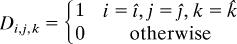
3. For r = 1 … R, Resp_r ← p_r^α/ Σ_np_n^α

4. For r = 1 … R, and for all i, j, k

   

   

5. r̂ ← arg max{Resp_r}; mix _r̂ ← mix _r̂ + η

6. For r = 1 … R, mix _r = mix _r/ Σ_n mix_n.

Each run had 40,000 trials with learning rate η = 0.001. G is the plasticity kernel, defined to be G(i, j, k) = exp(−[i² + j² + k²]); α is a “sharpening” parameter, set to 1.15 (α > 1 assigns greater responsibility to the winning unit). For efficiency, a category was eliminated once its mix_r fell to <0.001, and the update of the conditional probabilities was restricted to input units for which plasticity kernel G(·) > 0.01.

Abbreviations

EM

Expectation–Maximization

F1

first formant

F2

second formant

OME

Online Mixture Estimation

TOME

Topographic OME.

References

- 1.Werker JF, Gilbert JHV, Humphrey GK, Tees RC. Child Dev. 1981;52:349–355. [PubMed] [Google Scholar]
- 2.Kuhl PK, Stevens E, Hayashi A, Deguchi T, Kiritani S, Iverson P. Dev Sci. 2006;9:13–21. doi: 10.1111/j.1467-7687.2006.00468.x. [DOI] [PubMed] [Google Scholar]
- 3.Bosch L, Sebastián-Gallés N. Lang Speech. 2003;46:217–243. doi: 10.1177/00238309030460020801. [DOI] [PubMed] [Google Scholar]
- 4.Best CT, McRoberts GW, Sithole NM. J Exp Psychol Human. 1988;14:345–360. doi: 10.1037//0096-1523.14.3.345. [DOI] [PubMed] [Google Scholar]
- 5.Werker JF, Tees RC. Infant Behav Dev. 1984;7:49–63. [Google Scholar]
- 6.Burns TC, Yoshida KA, Hill K, Werker JF. Appl Psycholinguist. 2007;28:455–474. [Google Scholar]
- 7.Aslin RN, Pisoni DB. In: Perception. Yeni-Komshian GH, Kavanagh JF, Ferguson CA, editors. Vol 2. New York: Academic; 1980. pp. 67–96. Child Phonology. [Google Scholar]
- 8.Guenther FH, Gjaja MN. J Acoust Soc Am. 1996;100:1111–1121. doi: 10.1121/1.416296. [DOI] [PubMed] [Google Scholar]
- 9.Vallabha GK, McClelland JL. Cognit Affect Behav Neurosci. 2007;7:53–73. doi: 10.3758/cabn.7.1.53. [DOI] [PubMed] [Google Scholar]
- 10.Kuhl PK, Williams KA, Lacerda F, Stevens KN, Lindblom B. Science. 1992;255:606–608. doi: 10.1126/science.1736364. [DOI] [PubMed] [Google Scholar]
- 11.Polka L, Werker JF. J Exp Psychol Human. 1994;20:421–435. doi: 10.1037//0096-1523.20.2.421. [DOI] [PubMed] [Google Scholar]
- 12.Maye J, Werker JF, Gerken L. Cognition. 2002;82:B101–B111. doi: 10.1016/s0010-0277(01)00157-3. [DOI] [PubMed] [Google Scholar]
- 13.Maye J, Weiss D, Aslin RN. Dev Sci. doi: 10.1111/j.1467-7687.2007.00653.x. in press. [DOI] [PubMed] [Google Scholar]
- 14.Bernstein-Ratner N. J Child Lang. 1984;11:557–578. [PubMed] [Google Scholar]
- 15.Kuhl PK, Andruski JE, Chistovich IA, Chistovich LA, Kozhevnikova EV, Ryskina VL, Stolyarova EI, Sundberg U, Lacerda F. Science. 1997;277:684–686. doi: 10.1126/science.277.5326.684. [DOI] [PubMed] [Google Scholar]
- 16.Fernald A, Taeschner T, Dunn J, Papousek M, Boysson-Bardies B, Fukui I. J Child Lang. 1989;16:477–501. doi: 10.1017/s0305000900010679. [DOI] [PubMed] [Google Scholar]
- 17.Werker JF, Pons F, Dietrich C, Kajikawa S, Fais L, Amano S. Cognition. 2007;103:147–162. doi: 10.1016/j.cognition.2006.03.006. [DOI] [PubMed] [Google Scholar]
- 18.Westermann G, Miranda ER. Brain Lang. 2004;89:393–400. doi: 10.1016/S0093-934X(03)00345-6. [DOI] [PubMed] [Google Scholar]
- 19.Guenther FH, Nieto-Castanon A, Ghosh SS, Tourville JA. J Speech Lang Hear R. 2004;47:46–57. doi: 10.1044/1092-4388(2004/005). [DOI] [PubMed] [Google Scholar]
- 20.Gauthier B, Shi R, Xu Y. Cognition. 2007;103:80–106. doi: 10.1016/j.cognition.2006.03.002. [DOI] [PubMed] [Google Scholar]
- 21.Duda RO, Hart PE, Stork DG. Pattern Classification. New York: Wiley; 2000. [Google Scholar]
- 22.de Boer B, Kuhl PK. Acoust Res Lett Onl. 2003;4:129–134. [Google Scholar]
- 23.Coen MH. Proceedings of the 20th National Conference on Artificial Intelligence (AAAI'06); Menlo Park, CA: AAAI Press; 2006. [Google Scholar]
- 24.McMurray B, Aslin RN, Toscano J. Dev Sci. doi: 10.1111/j.1467-7687.2009.00822.x. in press. [DOI] [PMC free article] [PubMed] [Google Scholar]
- 25.Grossberg S. J Phonetics. 2003;31:423–445. [Google Scholar]
- 26.Rumelhart DE, Zipser D. Cognit Sci. 1985;9:75–112. [Google Scholar]
- 27.Kohonen T. Neural Networks. 1993;6:895–905. [Google Scholar]
- 28.Rosenthal O, Fusi S, Hochstein S. Proc Natl Acad Sci USA. 2001;98:4265–4270. doi: 10.1073/pnas.071525998. [DOI] [PMC free article] [PubMed] [Google Scholar]
- 29.Pijpers M, Alder MD, Togneri R. First Australian and New Zealand Conference on Intelligent Information Systems, Perth, Australia. Menlo Park, CA: IEEE Press; 1993. [Google Scholar]
- 30.Vallabha GK, Tuller B. J Acoust Soc Am. 2004;116:1184–1197. doi: 10.1121/1.1764832. [DOI] [PubMed] [Google Scholar]
- 31.Rosseel Y. J Math Psychol. 2002;46:178–210. [Google Scholar]
- 32.Lively SE, Logan JS, Pisoni DB. J Acoust Soc Am. 1993;94:1242–1255. doi: 10.1121/1.408177. [DOI] [PMC free article] [PubMed] [Google Scholar]
- 33.Silverman BW. Density Estimation for Statistics and Data Analysis. Boca Raton, FL: Chapman & Hall/CRC; 1986. [Google Scholar]
- 34.Oja E. J Math Biol. 1982;15:267–273. doi: 10.1007/BF00275687. [DOI] [PubMed] [Google Scholar]
- 35.O'Reilly RC, Munakata Y. Computational Explorations in Cognitive Neuroscience. Cambridge, MA: MIT Press; 2000. [Google Scholar]
- 36.Gold JI, Shadlen MN. Trends Cognit Sci. 2001;5:10–16. doi: 10.1016/s1364-6613(00)01567-9. [DOI] [PubMed] [Google Scholar]
- 37.Poggio T. Cold Spring Harb Symp. 1990;55:899–910. doi: 10.1101/sqb.1990.055.01.084. [DOI] [PubMed] [Google Scholar]
- 38.Petrov A, Dosher BA, Liu Z-L. Psychol Rev. 2005;112:715–743. doi: 10.1037/0033-295X.112.4.715. [DOI] [PubMed] [Google Scholar]
- 39.Kersten D, Yuille A. Curr Opin Neurobiol. 2003;13:1–9. doi: 10.1016/s0959-4388(03)00042-4. [DOI] [PubMed] [Google Scholar]
- 40.Neal RM, Hinton GE. In: Learning in Graphical Models. Jordan MI, editor. Cambridge, MA: MIT Press; 1999. pp. 355–368. [Google Scholar]
- 41.Roberts SJ, Husmeier D, Rezek I, Penny W. IEEE T Pattern Anal. 1998;20:1133–1142. [Google Scholar]
- 42.Marin J-M, Mengersen K, Robert CP. In: Handbook of Statistics. Dey D, Rao CR, editors. Vol 25. London: Elsevier Sciences; 2005. pp. 459–507. [Google Scholar]
- 43.Johnson K. In: Talker Variability in Speech Processing. Johnson K, Mullennix JW, editors. San Diego: Academic; 1997. pp. 145–165. [Google Scholar]
- 44.Andruski JE, Nearey TM. J Acoust Soc Am. 1992;91:390–410. doi: 10.1121/1.402781. [DOI] [PubMed] [Google Scholar]
- 45.Zahorian SA, Jagharghi AJ. J Acoust Soc Am. 1993;94:1966–1982. doi: 10.1121/1.407520. [DOI] [PubMed] [Google Scholar]
- 46.Kawamoto A, Anderson J. Acta Psychol. 1985;59:35–65. doi: 10.1016/0001-6918(85)90041-1. [DOI] [PubMed] [Google Scholar]
- 47.Schouten MEH, van Hessen A. J Acoust Soc Am. 1998;104:2980–2990. doi: 10.1121/1.423880. [DOI] [PubMed] [Google Scholar]
- 48.Maddox WT, Bogdanov SV. Percept Psychophys. 2000;62:984–997. doi: 10.3758/bf03212083. [DOI] [PubMed] [Google Scholar]
- 49.McClelland JL. In: Leading Themes. Bertelson P, Eelen P, d'Ydewalle G, editors. Vol 1. East Sussex, UK: Erlbaum; 1994. pp. 57–88. International Perspectives on Psychological Science. [Google Scholar]
- 50.Plaut DC, McClelland JL, Seidenberg MS, Patterson K. Psychol Rev. 1996;103:56–115. doi: 10.1037/0033-295x.103.1.56. [DOI] [PubMed] [Google Scholar]
- 51.Hoffbeck JP, Landgrebe DA. IEEE T Pattern Anal. 1996;18:763–767. [Google Scholar]
Associated Data
This section collects any data citations, data availability statements, or supplementary materials included in this article.