Abstract
The conformational transition states of a β-hairpin peptide in explicit water were identified from the free energy landscapes obtained from the multicanonical ensemble, using an enhanced conformational sampling calculation. The β-hairpin conformations were significant at 300 K in the landscape, and the typical nuclear Overhauser effect signals were reproduced, consistent with the previously reported experiment. In contrast, the disordered conformations were predominant at higher temperatures. Among the stable conformations at 300 K, there were several free energy barriers, which were not visible in the landscapes formed with the conventional parameters. We identified the transition states around the saddle points along the putative folding and unfolding paths between the β-hairpin and the disordered conformations in the landscape. The characteristic features of these transition states are the predominant hydrophobic contacts and the several hydrogen bonds among the side-chains, as well as some of the backbone hydrogen bonds. The unfolding simulations at high temperatures, 400 K and 500 K, and their principal component analyses also provided estimates for the transition state conformations, which agreed well with those at 400 K and 500 K deduced from the current free energy landscapes at 400 K and 500 K, respectively. However, the transition states at high temperatures were much more widely distributed on the landscape than those at 300 K, and their conformations were different.
Keywords: β-hairpin peptide, energy landscape, multicanonical molecular dynamics, peptide folding, principal component analysis
The transition states between the ordered and disordered conformations of peptides and proteins govern their folding and unfolding reactions. These transition states significantly differ from those of other chemical reactions, which are generally accompanied by the introduction, removal, or modification of a covalent bond in a molecule. Instead, they are referred to as the conformational transition states with a high free energy between the ordered and disordered conformations, and many studies have sought to clarify their energetics and conformations (Brooks 1998; Baldwin and Rose 1999; Arai and Kuwajima 2000). The thermodynamic behaviors of the transition states have been revealed by kinetic experiments combined with thorough amino acid mutations to deduce the φ values for the individual residues, from which the structural images for the transition states can be investigated (Fersht 1995). However, since single-molecule observations for the transition state have not yet been made, all of the above views were for the averaged structures in the ensemble at the transition states. Thus, a theoretical support is required to obtain more precise information for the energies and the structures of the conformational transition state.
Li and Daggett (1994) first explored the conformational transition states of chymotrypsin inhibitor 2 from the unfolding molecular dynamics (MD) simulation at high temperature (498 K) at an atomic resolution. The transition states from the unfolding MD simulations at high temperature were estimated by a conformational cluster analysis using the principal component analysis (PCA). In many cases, their results were consistent with the experiments, particularly for the φ values, but there was no energetic or conformational evidence to provide a correct picture for the transition states near room temperature in their computations. Since their pioneering studies, the landscape theorem for protein folding has become popular, and the transition states have been investigated from the free energy landscapes by exhaustive or enhanced conformational searches for lattice models or coarse-grained models (Onuchic et al. 1996; Muñoz et al. 1998; Galzitskaya and Finkelstein 1999; Alm and Baker 1999; Chikenji and Kikuchi 2000), and for more precise atomic models with implicit water solvent (Dinner et al. 1999; Zagrovic et al. 2001). The transition states examined by these studies were certainly more reliable with the calculated free energy values than before, because of the technical development of enhanced conformational sampling (Hansmann and Okamoto 1993). However, the models for peptides and proteins were more or less simplified. In particular, the contributions of hydrophobic interactions were often assumed beforehand. Moreover, the free energy landscapes were drawn with arbitrary axes, such as the radius of gyration rG, the solvent accessible surface area (ASA) of the solute molecules, and the native contacts. Although these parameters can well discriminate the native structure from the unfolded one, it is not clear whether such projections to a couple of conventional arbitrary axes would yield a correct understanding of the conformational transition state distribution.
We recently developed a new simulation method, multicanonical molecular dynamics (McMD), which provides an enhanced conformational search for a precise atomic model of peptides and proteins (Nakajima et al. 1997, 2000; Shirai et al. 1998; Kim et al. 1999). The replica-exchange method also provides a similar enhanced diversity search of peptides (Sugita and Okamoto 1999; García and Sanbonmatsu 2001). Using these generalized ensemble methods, the free energy landscapes of short peptides in explicit water have now been obtained, after determining the appropriate principal axes with the PCA method (García and Sanbonmatsu 2001; Higo et al. 2001a,b).
Among short peptides, a β-hairpin is an interesting target for studies of conformational transition states, because it is formed mainly by long-range interactions along the peptide chain. The long-range interactions are very different from the interactions needed to form an α-helix, and are believed to be more similar to those of large proteins. Stable β-hairpins in aqueous solvent have been proposed (Ramírez-Alvarado et al. 1996; Honda et al. 2000), and several simulations, including our previous study (Higo et al. 2001a) also predicted their existence near room temperature from the free energy landscapes. However, the landscapes obtained by the PCA method generally have accuracy problems. Here we propose a new method to provide a precise energy landscape, after an enhanced conformational search with the McMD method. With this method, the conformational transition states of a β-hairpin were identified and characterized in detail along the transition pathways between the ordered and disordered conformations.
Results
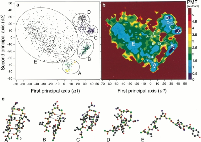
The sequence of the peptide was [Ace1-Ile2-Thr3-Val4-Asn5-Gly6-Lys7-Thr8-Tyr9-Nme10]. This sequence is derived from a de novo designed β-hairpin peptide (Ramírez-Alvarado et al. 1996), which has the additional residues Arg-Gly- and -Gly-Arg at the N- and C-termini, respectively, to increase the solubility. Here, they were deleted to reduce the system size. The amino acid residue Lys7 was treated as being fully charged. Figure 1a ▶ shows the conformational distribution of the canonical ensemble at 300 K, Q(300 K), plotted against the principal axes a1 and a2, corresponding to the largest and the second largest eigen vectors given by the quasiharmonic analysis (Teeter and Case 1990; Kitao et al. 1991; Amadei et al. 1993; Higo and Umeyama 1997). The conformational distribution in Figure 1a ▶ is essentially similar to that obtained in our previous study (Higo et al. 2001a), where the axes were determined by PCA for the randomly selected conformations in Q(300 K). Thus, our current quasiharmonic method is as effective as the usual PCA in providing the landscapes.
Fig. 1.
(a) Distribution of 2064 conformations in Q(300 K) obtained from McMD and quasiharmonic analysis. Five clusters, A–E, with circles are shown in the figure. Black dots are for the 0HB conformation, blue for 1HB, green for 2HB, yellow for 3HB, and red for 4HB. The λi/Σλi was 35% (i = 1), 15% (i = 2), 8% (i = 3), 5% (i = 4), 5% (i = 5), 4% (i = 6), and so on. Here, λi was the eigen value assigned to the ith axis. The eigen values were arranged in descending order. (b) Free energy landscape at 300 K obtained from McMD and quasiharmonic analysis. It was drawn with the bin size 3.0 × 3.0. The contour value in kcal/mol is shown on the right side of the figure. Each white dot is the local minimum for the corresponding stable conformation from clusters A to D. Four conformational transition states, A ― E, B ― E, D ― E, and C ― D, with white dotted circles, are shown in the figure. (c) Typical structures in clusters A–E with the hydrogen bonds (broken lines). Green atoms are for Cα, black for other C, red for O, and blue for N. Backbones are shown in yellow. Residue numbers are given near the corresponding Cα atoms. The pictures were drawn by MOLSCRIPT (Kraulis 1991) and Raster3D (Merritt and Murphy 1994).
In Figure 1a ▶, five clusters, A–E, were found. We plotted the conformational distribution against other principal axes, that is, a1 and a3, etc., but no more remarkable clusters than those shown in the figure were found. Therefore, we characterized the conformations using the five clusters. The complete β-hairpin contains four characteristic hydrogen bonds between the backbone atoms: 2HN-9O, 2O-9HN, 4HN-7O, and 4O-7HN. Here, iHN and iO were the amide hydrogen and the carbonyl oxygen of the ith residue, respectively. A conformation with k of the above four hydrogen bonds is denoted as the kHB conformation below. The hydrogen bond, 4O-7HN, participates in the β-turn formation. The numbers of kHB conformations in Q(300 K) were 1384 (67.1%, k = 0), 453 (21.9%, k = 1), 203 (9.8%, k = 2), 23 (1.1%, k = 3), and 1 (0.05%, k = 4), respectively.
In cluster A, the hydrogen bonds 2HN-9O, 2O-9HN, and 4HN-7O were predominantly observed, with a rare hydrogen bond (4O-7HN) for the β-turn. A significant hydrophobic core is formed by the side chain contacts between Ile2 and Val4, between Thr3 and Thr8, and between the side-chain stems of Lys7 and Tyr9. Remarkably, in cluster B, the β-turn and the 4HN-7O hydrogen bond were observed with the same hydrophobic core. In cluster C, only a hydrogen bond forming the β-turn was found. In cluster D, other backbone hydrogen bonds, 6HN-9O, 4O-8HN, or 4O-9HN, were observed. In particular, the hydrogen bond, 4O-8HN, constructs an α-helical turn. Cluster E corresponds to the disordered random conformation with the 0HB conformation, and forms no secondary structure. Typical conformations of these clusters are shown in Figure 1c ▶.
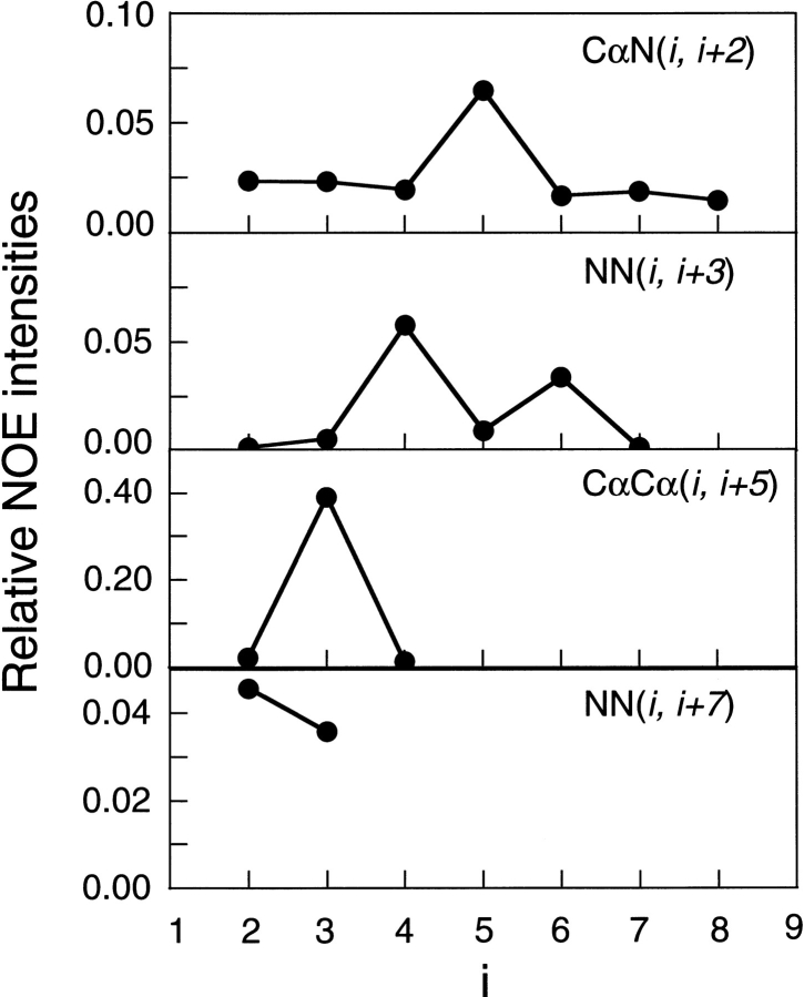
In Q(300 K), 33% conformations assumed the β-hairpins for k ≥1. To confirm the reliability of the current conformational ensemble, the nuclear Overhauser effect (NOE) intensities between the peptide backbone atoms in Q(300 K) were examined and compared with the experimental results (Ramírez-Alvarado et al. 1996). Figure 2 ▶ shows the NOE intensities at CαN(i, i+2), NN(i, i+3), CαCα(i, i+5), and NN(i, i+7) from Q(300 K) with the whole 2064 structures indicated in Figure 1a ▶. The intense NOE signals were found at CαN(5, 7), NN(4, 7), CαCα(3, 8), and NN(2, 9). They were consistent with the experimental data (Ramírez-Alvarado et al. 1996). However, the intense NOE signals at NN(6, 9) and NN(3, 10), INN(6, 9) and INN(3, 10), respectively, found in our simulation, were not observed in the experiment. To examine the conformations which contributed to INN(6, 9) and INN(3, 10), we picked up 38 and 40 conformations that were satisfied with the NOE signals INN(6, 9), INN(3, 10) > 0.001, respectively. The former conformations with the NN(6, 9) signal mainly contained two hydrogen bonds, 4O-7HN and 4HN-8O. The latter one, with NN(3, 10), had two hydrogen bonds, 4O-9HN and 6HN-9O. Thus, the intense INN(6, 9) and INN(3, 10) signals were derived from cluster D in Figure 1a and b ▶.
Fig. 2.
NOE intensities obtained from Q(300 K) at CαN(i, i+2), NN(i, i+3), CαCα (i, i+5), and NN(i, i+7). The signals between the ith Cα hydrogen and the i+jth amide hydrogen, between the ith amide hydrogen and the i+jth amide hydrogen, and between the ith Cα hydrogen and the i+jth Cα hydrogen are shown by CαN(i, i+j), NN(i, i+j), and CαCα (i, i+j), respectively.
The free energy landscape at a given temperature T was obtained from the potential of mean force (PMF) of Q(T) for a1 and a2. The probability distribution ρ(a1, a2, T) gives the PMF, F(a1, a2, T) = −RT ln ρ(a1, a2, T), where R is the gas constant. The PMF was shifted so it would be zero at its global minimum. In Figure 1b ▶, the free energy landscape at 300 K is mapped on the same space using the axes in Figure 1a ▶. The region for the disordered conformations (cluster E) exhibited a rugged surface. The local PMF minima in clusters A–D are listed in Table 1. Each PMF value does not directly coincide with the degree of the stability. The boundary region between clusters A and B, where the complete β-hairpin conformations were occasionally located, was not very stable due to their small entropy and rare probability. The PMF minimum in cluster E was not determined because of the rugged landscape. Narrow paths were found as the conformational transitions between A ― B, B ― C, A ― E, B ― E, C ― D, C ― E, and D ― E. The energy barrier in the transitions between clusters and the location of the saddle points via the corresponding minimum energy path are listed in Table 1. As shown in Table 2, the energy barrier of ΔFA→E was approximately constant, whereas that of ΔFB→E decreased with increasing temperature in the region from 300 to 360 K. The free energy landscapes at the individual temperatures are shown in the Supplementary material.
Table 1.
Potential of mean force ( F) of the local minimum in each cluster from A to E, and energy barrier (ΔFX → Y) in the transitions from the clusters X to Y at 300 K
| Clusters (X) | A | B | C | D |
| F (kcal/mol) at local minimum | 0.8 (6.5, −43.5)a | 0.1 (33.5, −16.5)a | 0.0 (39.5, 10.5)a | 0.3 (30.5, 28.5)a |
| ΔFX → A (kcal/mol) | — | 2.5 (18.5, −37.5)b | c—c | —c |
| ΔFX → B (kcal/mol) | 1.8 (18.5, −37.5)b | — | 2.0 (27.5, −4.5)b | —c |
| ΔFX → C (kcal/mol) | —c | 1.9 (27.5, −4.5)b | — | 1.5 (33.5, 16.5)b |
| ΔFX → D (kcal/mol) | —c | —c | 1.8 (33.5, 16.5)b | —c |
| ΔFX → E (kcal/mol) | 0.5 (0.5, −37.5)b | 2.0 (21.5, −7.5)b | 2.1, 2.2d | 1.8 (12.5, 7.5)b |
a, b The numbers in the parentheses (a1, a2) indicate the location of the local minima and the transition states, respectively, in the landscapes in Fig. 1a and b ▶.
c There is no direct path for the transition.
d The transition C ― E should go through the same path as either B ― E or D ― E.
Table 2.
Free energy barrier at the transitions from clusters A to E, and B to E at 300–360 K
| Temperature (K) | ΔFA → E (kcal/mol) | ΔFB → E (kcal/mol) |
| 300 | 0.5 (6.5, −43.5)a, (0.5, −37.5)b | 2.0 (33.5, −16.5)c, (21.5, −7.5)d |
| 320 | 1.0 (3.5, −49.5)a, (0.5, −40.5)b | 2.1 (30.5, −16.5)c, (15.5, −1.5)d |
| 340 | 0.7 (6.5, −43.5)a, (3.5, −34.5)b | 1.8 (27.5, −22.5)c, (21.5, −16.5)d |
| 360 | 0.9 (9.5, −40.5)a, (−5.5, −34.5)b | 1.6 (33.5, −16.5)c, (24.5, −7.5)d |
a–d The numbers in the parentheses (a1, a2) indicate the location of the local minima at cluster A, the transition states at A ― E, the local minima at cluster B, and the transition states at B ― E, respectively. The free energy landscapes at the individual temperatures are shown in the supplemental material.
The disordered conformation was more stable at 400 K and 500 K, as shown in Figure 3a and b ▶, respectively, and at higher temperatures (data not shown). A wide basin with low PMF values was located in the disordered conformation region, and the high free energy barrier around (a1, a2) = (15, −25), found at 300 K, disappeared. Thus, the transition between the ordered and disordered conformations should occur via multiple paths at 400 K and 500 K and at higher temperatures.
Fig. 3.
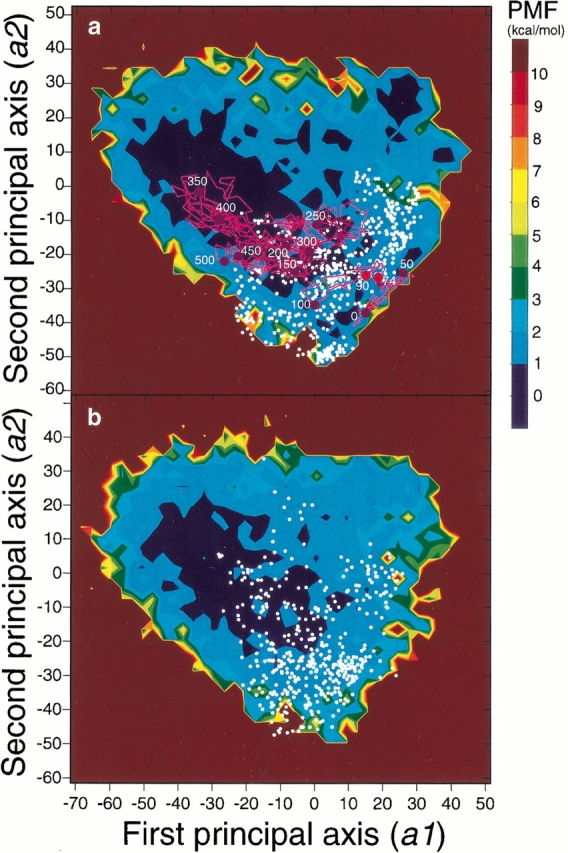
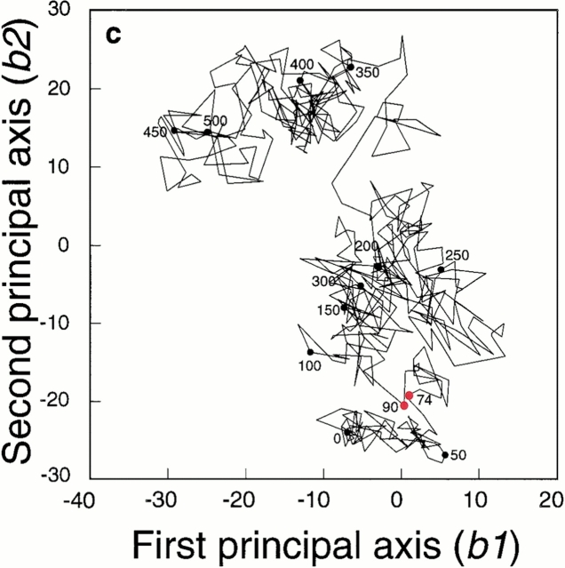
(a) Free energy landscape at 400 K obtained from McMD and quasiharmonic analysis. The contour value in kcal/mol is shown on the right side of the figure. The unfolding trajectory at 400 K was superimposed on the landscape with pink lines and circles. The white dots correspond to the locations of the transition states estimated from 25 different unfolding simulations at 400 K. (b) Free energy landscape at 500 K obtained from McMD and quasiharmonic analysis. The contour value is the same as in Fig. 3a ▶. The white dots correspond to the locations of the transition states estimated from 25 different unfolding simulations at 500 K. (c) Unfolding trajectory at 400 K analyzed with the PCA method. The simulation time is shown in the figure in ps. The red solid circles are the initial (74 ps) and the final (90 ps) points for the transition state.
Unfolding MD simulations at 400 K and 500 K were carried out starting from 25 different β-hairpin conformations. Each unfolding trajectory was different and followed an individual pathway. In Figure 3c ▶, the PCA projection for one of the unfolding trajectories at 400 K is shown to estimate the transition state. The conformations from 74 to 90 ps formed the significant cluster in the first and the second principal axes (b1 and b2, respectively). We assigned this cluster as the unfolding transition state, following the method of Li and Daggett (1994). In this cluster, the native hydrogen bonds were lost, and only the hydrophobic interactions were kept. This unfolding trajectory was also mapped on the free energy landscape at 400 K, shown in Figure 3a ▶. The cluster from 74 to 90 ps has PMF values only above 1 kcal/mol, and it is located near (a1, a2) = (15, −25), where a transition would be forbidden at 300 K, since the free energy barrier is more than 5 kcal/mol.
In addition, the transition states thus estimated from 25 unfolding simulations starting from different initial ordered conformations are superimposed on the free energy landscape at 400 K and 500 K (small white points in Fig. 3a and b ▶), respectively. Although the transition states at both temperatures are widely distributed throughout the ordered and disordered conformation regions, most of the conformations are found between them. Moreover, the transition states at 500 K were more widely distributed than those at 400 K. Thus, the transition state information provided by the unfolding simulations is similar to that from the landscape analysis at the corresponding temperature. However, these transition states were clearly different from those at 300 K, as shown in Figure 1b ▶. The numbers of conformations with typical β-hairpin hydrogen bonds were 10/28 structures at 300 K and 13/130 structures at 400 K. The average numbers of the native and nonnative contacts between side-chain atoms in the transition state at 400 K were 4.32 and 4.82, respectively, which were different from those at 300 K (5.54 for native contact, 3.68 for nonnative contact). The detailed properties of the transition at 300 K are given in the Discussion.
Figure 4 ▶ shows (1) the corresponding distance changes between four hydrogen bond pairs, (2) the ASA, and (3) the native and nonnative contacts, during the unfolding trajectory at 400 K. The most terminal hydrogen bond, 2HN-9O, between the strands was first broken at 46 ps, and after 74 ps, none of the four β-hairpin hydrogen bonds was formed. As shown in Figure 4b ▶, the ASA was between ∼1100 and 1200 Å2 from 74 to 90 ps. Once the β-hairpin conformation was completely broken, the ASA was over ∼1300 Å2. The ASA contributed by only the hydrophobic portions of the side chains (hydrophobic ASA) also displayed a similar change during the unfolding process, as shown by the dotted line in Figure 4b ▶. In the following discussion, only this hydrophobic ASA is discussed. In Figure 4c ▶, the numbers of native and nonnative contacts between the side-chain atoms are plotted along the trajectory. About half of the native contacts, which are defined as the contacts in the initial β-hairpin structure of the unfolding, were maintained from 74 to 90 ps. In particular, the native contact between Thr3 and Thr8, which preserves the strand conformation via the hydrophobic interaction between both side-chain methyl groups, was maintained.
Fig. 4.
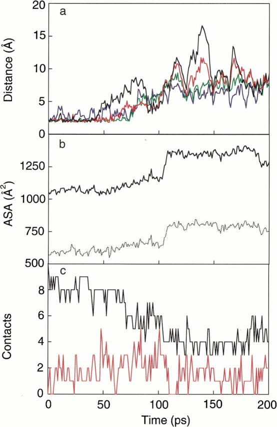
(a) Hydrogen bond pair distances (black for the distance between 2HN and 9O, red for 2O and 9HN, green for 4HN and 7O, and blue for 4O and 7HN), (b) total (solid line) and hydrophobic ASA (dotted line), and (c) native (black line) and nonnative (red line) contact numbers, along a typical unfolding trajectory at 400 K starting from a complete β-hairpin conformation.
Discussion
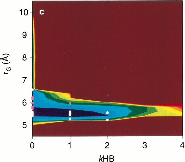
Thus far, it has been difficult to draw realistic free energy landscapes of a β-hairpin peptide with explicit water, because of the limitations of the conformational sampling and the precision of the models. In addition, the axes of the landscapes were often not objective, but were selected arbitrarily, using the conventional parameters. For example, the radius of gyration rG, the ASA, and the root mean square deviation (r.m.s.d.) from the native structure have often been used to display the landscapes (Sheinerman and Brooks III 1998; Alm and Baker 1999; Dinner et al. 1999; Zagrovic et al. 2001). When these axes are used to display the landscape for the current ensemble at 300 K, Figure 5a, b, and c ▶ are obtained. In contrast to Figure 1b ▶, with its rugged landscape given by the (3n-6)-dimensional analysis, these landscapes are very smooth and funnel-like. The transition state conformations found from Figure 1b ▶ are also represented in Figure 5a, b, and c ▶ by white (A ― E) and pink (B ― E) dots. These projections to arbitrary axes are not appropriate to identify the transition states or to analyze the folding and unfolding mechanism in the present study.
Fig. 5.
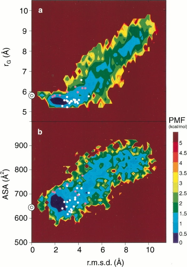
Free energy landscapes at 300 K drawn by the conventional arbitrary axes. (a) The radius of gyration rG and the r.m.s.d. from the ordered conformation, (b) the hydrophobic ASA and the r.m.s.d., and (c) rG and the numbers of kHB were used. The contour value in kcal/mol is shown on the right side of the figure. The double circles on the axis at r.m.s.d. = 0 are the positions for the ordered conformation. White and pink dots are the transition state conformations at A ― E and at B ― E in Fig. 1b ▶, respectively.
The PCA method applied in our previous procedure (Higo et al. 2001a,b) and by García and Sanbonmatsu (2001) provides objective axes, which are much better than the aforementioned conventional parameters. However, the PCA method requires all of the conformations to diagonalis the distance matrix between conformations, and so the precision of the probability distribution is limited, due to the technical reason of computer memory space. Moreover, it is difficult to map conformations other than those used in PCA. Our current quasiharmonic analysis has an advantage over PCA, because the precise probability distribution can be provided by using the multitude of conformations in the ensemble, and conformations such as those during the unfolding trajectory are projected on the same landscape.
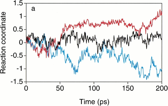
In addition to the unfolding simulation analysis, another method to identify the conformational transition state was proposed as the P½ analysis (Pande and Rokhsar 1999). Since the transition state is located at the saddle point, a short MD simulation starting from a candidate conformation should quickly produce or deform the ordered conformation. When starting from a correct transition state conformation, the probability to produce the ordered conformation should be ½. Here, as indicated in Figure 5c ▶, the number of kHB is not considered to be a good measure as the reaction coordinate. We therefore observed the direction of the conformational change, by defining another reaction coordinate as the projection to the line, connecting the starting point and the local minimum A or B in the landscape at 300 K (see Materials and Methods). For the trajectories just around the starting points, this reaction coordinate equals 0 at the starting point. It equals 1 at the local minimum A or B, and it is negative when the peptide deforms.
Typical trajectories are shown in Figure 6a ▶, and it was found that the directions of the conformational change were all determined around 100 ps. Thus, the distributions of the reaction coordinates averaged during 50 to 150 ps are shown for the path A ― E in Figure 6b ▶, and for the path B ― E in Figure 6c ▶. As shown in Figure 6b ▶, about half of the collection of 20 simulations starting from the point AE1 were located in the ordered direction, and the other half were in the disordered direction. In contrast, the points of AE2 and AE3 were slightly near the ordered conformation A. As shown in Figure 6c ▶, the point BE3 was close to the correct transition state with nearly the ½ probability, and the points BE1 and BE2 were slightly near the deformed conformation E. Thus, the transition state conformations identified from the current free energy landscape are consistent with those given by the P½ analysis.
Fig. 6.
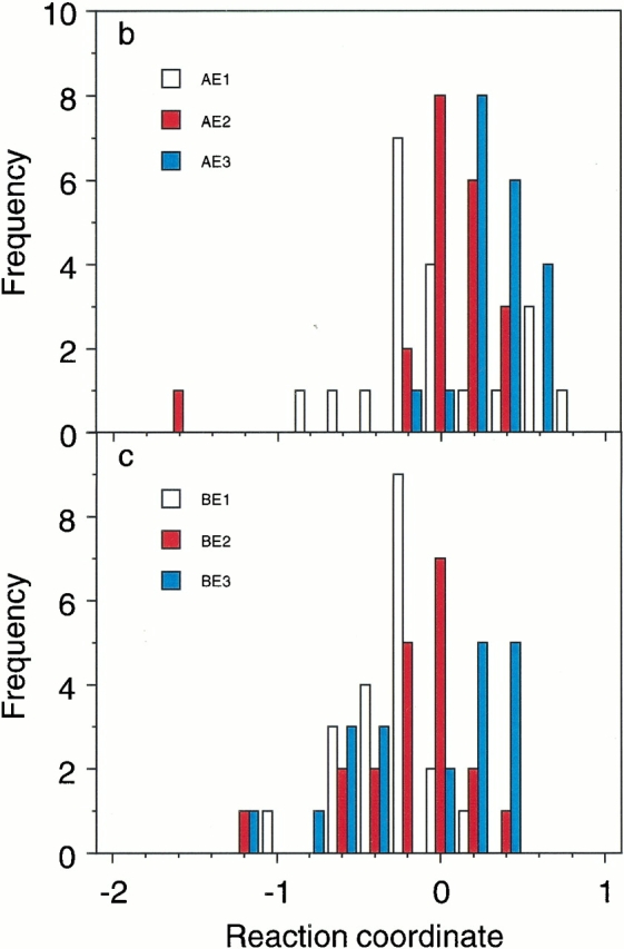
Results of the P½ analysis. (a) Three trajectories of the short canonical MD simulations at 300 K starting from the candidate transition state named AE1 at (a1, a2) = (−3.0, −33.7) in the free energy landscape shown in Fig. 1b ▶. The longitudinal axis indicates the reaction coordinates defined in the text (Materials and Methods). The averages of the reaction coordinates during 50 to 150 ps were 0.68 (red), 0.10 (black), and −0.53 (blue). The trajectories after 10 ps heating were plotted. (b) Distributions of the averages of the reaction coordinates during 50 to 150 ps for the three simulations starting from the candidate transition state conformations at A ― E: AE1, AE2 at (a1, a2) = (4.5, −37.6), and AE3 at (a1, a2) = (0.1, −35.6). (c) Distributions of the averages of the reaction coordinates during 50 to 150 ps for the three simulations starting from the candidate transition state conformations at B ― E: BE1 at (a1, a2) = (15.3, −9.4), BE2 at (a1, a2) = (20.9, −5.9), and BE3 at (a1, a2) = (23.4, −5.7).
Consequently, within the precise free energy landscape at 300 K (Fig. 1b ▶), two folding paths were clearly observed. The path A ― E corresponds to the folding mechanism of a β-hairpin, in which the N- and C-termini of the peptide first approach each other to form a loop, and then the β-turn is constructed at the final stage (Pande and Rokhsar 1999). In contrast, along the path B ― E, the β-turn is formed first, and then the hydrogen bond ladder is gradually made (Muñoz et al. 1997). These two mechanisms have been controversial, but it is now evident from our free energy landscape that both mechanisms are possible, following the path A ― E or the path B ― E. This conclusion is similar to that suggested by Dinner et al. (1999). However, the energy barrier of ΔFA → E was lower than that of ΔFB→E around 300 K, and so the folding path A ― E could be more favorable than that of B ― E. Interestingly, as indicated in Table 2, the energy barrier of ΔFA→E became close to that of ΔFB→E at higher temperature.
As shown in Figure 7a ▶, the ordered conformational ensemble exhibited a small hydrophobic ASA, while the disordered ensemble had a large hydrophobic ASA. At the transition states, the slight increase of the ASA distribution from the ordered conformations is due to the partial destruction of the ordered β-hairpin structure, which caused several atoms to become newly exposed to the solvent. The conformations with typical β-hairpin hydrogen bonds composed 35.5% of the transition states (Fig. 7b ▶). In addition, among the 28 transition state conformations picked from Q(300 K), we observed (1) 21% of the native hydrophobic contacts, (2) two conformations with a nonnative hydrophobic contact between Val4 and Lys7 to pack the strands, (3) 10 conformations with typical β-hairpin backbone hydrogen bonds, and (4) 10 conformations with hydrogen bonds between the side-chain atoms (Thr3 and Thr8, or Lys7 and Tyr9). These results indicate that the hydrophobic collapse and some of the hydrogen bonds between the backbone atoms and between the side chains are essential features of the transition states.
Fig. 7.
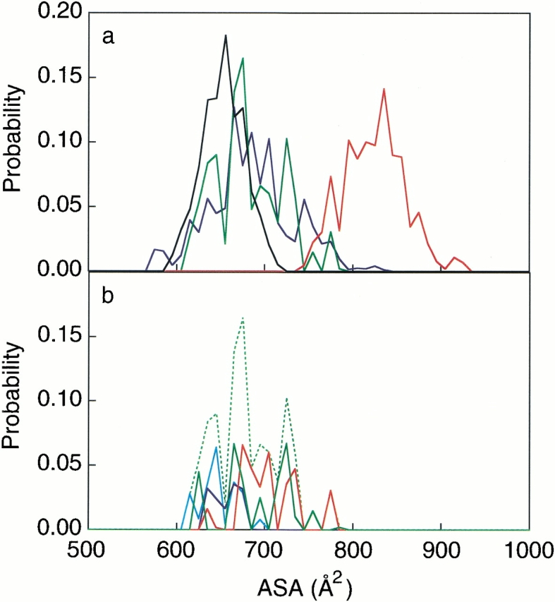
(a) Probability distribution of the hydrophobic ASA values for the ordered conformation (black), the disordered conformation (red), the transition state ensemble at 300 K (green), and the transition state ensemble at 400 K (blue), picked from the landscapes. (b) Probability distribution of the hydrophobic ASA for the transition states at 300 K. The blue line is contributed from 2HB, the sky blue line is from 1HB, the green line is from a conformation with other hydrogen bonds, and the red line is from a conformation without any intramolecular hydrogen bonds. The broken green line is the total summation.
In the transition state conformations at A ― E and at B ― E, the number of water molecules forming hydrogen bonds with the atoms participating in kHB was 6.1/structure. In contrast, it was 4.3/structure in the ordered conformations at clusters A and B, and 7.7/structure in the disordered conformations at cluster E. Thus, water molecules penetrating into the strands also contributed toward stabilizing the transition states.
In Figure 7a ▶, the ASA distribution of the transition states is broader than that of the ordered conformations, and actually, it is as broad as that of the disordered conformations. This suggests that the transition states should be stabilized from the large conformational entropy by a combination of different hydrophobic contacts and various transition paths, as once suggested for a simplified model protein (Galzitskaya and Finkelstein 1999).
Our observation that the predominant hydrophobic cluster has large entropy in the transition states of a β-hairpin was also frequently seen in previous experimental and theoretical studies of peptides and proteins (Li and Daggett 1994; Otzen et al. 1994; Onuchic et al. 1996; Muñoz et al. 1997; Sheinerman and Brooks III 1998; Dinner et al. 1999). In fact, the hydrophobic cores were always formed in the transition state conformations estimated from the unfolding simulations at 400 K, as suggested in Figure 3a,c ▶, and Figure 4 ▶, and the ASA distribution at 400 K resembles that at 300 K, as shown in Figure 7a ▶. However, we are now able to provide the actual free energies and the conformational ensemble with the explicit water molecules for the transition states, without any arbitrary assumptions. This type of analysis should reveal the individual role of every amino acid and surrounding water within the folding and unfolding mechanisms and within the stable conformations of other peptides and proteins.
Materials and methods
Multicanonical MD (McMD)
The McMD algorithm for the enhanced conformational search has been described elsewhere, and related papers are referenced therein (Nakajima et al. 1997). Here, the algorithm is summarized. The probability distribution of the multicanonical ensemble is given by Pmc(E) = 1/Zmc n(E) exp[−W(E)] = constant, where E is the potential energy in the system, Zmc = ΣEn(E)exp[W(E)], n(E) is the density of states, and W(E) is the weight function. The sampling is enhanced by the flat energy distribution. Then, W(E) was applied at every step of the MD integration under a constant temperature, using the constraint method. The function is not given a priori, but is determined from a preliminary canonical simulation at a sufficiently high temperature T0, as W(E) = ln n(E) = (E/kT0) + lnPc(E,T0). Here, k is the Boltzmann constant, and Pc(E,T0) is the canonical energy distribution at high temperature. When Pc(E,T0) does not cover a sufficiently large E range, W(E) can be refined iteratively with several McMD runs. A benefit of McMD is that the canonical ensemble, Pc(E,T0), at any temperature below T0 is derived using a reweighting formula.
Simulations
The system consisted of 3319 atoms (139 peptide atoms and 1060 water molecules). The peptide center was constrained at the center of a sphere with a 20 Å radius, in which the explicit water molecules were positioned to surround the peptide.
The computer program PRESTO ver. 3 (Morikami et al. 1992), with the AMBER parm96 (Kollman et al. 1997) all-atom force field and the flexible TIP3P water model (Jorgensen et al. 1983), was used for McMD and the unfolding simulations with the unit time step of 1 fs. Note that another AMBER force field, parm94 (Cornell et al. 1995), was not useful in the folding simulation because of the inconsistency between the simulation and the experimental data (Ono et al. 2000; Higo et al. 2001b). A harmonic potential was applied to the water-oxygen atoms to avoid water molecule evaporation, only when the water molecules were approaching the outside of the sphere. The momentum and the angular momentum of the peptide were constrained to zero during the simulation, to keep the peptide at the sphere center. The SHAKE method (Ryckaert et al. 1977) was used to constrain the covalent bonds between heavy atoms and hydrogen atoms, and the electrostatic interactions were not truncated by using the cell-multipole method (Ding et al. 1992). In McMD, T0 was 700 K, and the total sampling run of 1.2 × 10⁸ steps (120 ns) starting from a random conformation was carried out after 18 iterative runs, and 60,000 trajectories were stored at every 2000 steps. The function W(E) at −10,050 < E < −6402 kcal/mol was extrapolated by the following polynomial function: W(E) = 0.1879 × 10⁵ + 0.2171 × 10² E + 0.1023 × 10⁻¹ E2 + 0.2687 × 10⁻⁵ E3 + 0.4383 × 10⁻⁹ E4 + 0.4563 × 10⁻¹³ E5 + 0.2950 × 10⁻¹⁷ E6 + 0.1082 × 10⁻²¹ E7 + 0.1717 × 10⁻²⁶ E8, and at the upper and lower energy regions were extrapolated by the linear functions with the slopes of −0.4111 × 10⁻³ and 0.1005 × 101, respectively. We obtained a flat energy distribution, which covered the energy range from 290 K to 700 K, ensuring the accurate density of states, and it is shown as the Supplementary material.
The unfolding simulations were executed at 400 K and 500 K, starting from 25 different initial conformations that were randomly chosen from the β-hairpin conformations in the reconstructed canonical ensemble at 300 K obtained from the McMD simulation. At the initial step of the unfolding simulation, a slow heating from 0 K to 400 K or 500 K was performed by 10,000 MD-steps. The simulation was continued until the r.m.s.d. of the backbone heavy atoms between the initial and the temporal structures was more than 5 Å.
A hydrogen bond formation is defined when the carbonyl oxygen and the amide hydrogen of the peptide backbone are within 2.5 Å. A contact pair is defined when the side-chain centers of the two residues are within 6.5 Å of each other. The contact of the initial conformation using the unfolding simulation shown in Figure 4 ▶ is defined as the native contact.
NOE calculation
The NOE intensity was calculated on the assumption that it is proportional to <r−6>, where r is the distance between the backbone hydrogen atoms. The average <r−6> was calculated from the 2064 conformations in Q(300 K). These intensities were then normalized by the average intraresidual NOE intensities between the amide hydrogen and the Cα hydrogen atoms in the same ith residue (i = 2, 3, . . ., 9) calculated from Q(300 K). The typical NOE signals for the β-hairpin were calculated.
Quasiharmonic analysis
The distributions of conformations in the conformational space and the energy landscape were analyzed by the quasiharmonic method (Teeter and Case 1990; Kitao et al. 1991; Amadei et al. 1993; Higo and Umeyama 1997), which yielded an objective image of the energy landscape: First, N (= 2,064) conformations were picked from the McMD trajectory with the weight of P(E, T = 300 K) to generate the conformations in Q(300 K). Each conformation q1 (I = 1, 2, . . ., N) in Q(300 K) was superimposed on an arbitrary reference structure q0 to produce q`1, and the average structure of q`1, qavg, was calculated. Here, q consists of the x, y, or z coordinate of n; that is, q1 = [qI1, qI2, . . . , qI3n] = [xI1, yI1, zI1, xI2, yI2, zI2, . . . , xIn, yIn, zIn]. The superposition was carried out by using the main-chain heavy atoms of the peptide, and q was constructed by all atoms of the peptide (n = 139). Next, q`1 was superimposed again on qavg to obtain q"1. Second, the variance-covariance matrix was formulated. The element of the variance-covariance matrix is given by the following equation: Cij = <(q"i − <q"i>)(q"j − <q"j>)>. Here, Cij is the (i, j)th element of the matrix, and < > represents an average, that is, <q"i> = 1/N ΣNI=1 q"Ii. The matrix (size 3n × 3n) is symmetrical (Cij = Cji). By diagonalizing the matrix, a set of eigen vectors, [v1, v2, . . ., v3n], and eigen values were obtained. The larger the eigen value, the wider the conformational distribution assigned to the eigen vector. These vectors, which were orthogonal to one another, were normalized (i.e., vi • vj = δij). The eigen vectors construct the conformational space, and the ith principal component of qI, μIi, is given by the following equation:
 |
Once the eigen vectors were obtained, all of the conformations, that is, Q(290–700 K), and all of the snapshot structures during the unfolding simulations were transformed into the same principal axes.
P½ analysis
The canonical MD simulations at 300 K, starting from the transition state conformations, were carried out. Three conformations closed to the transition states, A ― E (AE1, AE2, and AE3), and another three conformations near B ― E (BE1, BE2, and BE3) were chosen from Q(300 K). Starting from each conformation, 20 simulations were performed for 200 ps after 10 ps heating procedures from 200 K to 300 K with different random seeds for the initial velocities. All of the trajectories were transformed into the two-dimensional axes (a1and a2). The direction of the conformational changes was estimated with the one-dimensional reaction coordinate defined as follows. The starting point of each simulation and the local minimum of the stable cluster, A (in AE1, AE2, and AE3) or B (in BE1, BE2, and BE3), were defined as 0 and 1, respectively, on the reaction axis. The location of the conformation (<a1>, <a2>) in the two-dimensional space was projected to the axis, and normalized by the distance between the starting point and the local minimum. Here, <a1> and <a2> are the averages of a1 and a2, respectively, during the canonical MD simulation from 50 to 150 ps.
Electronic supplemental material
S1: Free energy landscapes at 300, 320, 340, and 360 K are shown in `land.jpeg'. S2: Energy distribution of the multicanonical ensemble (black) and the reweighted canonical distributions at 290 K (green), 300 K (blue), and 700 K (red) are shown in `mult.jpeg'.
Acknowledgments
We thank Drs. Oxana V. Galzitskaya (Inst. Protein Research, Russian Academy of Science), Satoshi Ono (Mitsubishi Pharma Corp.), and Nobuyuki Nakajima (Inst. Protein Research, Osaka Univ.) for helpful discussions. N.K. was partly supported by a research grant endorsed by the New Energy and Industrial Technology Development Organization (NEDO). H.N. was supported by grants-in-aid for Scientific Research from the Japan Society for the Promotion of Science (12558083, 12680657, and 12144206).
The publication costs of this article were defrayed in part by payment of page charges. This article must therefore be hereby marked "advertisement" in accordance with 18 USC section 1734 solely to indicate this fact.
Article and publication are at http://www.proteinscience.org/cgi/doi/10.1110/ps.0213102.
References
- Alm, E. and Baker, D. 1999. Prediction of protein-folding mechanisms from free-energy landscapes derived from native structures. Proc. Natl. Acad. Sci. 96 11305–11310. [DOI] [PMC free article] [PubMed] [Google Scholar]
- Amadei, A., Linssen, A.B.M., and Berendsen H.J.C. 1993. Essential dynamics of proteins. Proteins 17 412–425. [DOI] [PubMed] [Google Scholar]
- Arai, M. and Kuwajima, K. 2000. Role of the molten globule state in protein folding. Adv. Protein. Chem. 53 209–282. [DOI] [PubMed] [Google Scholar]
- Baldwin, R.L. and Rose, G.D. 1999. Is protein folding hierarchic? II. Trends Biochem. Sci. 24 77–83. [DOI] [PubMed] [Google Scholar]
- Brooks, III, C.L. 1998. Simulations of protein folding and unfolding. Curr. Opin. Struct. Biol. 8 222–226. [DOI] [PubMed] [Google Scholar]
- Chikenji, G. and Kikuchi, M. 2000. What is the role of non-native intermediate of β-lactoglobulin in protein folding? Proc. Natl. Acad. Sci. 97 14273–14277. [DOI] [PMC free article] [PubMed] [Google Scholar]
- Cornell, W.D., Cieplak, P., Bayly, C.I., Gould, I.R., Merz, Jr., K.M., Ferguson, D.M., Spellmeyer, D.C., Fox, T., Caldwell, J.W., and Kollman, P.A. 1995. A second generation force field for the simulation of proteins, nucleic acids, and organic molecules. J. Am. Chem. Soc. 117 5179–5197. [Google Scholar]
- Ding, H.-Q., Karasawa, N., and Goddard, III, W.A. 1992. Atomic level simulations on a million particles: The cell multipole method for Coulomb and London nonbond interactions. J. Chem. Phys. 97 4309–4315. [Google Scholar]
- Dinner, A.R., Lazaridis, T., and Karplus, M. 1999. Understanding β-hairpin formation. Proc. Natl. Acad. Sci. 96 9068–9073. [DOI] [PMC free article] [PubMed] [Google Scholar]
- Fersht, A.R. 1995. Characterizing transition states in protein folding: An essential step in the puzzle. Curr. Opin. Struct. Biol. 5 79–84. [DOI] [PubMed] [Google Scholar]
- Galzitskaya, O.V. and Finkelstein, A.V. 1999. A theoretical search for folding/unfolding nuclei in three-dimensional protein structures. Proc. Natl. Acad. Sci. 96 11299–11304. [DOI] [PMC free article] [PubMed] [Google Scholar]
- García, A.E. and Sanbonmatsu, K.Y. 2001. Exploring the energy landscape of a β hairpin in explicit solvent. Proteins 42 345–354. [DOI] [PubMed] [Google Scholar]
- Hansmann, U.H.E. and Okamoto, Y. 1993. Prediction of peptide conformation by multicanonical algorithm: New approach to the multiple-minima problem. J. Comput. Chem. 14 1333–1338. [Google Scholar]
- Higo, J. and Umeyama, H. 1997. Protein dynamics determined by backbone conformation and atom packing. Protein Eng. 10 373–380. [DOI] [PubMed] [Google Scholar]
- Higo, J., Galzitskaya, O.V., Ono, S., and Nakamura, H. 2001a. Energy landscape of a β-hairpin peptide in explicit water studied by multicanonical molecular dynamics. Chem. Phys. Lett. 337 169–175. [Google Scholar]
- Higo, J., Ito, N., Kuroda, M., Ono, S., Nakajima, N., and Nakamura, H. 2001b. Energy landscape of a peptide consisting of α-helix, 310-helix, β-turn, β-hairpin, and other disordered conformations. Protein Sci. 10 1160–1171. [DOI] [PMC free article] [PubMed] [Google Scholar]
- Honda, S., Kobayashi, N., and Munekata, E. 2000. Thermodynamics of a β-hairpin structure: Evidence for cooperative formation of folding nucleus. J. Mol. Biol. 295 269–278. [DOI] [PubMed] [Google Scholar]
- Jorgensen, W.L., Chandrasekhar, J., Madura, J.D., Impey, R.W., and Klein, M.L. 1983. Comparison of simple potential functions for simulating liquid water. J. Chem. Phys. 79 926–935. [Google Scholar]
- Kim, S.T., Shirai, H., Nakajima, N., Higo, J., and Nakamura, H. 1999. Enhanced conformational diversity search of CDR-H3 in antibodies: Role of the first CDR-H3 residue. Proteins 37 683–696. [PubMed] [Google Scholar]
- Kitao, A., Hirata, F., and Go, N. 1991. The effects of solvent on the conformation and the collective motions of protein: Normal mode analysis and molecular dynamics simulations of melittin in water and in vacuum. Chem. Phys. 158 447–472. [Google Scholar]
- Kollman, P., Dixon, R., Cornell, W., Fox, T., Chipot, C., and Pohorille, A. 1997. The development/application of a `minimalist' organic/biochemical molecular mechanic force field using a combination of ab initio calculations and experimental data. In Computer simulations of biolmolecular systems (eds. W.F. van Gunsteren, P.K. Weiner, and A.J. Wilkinson), Vol. 3, pp. 83–96. KLUWER/ESCOM, The Netherlands.
- Kraulis, P.J. 1991. MOLSCRIPT: A program to produce both detailed and schematic plots of protein structures. J. Appl. Crystallog. 24 946–950. [Google Scholar]
- Li, A. and Daggett, V. 1994. Characterization of the transition state of protein unfolding by use of molecular dynamics: Chymotrypsin inhibitor 2. Proc. Natl. Acad. Sci. 91 10430–10434. [DOI] [PMC free article] [PubMed] [Google Scholar]
- Merritt, E.A. and Murphy, M.E.P. 1994. Raster3D version 2.0. A program for photorealistic molecular graphics. Acta Crystallog. D Biol. Crystallog. 50 869–873. [DOI] [PubMed] [Google Scholar]
- Morikami, K., Nakai, T., Kidera, A., Saito, M., and Nakamura, H. 1992. PRESTO: A vectorized molecular mechanics program for biopolymers. Comput. Chem. 16 243–248. [Google Scholar]
- Muñoz, V., Thompson, P.A., Hofrichter, J., and Eaton, W.A. 1997. Folding dynamics and mechanism of β-hairpin formation. Nature 390 196–199. [DOI] [PubMed] [Google Scholar]
- Muñoz, V., Henry, E.R., Hofrichter, J., and Eaton, W.A. 1998. A statistical mechanical model for β-hairpin kinetics. Proc. Natl. Acad. Sci. 95 5872–5879. [DOI] [PMC free article] [PubMed] [Google Scholar]
- Nakajima, N., Nakamura, H., and Kidera, A. 1997. Multicanonical ensemble generated by molecular dynamics simulation for enhanced conformational sampling of peptides. J. Phys. Chem. B101 817–824. [Google Scholar]
- Nakajima, N., Higo, J., Kidera, A., and Nakamura, H. 2000. Free energy landscapes of peptides by enhanced conformational sampling. J. Mol. Biol. 296 197–216. [DOI] [PubMed] [Google Scholar]
- Ono, S., Nakajima, N., Higo, J., and Nakamura, H. 2000. Peptide free-energy profile is strongly dependent on the force field: Comparison of C96 and AMBER95. J. Comput. Chem. 21 748–762. [Google Scholar]
- Onuchic, J.N., Socci N.D., Luthey-Schulten, Z., and Wolynes, P.G. 1996. Protein folding funnels: The nature of the transition state ensemble. Folding Des. 1 441–450. [DOI] [PubMed] [Google Scholar]
- Otzen, D.E., Itzhaki, L.S., ElMasry, N.F., Jackson, S.E., and Fersht, A.R. 1994. Structure of the transition state for the folding/unfolding of the barley chymotrypsin inhibitor 2 and its implications for mechanisms of protein folding. Proc. Natl. Acad. Sci. 91 10422–10425. [DOI] [PMC free article] [PubMed] [Google Scholar]
- Pande, V.S. and Rokhsar, D.S. 1999. Molecular dynamics simulations of unfolding and refolding of a β-hairpin fragment of protein G. Proc. Natl. Acad. Sci. 96 9062–9067. [DOI] [PMC free article] [PubMed] [Google Scholar]
- Ramírez-Alvarado, M., Blanco, F.J., and Serrano, L. 1996. De novo design and structural analysis of a model β-hairpin peptide system. Nat. Struct. Biol. 3 604–612. [DOI] [PubMed] [Google Scholar]
- Ryckaert, J.-P., Ciccotti, G., and Berendsen, H.J.C. 1977. Numerical interaction of the Cartesian equations of motion of a system with constraints: Molecular dynamics of n-alkanes. J. Comput. Phys. 23 327–341. [Google Scholar]
- Sheinerman, F.B. and Brooks, III, C.L. 1998. Molecular picture of folding of a small α/β protein. Proc. Natl. Acad. Sci. 95 1562–1567. [DOI] [PMC free article] [PubMed] [Google Scholar]
- Shirai, H., Nakajima, N., Higo, J., Kidera, A., and Nakamura, H. 1998. Conformational sampling of CDR-H3 in antibodies by multicanonical molecular dynamics simulation. J. Mol. Biol. 278 481–496. [DOI] [PubMed] [Google Scholar]
- Sugita, Y. and Okamoto, Y. 1999. Replica-exchange molecular dynamics method for protein folding. Chem. Phys. Lett. 314 141–151. [Google Scholar]
- Teeter, M.M. and Case, D.A. 1990. Harmonic and quasiharmonic descriptions of crambin. J. Phys. Chem. 94 8091–8097. [Google Scholar]
- Zagrovic, B., Sorin, E.J., and Pande, V. 2001. β-hairpin folding simulations in atomistic detail using an implicit solvent model. J. Mol. Biol. 313 151–169. [DOI] [PubMed] [Google Scholar]


