Fluorescence-intensity distribution analysis and its application in biomolecular detection technology

Abstract

A methodology, fluorescence-intensity distribution analysis, has been developed for confocal microscopy studies in which the fluorescence intensity of a sample with a heterogeneous brightness profile is monitored. An adjustable formula, modeling the spatial brightness distribution, and the technique of generating functions for calculation of theoretical photon count number distributions serve as the two cornerstones of the methodology. The method permits the simultaneous determination of concentrations and specific brightness values of a number of individual fluorescent species in solution. Accordingly, we present an extremely sensitive tool to monitor the interaction of fluorescently labeled molecules or other microparticles with their respective biological counterparts that should find a wide application in life sciences, medicine, and drug discovery. Its potential is demonstrated by studying the hybridization of 5′-(6-carboxytetramethylrhodamine)-labeled and nonlabeled complementary oligonucleotides and the subsequent cleavage of the DNA hybrids by restriction enzymes.

In modern fluorescence correlation experiments, with a confocal high-aperture microscope, continuous wave laser excitation, and avalanche photodiode detection, more than 10⁵ photons per s are detected routinely from a single photostable dye molecule passing through the focus of the microscope, which is more than two orders of magnitude higher than the background count rate (1). In a similar manner as cells are studied in cell-sorting devices, the method allows one to study single molecules independently of one another. Single molecules diffuse randomly in all three dimensions within the sample; however, each time they become visible, they do not necessarily pass through the center of the focus. Therefore, an event in which a relatively bright molecule enters the periphery of the laser beam only briefly cannot be distinguished from an event in which a dark molecule passes through the focus, because they leave identical traces in terms of detectable photon counts.

Fluorescent species with different specific brightnesses can be distinguished, however, by collecting a statistical distribution of the number of photon counts at time intervals of given length. (Specific brightness is a molecular quantity, expressed as the mean count rate per molecule. It is proportional to the molecular absorption cross section and to the fluorescence quantum yield.) The distribution of photon count numbers is used to determine concentrations of molecules of heterogeneous brightness in the sample. We expect this method of sample analysis to be a valuable tool in various disciplines from fundamental research to very specific applications, e.g., drug discovery and diagnostics.

Fluorescence-intensity fluctuations caused by random movement of fluorescent molecules into and out of an illuminated sample volume have been studied since fluorescence correlation spectroscopy (FCS) was established 27 years ago (2–4). An initial kind of sample analysis based on determining moments of the photon count number distribution was demonstrated by Qian and Elson (5, 6) in 1990. In their method, moment analysis of fluorescence-intensity distribution (MAFID) was applied to determine three unknown parameters of a heterogeneous sample. These authors also discussed the idea of directly fitting photon count number distributions. An appropriate theory and realization of this method of analysis is introduced in this paper and has been designated fluorescence-intensity distribution analysis (FIDA; ref. 7).

Methodology

The key to successful realization of FIDA is the numeric calculation of the expected distribution of the number of photon counts [P(n)], adequately accounting for the spatial brightness function [B(r)] (also called the spatial sample profile). The spatial brightness function is the product of excitation light intensity and transmission coefficient of fluorescent light by the optical equipment as a normalized function of coordinates of a particle in the sample. Our first attempts to apply FIDA have taught us that simple physical models of B(r), like Gaussian or Gaussian–Lorentzian, cannot be applied, because they yield significantly different shapes of the theoretical distributions of P(n) compared with the experimental distributions. One must note that the three-dimensional spatial brightness function B(r) is a rather complex function in reality, because of interference caused by diaphragms and aberrations. However, methods of analysis based on the detailed measurement of B(r) would be far too clumsy to be realized. Fortunately, FIDA can be realized (in a similar manner as MAFID was realized) by introducing significant reductions of the knowledge on B(r).

In MAFID, the spatial brightness function B(r) is accounted for adequately by a few moments of B(r), which can be estimated from data generated in experiments on single fluorescent species, such as solutions of rhodamine 6G (Rh6G; ref. 5; see also ref. 8). Note that MAFID, if based on three moments, requires determination of a single spatial parameter only, because the two first moments of B(r) are normalized to unity. For FIDA, a different but similar approach has been found to be appropriate.

To proceed, one should at first ignore issues related to the lack of knowledge on the shape of B(r) and concentrate on the technique of calculation of P(n), assuming B(r) is given. If we divide the sample into a great number of spatial sections with sizes dV_i, each having an approximately constant value of the spatial brightness (B_i), then the distribution of the number of photon counts emitted by molecules in the ith section P_i(n) is expressed as

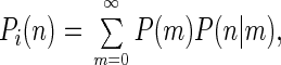1

where P(m) is the Poissonian distribution of the number of molecules with the mean value cdV_i, and c is the concentration of the molecules. P(n|m), which denotes the conditional distribution of the number of photon counts, provided there are m molecules inside the confocal volume, is also a Poissonian distribution with the mean value mqB_iT. Here, q is the specific brightness (count rate per molecule if situated in a “standard” position in which B = 1), and T is the width of the counting time interval. Therefore, the distribution P_i(n) is double Poissonian and has two parameters, cdV_i and qB_iT:

2

Eq. 2 describes ideal solutions of noninteracting molecules at fixed positions during the counting interval T. Therefore, we are justified in applying Eq. 2 for low values of T, where each molecule does not change its brightness significantly because of diffusion.

Note that the distribution of the number of photon counts emitted from the ith section P_i(n) does not depend on the shape of the section. Therefore, one may combine spatial sections of equal B values, even if they are separated by great distances. The three-dimensional function B(r) is reduced to a one-dimensional relationship between B and V, which significantly facilitates numeric calculations.

Assuming given values of B_i and dV_i, one can calculate contributions from different sections P_i(n) and combine them through convolutions. Also, the contribution to the overall distribution P(n) from different species as well as from a constant background may be calculated through convolutions. This calculation scheme is straightforward but clumsy and slow because of a recurrent calculation of convolutions.

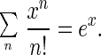
A more convenient representation exists that allows one to express the photon count number distribution explicitly. Also, compared with the calculation of P(n) through convolutions, it is considerably faster. It is the representation of the generating functions. The generating function of a distribution P(n) is defined as

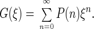3

ξ may in general be a real or a complex argument. If we select ξ = exp(iϕ), then G(ϕ) and P(n) are interrelated through a Fourier transformation. What makes the generating function attractive in photon count number distribution analysis is the additivity of its logarithm; logarithms of generating functions of photon count number distributions of independent sources, like different volume elements as well as different species, are simply added for the calculation of the combined distribution. The substantiation is that the transformation described in Eq. 3 maps distribution convolution into the products of the corresponding generating functions. Applying Eq. 3 to Eq. 2 and leaving out the subscript i for convenience, the contribution from a particular species and a selected volume element dV can be written as

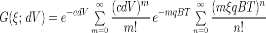4

where we used the following identity twice:

5

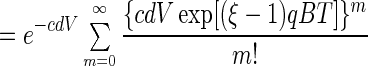
Although P(n) is expressed through convolution integrals, G(ξ) can be expressed by spatial integrals:

6

with index j denoting species here.

Now let us return to the problem of the unknown relationship between B and V. To calculate the spatial integral on the right side of Eq. 6, we may introduce a variable x = ln[B(0)/B(r)] and express dV/dx in terms of x. For numeric calculations, this relationship must correspond sufficiently well to the experimental spatial brightness profile B(r). For a convenient and flexible expression, we use the formula

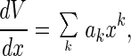7

with only terms k = 1,2,3 included. The values a_kare empirical characteristics of the optical equipment and are determined from adjustment experiments on single species, in a manner similar to that by which moments of the spatial profile are determined in MAFID or as an elongation parameter of the sample is determined in FCS. Because the first two moments of B(r), ∫B(r)dr and ∫B²(r)dr, are usually normalized to unity, there are only two adjustment parameters among three values of a_k and a value of B(0).

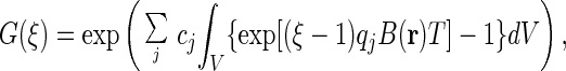
We have realized FIDA in two qualitatively different forms. One may fit the measured distribution P̂(n) assuming a certain number of fluorescent species, and estimate unknown concentrations, c_j, and specific brightness values, q_j. This type of fit is described as a multicomponent fit. Usually, two to five unknown parameters are estimated from a single experiment.

An alternative use of FIDA is inverse transformation realized with the help of linear regularization and constraining concentrations to non-negative values (inverse transformation with regularization is denoted as ITR. For an introduction to ITR analysis, see ref. 9, whereas a more detailed description is given in ref. 10. ITR is used to determine, from the measured P̂(n), the distribution of fluorescent particles with respect to their specific brightness, i.e., it determines for a predefined grid of specific brightness values, q_j, the respective concentrations, c_j. In the output spectrum, negative concentrations are prohibited and ideal δ-peaks of single species are widened by an essential smoothing effect of the ITR method. It is a valuable tool especially for samples either from which too little a priori information about the sample composition is given or in which the sample composition is heterogeneous.

The presented theory is relatively simple and compact because of a number of simplifying assumptions. There are two assumptions that deserve special attention because of their requirements to the conditions of experiments. We have assumed (i) that coordinates of molecules do not change significantly during a counting time interval and (ii) that the brightness of each molecule can be expressed as a product of a spatial brightness function, which is common to all species, and specific brightness, which has a characteristic value for each species. In experiments, both of the assumptions are violated to some extent, with more or less serious consequences. As a modest violation of assumption i, we have selected a counting interval of 40 μs which is 20% of the characteristic diffusion time of Rh6G molecules into and out of the sample volume. By applying assumption i, the apparent brightness of molecules is reduced by 6% compared with the corresponding true value (of immobile molecules), and the apparent sample volume is increased by the same margin. Trapping of molecules into a triplet excited state where they are “invisible” for a short period is a phenomenon known to influence FCS results (11); in FIDA, this phenomenon violates assumption ii and may have more severe consequences than diffusion. In conditions of experiments described below, the apparent brightness of a Rh6G molecule is reduced by 14% compared with its brightness in the singlet state. The shape of the spatial brightness function is also deformed because in-focus molecules spend more time in the triplet state than slightly off-focus molecules. (Molecules exactly in focus spend 18% of their time in the triplet state.) As a consequence of this deformation, the apparent sample volume is increased by 9%. Deformation of the shape of the spatial brightness function causes relatively little harm if different species have similar triplet parameters, because our formula adjusts to the deformed brightness profile. However, if different species have significantly different triplet populations, but the analysis is applied with a single spatial brightness function common to all species, then the result of analysis may be significantly biased. A more sophisticated theory accounting diffusion and triplet trapping is a subject for further studies.

Results and Discussion

In Fig. 1A, the calculated photon number distributions, P(n), are plotted in five different cases. Note that all cases in Fig. 1A correspond to the same mean count rate but to a different composition of the sample; we have selected a lower specific brightness value with a higher concentration value and vice versa. Indeed, a feature vitally important for FIDA is that P(n) depends not only on the mean count rate but selectively on both the concentration and the specific brightness. Another important point is that FIDA can separate the contributions of individual species unambiguously. The filled symbol curve of Fig. 1A corresponds to a mixture of two species; one can visually recognize that this curve is of a different shape than any of the curves calculated for single species.

Figure 1.

Theoretical and experimental distributions of the number of photon counts. (A) Expected probability distributions P(n) for five cases of equal mean count rate, n̄ = 1.0. The open symbols correspond to solutions of single species but with different values of the mean count number per particle qT. The solid line is calculated for a mixture of two species, one with qT = 0.5 and the other with qT = 8.0. (B) Measured distributions of the number of photon counts. The data for three samples are presented: the solutions of 0.5 nM Rh6G, 1.5 nM tetramethylrhodamine (TMR), and a mixture of them (0.8 nM TMR, 0.1 nM Rh6G). The time window of 40 μs was used, and the number of photon counts was determined 1,250,000 times in each of the 50s experiments. (C) Weighted residuals from multicomponent fit analysis of the count number distribution measured for Rh6G. (D) Results of ITR analysis applied to the curves shown in Fig. 1B. The dashed lines correspond to the solutions of single dyes (Rh6G and TMR), and the solid line corresponds to their mixture. The ordinates give the mean number of particles within the confocal volume element (left, single dyes; right, mixture).

In test experiments, we analyzed pure solutions of two different dyes, Rh6G and TMR, as well as a mixture of the two. The primary piece of equipment used routinely for fluorescence correlation studies is a confocal microscope (ConfoCor; EVOTEC BioSystems and Carl Zeiss, Germany). An attenuated (to about 800 μW) beam from an argon ion laser (wavelength 514.5 nm) is focused to a spot with a radius of approximately 0.5 μm, which is twice the size of a spot in usual FCS experiments, and results in a diffusion time of approximately 200 μs for Rh6G. The excitation intensity has generally been kept lower than or equal to a level characterized by about 15% amplitude of the triplet term of the autocorrelation function. Fluorescence emission is detected through a pinhole on the focal plane of the microscope by using an avalanche photodiode detector SPCM-AQ 131 (EG&G, Vaudreuil, Canada).

In Fig. 1B, the distributions of the number of photon counts measured at a dwell time of 40μs and a data collection time of 50 s are presented for Rh6G, TMR, as well as for their mixture. These distributions serve as input data for FIDA. The results of multicomponent fit analysis are given in Table 1 with χ² values calculated according to:

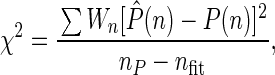8

where n_P is the length of the measured distribution P̂(n), and n_fit is the number of fit parameters. The exemplary residuals for Rh6G are shown in Fig. 1C.

Table 1.

Results of fitting photon count number distributions

Sample	a2	a3	C	q, kHz	χ2
Rh6G	−0.380  ± 0.009	0.077  ± 0.003	0.461  ± 0.003	107.2  ± 0.8	0.97
TMR	−0.427  ± 0.032	0.084  ± 0.014	1.517  ± 0.012	36.56  ± 0.29	0.81
Mixture	−0.380 (fixed)	0.077 (fixed)	0.103  ± 0.012	109.1  ± 4.0	0.77
			0.738  ± 0.011	37.4  ±1.0

In all cases, the background count rate was fixed to the value of 1.05 kHz, as measured with deionized water. a₂ and a₃ are prenormalization values when a₁ is fixed to 1.0. Errors shown are theoretical errors returned by the fitting algorithm multiplied by an empirical factor of three. 

Statistical errors of estimated parameters returned by the fitting algorithm correspond to the theoretical weights:

9

This formula is derived under a simple assumption of N independent measurements of the number of photon counts. In reality, consecutive measurements are correlated; therefore, the errors of estimated parameters returned by the fitting algorithm underestimate real statistical errors. We have determined empirically in a separate series of 30 to 200 measurements that these statistical errors are greater than theoretical ones by a factor of about three. Thus, the errors shown in Table 1 are theoretical errors multiplied by three.

The results of ITR analysis are shown in Fig. 1D, which expresses the distribution of the number of particles as a function of their specific brightness. The ideal outcome would be single δ-peaks for the solutions of single species and two δ-peaks for the mixture. In reality, the width of the ITR output spectral peaks is determined not only by the true width of the distribution of specific brightness values but also by the accuracy of input data and the particular realization of the linear regularization (10); put simply, if a broad spectrum fits experimental data as well as a narrow one then ITR prefers the broad one.

The specific brightness values of Rh6G and TMR differ by a factor of three under our experimental conditions. A good reproduction of the two values of specific brightness from a measurement of the mixture requires relatively long data collection times on the order of tens of seconds. However, if the positions of the peaks are known beforehand, then the corresponding concentrations can be determined much faster.

FIDA opens up new opportunities for the design of fluorescence-based biochemical assays. Among other applications, DNA-DNA interactions can be measured by this new method. The hybridization of oligonucleotides or single DNA strands is of great interest in analyzing particular DNA sequences such as in genome sequencing or cloning projects.

As an example, we applied FIDA to study the hybridization of 5′-(6-carboxytetramethylrhodamine (TAMRA))-labeled 40- mers with either labeled or non-labeled complementary oligonucleotides and the subsequent symmetrical cleavage of the DNA hybrid by the restriction endonucleases HindIII and KpnI. Real-time enzyme kinetics of such cleavage reactions can be followed by dual-color fluorescence cross-correlation spectroscopy (12). This approach, however, does not resolve individual cleavage products. Our approach is designed to illustrate the power of FIDA in resolving the molecular brightness of all fluorescent components within a biological assay system.

The specific oligonucleotides used in this study were TAMRA-AAGAAGGGGTACCTTTGGATAAAAGAGAAGCTTTTCCCGT (5′-TAMRA-Oligo A) and TAMRA-ACGGGAAAAGCTTCTCTTTTATCCAAAGGTACCCCTTCTT (5′-TAMRA-Oligo B). They were purchased in HPLC-pure quality from Applied Biosystems (Weiterstadt, Germany). All measurements were carried out on the FCS reader described above at excitation/emission wavelengths of 543/580 nm by using a 4 mW helium/neon laser (Uniphase, San Jose, CA) attenuated to approximately 300 μW. The water background was measured to be below 800 Hz. For the measurements, sample aliquots were diluted to 1 nM, and 20-μl aliquots were assayed in a 8-well chambered coverglass (Nalge Nunc International, Naperville, IL) at room temperature.

The hybridization reaction was performed in 70% formamide containing 10 mM Tris/HCl buffer (pH 8.0), 1 mM EDTA, 0.2 mM NaCl and an oligonucleotide concentration of 0.5 μM. Denaturation was at 95°C for 2 min and subsequent hybridization was at 55–60°C for 40 min in accordance with the optimized temperature, which is 10–15 degrees below the melting point T_m (Heating block, Techne Laboratories, Princeton). The melting point was calculated as follows: T_m = 81.5 +16.6 (log10[Na⁺]) + 0.41 (%G+C) − 600/N (N = 40; %G+C = 42.5). Restriction digest analyses of the hybrid DNA were performed by the restriction enzymes HindIII and KpnI. The restriction site was chosen to obtain fragments of different size. The cleavage reactions were performed in 3.3 mM Tris-acetate (pH 7.9), 1 mM magnesium acetate, 6.6. mM potassium acetate and 0.1 mg/ml BSA at 37°C for 1h.

The reaction course is characterized by significant shifts of the fluorescence intensity per molecule within a range of one order of magnitude (Fig. 2 A–E). It is important to note that the resulting double product peak corresponds to one single hybridization species in which no nonhybridized species are detectable. This property could be easily shown in hybridization/cleavage experiments by using labeled/nonlabeled oligonucleotide combinations in which signals with brightness values different from the brightness of the double-labeled hybrid have been obtained (Fig. 3 A and B). One explanation for such a double-peak structure could be conformational fluctuations resulting from transitions between two conformational states (13, 14). This behavior is described by using a three-state model of the conformational dynamics with a polar, a nonpolar, and a quenching environment of the label (15). From our data it can be concluded that the conformational fluctuations depend significantly on the DNA length and the number of labels. The small digested DNA fragments have a single brightness, and the concentration ratio of the educt double peaks shifts toward one component when one-label hybrids are studied. As a further result, small fragments show low molecular brightness, and large fragments correspond to high brightness values (Q₂ ≈ Q₃, Q₁ ≈ Q₄).

Figure 2.

ITR analysis of hybridized (A–C) and restriction enzyme-cleaved (D and E) labeled oligonucleotides. All ITR curves are of exemplary nature. They result from a set of 20 individual 10 s measurements which show variations among each other of less than 10%.

Figure 3.

Hybridization and restriction enzyme cleavage of different combinations of labeled and unlabeled oligonucleotides. Restriction digest analyses of the hybrid DNA were performed with the restriction enzymes HindIII and KpnI either alone or in combination. The restriction sites lead to symmetrically cleaved fragments (2x12 mers, 1x16 mer for double digest). The filled circles correspond to labeled DNA. Q_01–03, intensities of DNA hybrids; Q_i, intensities of cleavage products.

Based on symmetrical cleavage sites for both enzymes DNA fragments of equal size and subsequently very similar molecular brightness are to be expected. Fig. 3 A and B clearly illustrates that such a result has been observed, and a relationship, Q₁ + Q₂ = Q₃ + Q₄, is valid. The most important feature of the results of FIDA is that the cleavage products can be identified by the reproducible positions of their peaks in ITR (or, if a multicomponent fit is used, by corresponding specific brightness values of components). For example, a peak at approximately 25 kHz always appears when the initial DNA is labeled at the 5′-end of Oligo B and the enzyme HindIII is used, independently of whether Oligo A was labeled or whether the enzyme KpnI was also used. The bulk of all the measurements of the cleavage products with both single and doubly labeled DNA structures makes it possible to classify all observed intensities with individual structures in a single measurement—a property of FIDA that is not possible with any other known analytical method.

FIDA has a number of striking features. It is one out of few methods enabling the study of single molecules; the concept is simple, and the associated calculations can be performed rapidly in real time. Based on the single-molecule detection nature, the high-intensity resolution, and rapid data acquisition, the system is suitable for high-throughput screening of biologically relevant assays.

Abbreviations

FCS

fluorescence correlation spectroscopy

FIDA

fluorescence-intensity distribution analysis

MAFID

moment analysis of fluorescence-intensity distribution

TAMRA

5′-(6-carboxytetramethylrhodamine)

TMR

tetramethylrhodamine

Rh6G

rhodamine 6G

References

- 1.Mets Ü, Rigler R. J Fluoresc. 1994;4:259–264. doi: 10.1007/BF01878461. [DOI] [PubMed] [Google Scholar]
- 2.Elson E L, Magde D. Phys Rev Lett. 1974;13:1–27. [Google Scholar]
- 3.Magde D, Elson E L, Webb W W. Biopolymers. 1974;13:29–61. doi: 10.1002/bip.1974.360130103. [DOI] [PubMed] [Google Scholar]
- 4.Magde D, Elson E L, Webb W W. Phys Rev Lett. 1972;29:704–708. [Google Scholar]
- 5.Qian H, Elson E L. Proc Natl Acad Sci USA. 1990;87:5479–5483. doi: 10.1073/pnas.87.14.5479. [DOI] [PMC free article] [PubMed] [Google Scholar]
- 6.Qian H, Elson E L. Biophys J. 1990;57:375–380. doi: 10.1016/S0006-3495(90)82539-X. [DOI] [PMC free article] [PubMed] [Google Scholar]
- 7.Evotec Biosystems AG. Int. Patent Appl. PCT/EP97/05619 and Int. Publ. No. WO 98/16814. 1998. [Google Scholar]
- 8.Palmer A G, Thompson N L. Appl Opt. 1989;28:1214–1220. doi: 10.1364/AO.28.001214. [DOI] [PubMed] [Google Scholar]
- 9.Press W H, Teukolsky S A, Vetterling W T, Flannery B P. Numerical Recipes in C: The Art of Scientific Computing. Cambridge, U.K.: Cambridge Univ. Press; 1992. [Google Scholar]
- 10.Biemond J, Lagendijk R L, Mersereau R M. Proc IEEE. 1990;78:856–883. [Google Scholar]
- 11.Widengren J, Mets U, Rigler R. J Phys Chem. 1995;99:13368–13379. [Google Scholar]
- 12.Kettling U, Koltermann A, Schwille P, Eigen M. Proc Natl Acad Sci USA. 1998;95:1416–1420. doi: 10.1073/pnas.95.4.1416. [DOI] [PMC free article] [PubMed] [Google Scholar]
- 13.Edman L, Mets Ü, Rigler R. Proc Natl Acad Sci USA. 1996;93:6710–6715. doi: 10.1073/pnas.93.13.6710. [DOI] [PMC free article] [PubMed] [Google Scholar]
- 14.Wennmalm S, Edman L, Rigler R. Proc Natl Acad Sci USA. 1997;94:10641–10646. doi: 10.1073/pnas.94.20.10641. [DOI] [PMC free article] [PubMed] [Google Scholar]
- 15.Eggeling C, Fries J R, Brand L, Günther R, Seidel C A. Proc Natl Acad Sci USA. 1998;95:1556–1561. doi: 10.1073/pnas.95.4.1556. [DOI] [PMC free article] [PubMed] [Google Scholar]