Prokaryotic Gene Finding Based on Physicochemical Characteristics of Codons Calculated from Molecular Dynamics Simulations

Abstract

An ab initio model for gene prediction in prokaryotic genomes is proposed based on physicochemical characteristics of codons calculated from molecular dynamics (MD) simulations. The model requires a specification of three calculated quantities for each codon: the double-helical trinucleotide base pairing energy, the base pair stacking energy, and an index of the propensity of a codon for protein-nucleic acid interactions. The base pairing and stacking energies for each codon are obtained from recently reported MD simulations on all unique tetranucleotide steps, and the third parameter is assigned based on the conjugate rule previously proposed to account for the wobble hypothesis with respect to degeneracies in the genetic code. The third interaction propensity parameter values correlate well with ab initio MD calculated solvation energies and flexibility of codon sequences as well as codon usage in genes and amino acid composition frequencies in ∼175,000 protein sequences in the Swissprot database. Assignment of these three parameters for each codon enables the calculation of the magnitude and orientation of a cumulative three-dimensional vector for a DNA sequence of any length in each of the six genomic reading frames. Analysis of 372 genomes comprising ∼350,000 genes shows that the orientations of the gene and nongene vectors are well differentiated and make a clear distinction feasible between genic and nongenic sequences at a level equivalent to or better than currently available knowledge-based models trained on the basis of empirical data, presenting a strong support for the possibility of a unique and useful physicochemical characterization of DNA sequences from codons to genomes.

INTRODUCTION

Genome analysis, the problem of finding genes and locating control regions in DNA sequences, has received wide attention in recent years (1–5). Although there is no substitute for molecular biology for determining the exact locations of genes and control sequences in a genome, diverse computational methods (6–22) have been shown to have reasonably successful predictive power. Most of the proposed prediction protocols are based on prior empirical knowledge of sequence characteristics and are thus “knowledge based.” Among the most popular of these involve training on a set of known genic sequences using techniques such as hidden Markov (10,11) or machine learning (13) and have achieved specificities as high as ∼80%. However, the lack of large enough samples of known genes, as typically seen in a newly sequenced genome, can lead to suboptimal level of prediction, and knowledge-based protocols may be organism specific.

In this article we describe an essentially ab initio model for gene prediction in prokaryotic genomes based on a set of three physicochemical characteristics of codons—by codon is meant here the double-helical trinucleotide in DNA space in a given reading frame—calculated from molecular dynamics (MD) simulations. By use of this approach, information on the sequence-dependent properties of genomic segments can be introduced effectively. The resulting gene-finding program, called ChemGenome2 (CG2), is shown to differentiate genes from nongenes at a level equivalent to or better than previously reported gene-finding methods, underlining the possibility of a unique and useful ab initio characterization of DNA sequences from codons to genomes.

BACKGROUND

Gene finding using knowledge-based approaches has been reviewed in the recent comprehensive text by Mount (1), and an updated view has been presented by Ussery and Hallin and others (2–7). Remarkable advances have been made in this area using statistical methods, mathematical models, and artificial intelligence techniques in the design of computational protocols. Further improvements in this general type of approach to gene finding depend on enlarging the database of known genes.

This article is concerned with an alternative approach: ab initio methods based on physicochemical properties and geometrical structures of codons. Some of the changes involved in gene expression are unwinding or melting of DNA helix, interactions with RNA polymerase/transcriptional factors, and short-term interactions with the transcribed RNA molecule. For transcription and replication, base pair opening and DNA unwinding need to occur, which brings into consideration DNA melting and hence relative stability of DNA (gene sequences) vis-à-vis promoter or nongenic regions. In a simple model, stability is attributed to hydrogen bonding between bases and base-stacking interactions. It is also known that stacking energies have been correlated with DNA melting temperature (23). Previous research in this vein has been done by Dutta et al. (24), who developed a simple three-parameter model for gene finding based on Watson-Crick hydrogen bond energies, base-stacking energies, and a protein-DNA interaction parameter. The hydrogen bonding (x dimension) and stacking energies (y dimension) for each codon were assigned based on finite-difference Poisson-Boltzmann calculations, assuming canonical B-form structures. The parameters were taken as a basis for a three-dimensional “j-vector” for each three-base-pair sequence, with the third parameter (z dimension) chosen to give the maximum separation in orientation of summation j-vectors (J-vectors) for genes and nongenes in a training set of 1500 gene/nongene pairs in the Escherichia coli K12 genome. In this regard, the method of Dutta et al. is not purely ab initio but involves a knowledge-based component in the assignment of the z parameter. However, the z parameter is observed to be consistent with the general rule of conjugates proposed earlier, which has a stereochemical basis (25). Dutta et al. calculated j-vectors for all trinucleotides in 331 prokaryotic, 21 eukaryotic, and 18 viral genomes. Summing up, they found J-vectors for gene and nongene regions to be markedly different in orientation, with gene/nongene classification accuracies comparable to those of purely knowledge-based methods. A general specification of the procedure is referred to as the ChemGenome algorithm.

The work of Dutta et al. (24) can be considered a proof of the concept that gene finding based on a physicochemical model of codons is a viable idea. However, there are several possible improvements. One is to introduce the sequence dependence of the solution structures of codons in the x and y parameters, and the second is to render the j-vector approach into a fully ab initio gene-finding tool by reframing the z parameter as representing the propensity of a codon for intermolecular interactions. The problem of the sequence-dependent structures of codons could be approached by crystallographic (26) or NMR structure determination, but a full set of experimental results based on these methods is not yet available. Three base-pair oligonucleotide systems are readily accessible to computational modeling via MD simulations, and force field and simulation protocols have improved to the point that quite accurate results have been obtained. The problem of sequence effects on DNA structure in general has been recently investigated based on MD simulations, and the results can be applied to sequence-dependent structures of codons. Treating the problem in general involves, at a minimum, the study of the sequence-dependent structures of all 10 unique dinucleotide steps. Because each step may be sensitive to the immediate sequence context, a minimal study of the problem requires a consideration of all 136 unique tetranucleotide steps. MD has been applied to this problem by a consortium of researchers who collectively performed 15-ns trajectories on 39 different 15-base-pair DNA sequences in which multiple copies of all the 136 tetranucleotides are represented. This required a total of roughly 0.6 μs of simulation for systems containing ∼24,000 atoms. Details of the MD simulations and analysis of results are presented elsewhere (27,28), and a Web-accessible database of the results is available at http://humphry.chem.wesleyan.edu:8080/MDDNA. Most relevant here is that the MD results on sequence-dependent structures of trinucleotide sequences required for codons can be obtained as a special case of the results on tetranucleotides.

METHODS

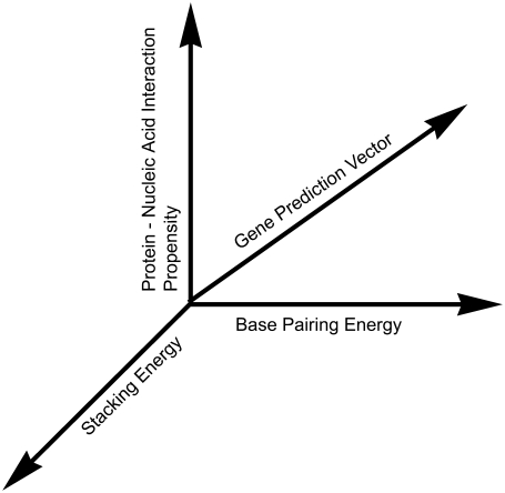
Each of the 64 codons is represented by a three-dimensional j-vector, with each dimension representing a characteristic of DNA structure or recognition as shown in Fig. 1. The x, y, and z components of the j-vector for each codon are nucleotide base-pairing energy, the base pair stacking energy, and an index of the propensity of a codon for intermolecular interactions, each defined on the interval of −1 to +1. The x, y, and z parameters of the j-vector for each codon are listed in Table 1 and are developed as follows.

FIGURE 1.

The three-dimensional physicochemical vector calculated for each DNA sequence.

TABLE 1.

The x (hydrogen-bonding energy), y (stacking energy), and z (protein-nucleic acid interaction propensity parameter) values assigned for each of the 64 codons

Codon	x	y	z	Codon	x	y	z
CCC	−1.0	0.97	−1	TCC	−0.85	0.66	−1
CCG	−0.85	0.14	1	TCG	−0.41	−0.10	−1
CCT	−0.03	1.00	1	TCT	−0.15	0.74	−1
CCA	−0.02	0.81	−1	TCA	−0.18	0.23	−1
CGC	−0.98	−1.00	−1	TGC	−0.49	−0.38	−1
CGG	−0.85	0.14	1	TGG	−0.02	0.81	−1
CGT	−0.30	−0.71	1	TGT	−0.13	0.07	−1
CGA	−0.41	−0.10	−1	TGA	−0.18	0.23	−1
CTC	0.07	0.75	−1	TTC	−0.19	0.50	−1
CTG	0.03	−0.20	1	TTG	0.18	0.26	−1
CTT	0.82	0.87	1	TTT	0.93	0.56	−1
CTA	0.33	0.12	−1	TTA	0.85	0.65	−1
CAC	0.07	−0.25	−1	TAC	0.20	−0.11	−1
CAG	0.03	−0.20	1	TAG	0.33	0.12	−1
CAT	0.15	0.15	1	TAT	0.94	0.41	−1
CAA	0.18	0.26	−1	TAA	0.85	0.65	−1
GCC	−0.90	−0.13	1	ACC	−0.86	0.49	1
GCG	−0.98	−1.00	1	ACG	−0.30	−0.71	−1
GCT	−0.27	−0.24	1	ACT	−0.01	−0.48	−1
GCA	−0.49	−0.38	1	ACA	−0.13	0.07	1
GGC	−0.90	−0.13	1	AGC	−0.27	−0.24	1
GGG	−1.0	0.97	1	AGG	−0.03	1.00	−1
GGT	−0.86	0.49	1	AGT	−0.01	−0.48	−1
GGA	−0.85	0.66	1	AGA	−0.15	0.74	1
GTC	−0.09	−0.01	1	ATC	0.25	0.10	1
GTG	0.07	−0.25	1	ATG	0.15	0.15	−1
GTT	0.57	−0.10	1	ATT	1.0	0.29	−1
GTA	0.20	−0.11	1	ATA	0.94	0.41	1
GAC	−0.09	−0.01	1	AAC	0.57	−0.10	1
GAG	0.07	0.75	1	AAG	0.82	0.87	−1
GAT	0.25	0.10	1	AAT	1.0	0.29	−1
GAA	−0.19	0.50	1	AAA	0.93	0.56	1

Universal plane equation identified for prokaryotes and used for gene prediction in all the 372 genomes studied: n_x = 0.698451, n_y = 6.82635, n_z = 22.8116, d = 1.0.

Hydrogen bond energies (the x component)

The Watson-Crick hydrogen bond energies are calculated from the MD trajectories using ptraj and anal modules of the AMBER software. With the successive bases of a trinucleotide denoted as i, j, and k, and their Watson-Crick partners on the complementary strand as l, m, and n, the hydrogen bond energy is calculated from the simulation data as follows.

where E_i-l refers to the electrostatic plus van der Waals interactions of all the hydrogen-bonding atoms of base i with those of base l. The hydrogen bond energy for all the 32 unique trinucleotides was calculated from all the 39 sequences in the ABC database, and the data were averaged out from the multiple copies of the same trinucleotide. These energies span a range of values from −17.4 kcal mol⁻¹ to −10.7 kcal mol⁻¹. The resultant energies were then linearly mapped onto the [−1, 1] interval giving the x coordinate as

where E[i] is the hydrogen-bonding energy for ith codon, and i ranges from 1 to 64. E_{desired range} here is 2, and E_{desired min} is −1.

Basepair stacking energies (the y component)

The stacking energies, which comprise electrostatic and van der Waals interactions of all the atoms with each other in a codon excluding interactions within the same base pair, were calculated for all 32 unique double-helical trinucleotide sequences in a similar manner.

After averaging out the energies of multiple copies of the same trinucleotide obtained from the MD trajectories, the energies were seen to span the range of −56.2 kcal mol⁻¹ to −52.9 kcal mol⁻¹. The resultant energies were mapped onto the interval [−1, 1], giving the y coordinate for each codon.

where E[i] is the base pair stacking energy for the ith codon, and i ranges from 1 to 64.

Intermolecular interaction propensities (the z component)

Initially for the development of the z parameter (24), we took a training set of 1500 gene-nongene (shifted-gene) pairs (where a gene is at least 100 nucleotides long) of the E. coli K12 genome. These parameters are based on the conjugate rule (25) according to which a codon and its conjugate codon are assigned equal and opposite values (+1 for codon and −1 for its conjugate codon). Codons starting with G are assigned +1. Codons starting with C and ending with G or T are assigned +1, and those ending with A or C −1. The rule of conjugates fixes the remaining 32 values. Conjugate rule extends the wobble hypothesis to capture the general spirit of the molecular events at the recognition site—the dynamics of the third base of the codon on mRNA in the presence of the anticodon.

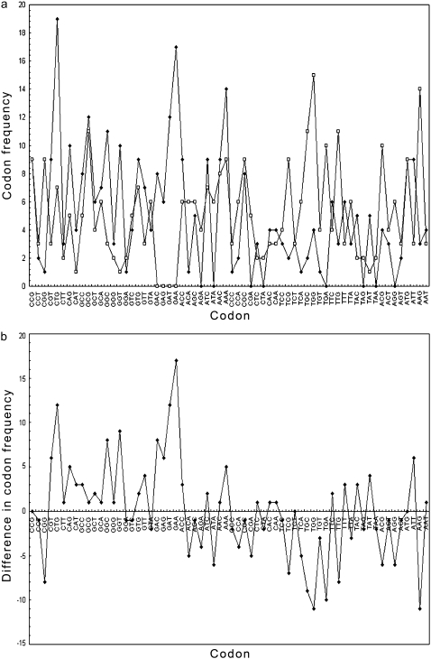
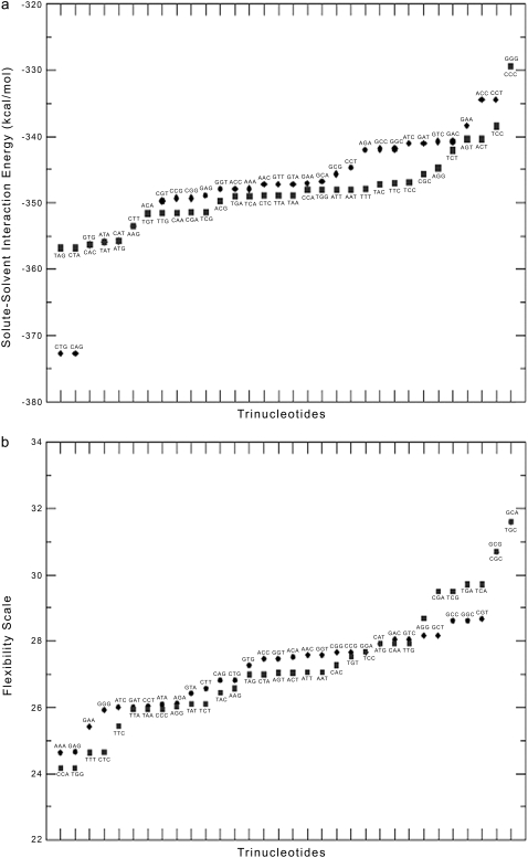
A plot of codon usage (frequency of occurrence of codons) in 854 experimentally verified genes of E. coli (29) is shown in Fig. 2. Note that with the exception of a few, the majority of the codons with +1 value for z have a higher propensity of occurrence in gene sequences compared with those codons with −1 for z, which have a higher propensity for the nongene sequences. The z parameter assignment is found to correlate with the MD calculated solvation energies (Fig. 3 a) and flexibility (Fig. 3 b) of each trinucleotide. The solvation energies of the DNA structural units as observed in the MD simulations were carried out on the basis of the proximity criterion (30), which permits a unique definition of the solution environment of each identifiable substructure—atom, functional group, or residue of any polyfunctional solute molecule or macromolecule (31,32). Specifically, the set of solvent molecules closer to a solute atom A than any other solute atom is referred to as the total primary solvation shell of A. With the proximity indices thus defined for the solute and solvent molecules, the interaction energy between a particular subunit of the solute and the corresponding solvent molecules in its proximity region provides an indicator of the interaction potential. For this analysis, the solute-solvent interaction energies of different trinucleotides of interest were derived on the basis of the MD trajectories. All the proximity analysis calculations presented here have been performed using the MMC program (33), and a detailed analysis of the solvation properties of the various DNA sequences has been reported recently (S. B. Dixit, M. Mezei, and D. L. Beveridge, unpublished data). On average, the trinucleotides with +1 for z have weaker solute-solvent interaction energy (1.1 kcal/mol overall) than their conjugate trinucleotides assigned −1 for z (Fig. 3 a). The flexibility of the different trinucleotide units (Fig. 3 b) has been analyzed on the basis of the average angular mean-square fluctuations in the backbone conformational angles derived from the multiple copies of each trinucleotide unit available in the simulation dataset (28,34). The majority of codons with −1 for z tend to lag behind their conjugate codons assigned +1 in terms of flexibility, although the difference between the averages in this case is small.

FIGURE 2.

(a) Frequency of occurrence of the 64 codons in 854 experimentally verified E. coli genes is presented as black dots, and the corresponding frequency of these codons in the frame-shifted nongenic sequences is presented as open squares. (b) Difference in codon frequencies between genes and nongenes.

FIGURE 3.

(a) The solvation energies of trinucleotides (codons) with +1 for z are presented as diamonds, and those with −1 for z as solid squares. (b) The flexiblity of trinucleotides (codons) with a z value of +1 are presented as diamonds, and those with a z value of −1 are shown as solid squares.

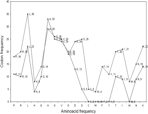
A further analysis of the z parameter (Fig. 4) in terms of Swissprot (35) amino acid composition frequencies observed in 175,000 proteins and the frequency of occurrence of codons that are assigned +1 value in the E. coli dataset mentioned above (29) shows a remarkable similarity. Thus, the z parameter in a sense combines the DNA-protein recognition properties, mRNA-tRNA recognition, and amino acid frequencies in functional proteins. One could envisage a separate set of parameters for each of the above properties, but in CG2, a simple three-dimensional physicochemical model, the z parameter appears to capture the essentials of gene recognition and expression together with x and y.

FIGURE 4.

Correlation between the amino acid frequency in 175,000 Swissprot protein sequences (diamonds) and frequency of occurrence of codons with +1 value for z parameter in the E. coli data set (open squares) for each amino acid.

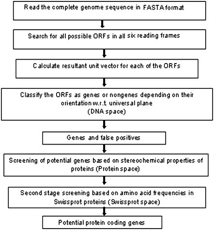
The essential steps involved in gene prediction using CG2 are given in the form of a flowchart in Fig. 5 and, together with Table 1, provide all the information necessary to carry out genome analysis with the CG2 model. To begin the process, a complete genome file is processed for the required format. The genome is then scanned for all possible open reading frames (ORFs) with some minimum length of ORF in all six reading frames. We have currently set the threshold length at 100, although the methodology can work with much smaller lengths. Corresponding to each ORF position, a sequence is extracted from the processed genome file. The physicochemical J-vector is calculated for all the ORF sequences by accumulating the x, y, and z components of the individual codons by vector summation of j-vectors. The orientation of the resultant J-vector is given by the direction cosines. The best universal plane covering the maximum number of genomes with sensitivity greater than 95% is generated using a pocket algorithm (36) and is utilized to segregate these ORF vectors into gene and nongene vectors. The universal plane equation (common to all the 372 prokaryotic systems studied here) is given under Table 1. Irrespective of the species, all vectors lying above this plane are classified as genes, and those below the plane as nongenes (DNA space). These gene vectors include a large number of false positives; however, false negatives are nearly absent.

FIGURE 5.

A flow chart describing the ChemGenome algorithm for gene prediction.

Although the j-vectors for each codon and J-vectors for sequences of codons are purely ab initio, some knowledge-based screening may be applied at a general level to further reduce false positives, i.e., elements that are gene-like but lack promoter sequences and those that are partially mutated to an extent to be incapable of producing functional proteins. One preliminary screen is introduced based on stereochemical properties of protein sequences (protein space) to reduce false positives (B. Jayaram, unpublished data). An analysis of 175,000 Swissprot protein sequences was carried out in terms of the stereochemical properties of the amino acid side chains (linear or branched, hydrogen bond donors, conformationally flexible, and short or long), and it was found that side chains with hydrogen bond donor groups and without branching occur less frequently than the rest. These observations were converted into a computational filter to reduce false positives.

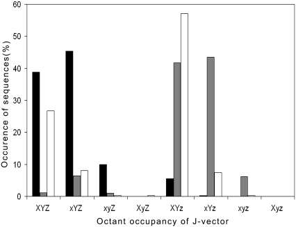
A second screen has also been introduced to reduce false positives based on the frequencies of occurrences of codons via their corresponding amino acids from 175,000 Swissprot proteins. A query nucleotide sequence is converted into amino acids, and their frequency of occurrence is compared with the Swissprot data (Swissprot space). Both the Swissprot amino acid frequency and query nucleotide amino acid frequency are normalized for 100 amino acids, and the difference in the frequencies of Swissprot and query sequence is calculated for each amino acid, as is the overall standard deviation. After validation on a large dataset of experimentally verified genes and nongenes from 372 prokaryotic genomes, we found that a standard deviation (cutoff) of <3.5 captures 95% of genes with 35% of nongenes, whereas a value of <4.0 captures 98% of genes with 47% of false positives. A cutoff of 3.5 is chosen so that the number of false positives is minimum and the precision is maximum. Identification of exact start sites of genes (37) can reduce the false positives in gene prediction considerably. A preliminary attempt is made to map the physicochemical properties of promoter sequences on the basis of j-vector protocol. Fig. 6 shows the octant analysis of mRNA, shifted mRNA (nongenes), and promoter sequences. Promoters dominate in first and fifth octants (i.e., X+, Y+, Z+/Z−), whereas mRNA dominates in first and second octants (i.e., X+/X−, Y+, Z+). A clear difference in octant distribution of the J-vectors for mRNA and shifted mRNA sequences (nongenes) is discernible. However, promoters (regulatory region) and mRNA sequences show a little overlap in the first octant, which needs to be resolved. Work is in progress in this vein. Table 2 and Table S2 in Supplementary Material, Data S1 give the number of ORFs screened after each step along with sensitivity and specificity values.

FIGURE 6.

Octant analysis of DNA sequences. Capital letters on abscissa indicate positive values for the three parameters; small letters indicate negative values. Black bars represent mRNA genes, gray bars represent nongenes (shifted mRNA genes), and white bars represent E. coli promoters.

TABLE 2.

Number of genes predicted and the corresponding sensitivity and specificity at each step in ChemGenome2.0 in the whole genome analyses of 372 prokaryotic genomes

S.No.	NCBI_ID	Initial ORFs	SS	SP	ChemGenome (DNA space)	SS	SP	ChemGenome (protein space)	SS	SP	ChemGenome (Swissprot space)	Annotated gtenes	SS	SP
1	NC_000117	6773	0.99	0.13	4558	0.98	0.19	2135	0.95	0.40	1284	895	0.92	0.64
2	NC_000853	15,104	0.99	0.12	10,688	0.99	0.17	4991	0.97	0.36	3037	1858	0.92	0.57
3	NC_000854	11,774	1.00	0.16	9616	0.99	0.19	5273	0.91	0.32	2282	1841	0.81	0.65
4	NC_000868	11,066	1.00	0.17	6598	0.99	0.28	3524	0.97	0.52	2232	1896	0.90	0.77
5	NC_000907	11,945	1.00	0.14	6582	0.97	0.24	3064	0.93	0.50	1926	1657	0.91	0.78
6	NC_000908	3866	1.00	0.12	1906	0.96	0.24	871	0.85	0.47	491	477	0.81	0.79
7	NC_000909	7829	1.00	0.22	3786	0.99	0.45	2450	0.97	0.68	1488	1729	0.80	0.93
8	NC_000911	28,534	1.00	0.11	20,656	0.98	0.15	10,459	0.95	0.29	5891	3167	0.93	0.50
9	NC_000912	6856	1.00	0.10	3798	0.95	0.17	1331	0.82	0.43	792	689	0.77	0.67
10	NC_000913	41,399	1.00	0.10	30,642	0.99	0.14	15,618	0.97	0.27	8500	4311	0.94	0.48
11	NC_000915	9647	0.98	0.16	5829	0.96	0.26	3227	0.90	0.44	1807	1576	0.86	0.75
12	NC_000916	14,586	1.00	0.13	10,537	0.99	0.18	6315	0.97	0.29	3024	1873	0.91	0.57
13	NC_000917	17,584	0.99	0.14	11,988	0.99	0.20	6121	0.96	0.38	3584	2420	0.90	0.61
14	NC_000918	10,140	1.00	0.15	6591	0.99	0.23	2784	0.98	0.54	1749	1529	0.91	0.80
15	NC_000919	11,875	1.00	0.09	8694	0.99	0.12	4200	0.94	0.23	2165	1036	0.90	0.43
16	NC_000921	9384	0.99	0.16	5682	0.98	0.26	3155	0.92	0.44	1763	1491	0.89	0.75
17	NC_000922	7505	0.99	0.14	5040	0.98	0.21	2484	0.94	0.40	1504	1054	0.91	0.64
18	NC_000961	10,026	1.00	0.19	5869	0.97	0.32	3317	0.94	0.55	2096	1956	0.86	0.80
19	NC_000962	45,751	1.00	0.87	39,813	0.99	0.10	21,629	0.96	0.18	6342	3999	0.85	0.54
20	NC_000963	4307	1.00	0.19	2148	0.97	0.38	1271	0.93	0.61	805	835	0.86	0.89

Data for the first 20 genomes in the order of NCBI IDs are shown in this table. Data for all 372 genomes are provided in Table S2 in Data S1.

RESULTS AND DISCUSSION

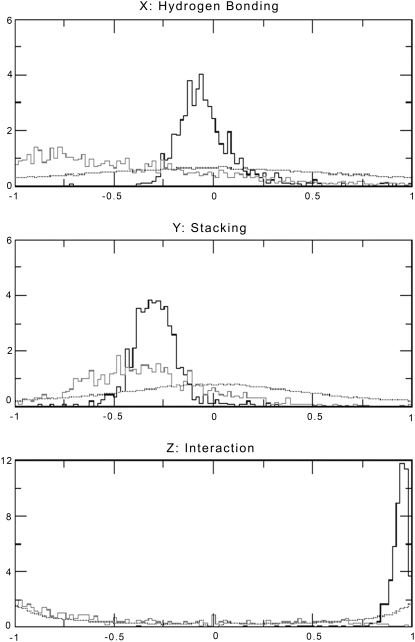
In the CG2 model, each of the 64 codons is assigned a hydrogen bonding, stacking, and interaction propensity parameter based on MD simulation data and the conjugate rule. The values of these three parameters in the cumulative resultant normalized unit vector (the J-vector) are capable of distinguishing genes from nongenes. In Fig. 7, we present the normalized distribution of hydrogen bonding, stacking, and interaction components for 854 experimentally verified genes in the E. coli genome. The frame-shifted nongene sequences derived from these gene sequences as well as a set of 75,000 computationally derived random sequences, each 300 nucleotides long, constitute the reference set of nongene sequences for this analysis. The three graphs highlight the fact that the composition of gene sequences vis-à-vis the nongene and random sequences can be differentiated on the basis of each of the three parameters independently. The combined use of these three parameters in terms of the “J-vector” further improves our ability to differentiate genes from nongene sequences.

FIGURE 7.

Normalized distribution of the (X) hydrogen bond component, (Y) stacking component, and (Z) interaction parameter for 854 experimentally verified genes (black), their corresponding frame-shifted nongene sequences (gray), and 75,000 randomly generated sequences (black dots).

The results of gene finding using CG2 on an already annotated genome with experimentally verified genes are assessed in this study on the basis of true positives (TP, genes identified as genes), false positives (FP, nongenes identified as genes), true negatives (TN, nongenes identified as nongenes), and false negatives (FN, genes identified as nongenes). It is useful to define some derived quantities based on these parameters, viz.

From these quantities the conventional descriptors of assessment can be calculated; i.e.,

where sensitivity refers to the fraction of correct predictions and specificity to the true positive rate. A final assessment parameter for this study, the correlation coefficient, is defined as:

The initial assessment of the CG2 model was carried out on the basis of 372 prokaryotic genomes available in the Genbank (38). The sensitivity, specificity, and correlation coefficients averaged over 356,208 genes and an equal number of frame-shifted genes (nongenes) were found to be 97.5%, 97.20%, and 94.25%, respectively (Table 3 and Table S1 in Data S1). The observed average sensitivity, specificity, and correlation coefficient for gene and pregene (intergenic regions preceeding genes) separation are found to be 92.41%, 82.16%, and 73.30%, respectively (data not shown). The differences in the separation accuracies for gene/shifted gene and gene/pregene may be attributed to the fact that the pregene regions are typically very small in prokaryotic genomes. Usage of a genome-specific plane as opposed to a common (universal) plane for genomes of all species is observed to yield even better accuracies. Overall, the accuracy in the prediction of protein-coding genes in a genome based on a simple three-parameter model capturing the inherent properties of DNA without any prior knowledge of coding regions or database training may be noted.

TABLE 3.

Gene evaluation data for prokaryotic genomes for experimentally verified genes and nongenes

Serial No.	NCBI_ID	Genes	TP	FN	SS	SP	CC
1	NC_000117	455	447	8	0.98	0.96	0.94
2	NC_000853	638	627	11	0.98	0.99	0.97
3	NC_000854	560	544	16	0.97	0.97	0.94
4	NC_000868	619	598	21	0.97	0.98	0.94
5	NC_000907	953	921	32	0.97	0.97	0.94
6	NC_000908	186	182	4	0.98	0.95	0.93
7	NC_000909	713	702	11	0.98	0.98	0.97
8	NC_000911	1351	1298	53	0.96	0.96	0.92
9	NC_000912	238	222	16	0.93	0.93	0.86
10	NC_000913	1914	1217	697	0.64	0.73	0.41
11	NC_000915	731	704	27	0.96	0.96	0.93
12	NC_000916	715	700	15	0.98	0.97	0.95
13	NC_000917	784	774	10	0.99	0.98	0.97
14	NC_000918	594	585	9	0.98	0.98	0.97
15	NC_000919	455	439	16	0.96	0.96	0.92
16	NC_000921	499	488	11	0.98	0.95	0.93
17	NC_000922	619	583	36	0.94	0.95	0.89
18	NC_000961	475	458	17	0.96	0.97	0.93
19	NC_000962	1895	1876	19	0.99	0.99	0.98
20	NC_000963	449	444	5	0.99	0.98	0.97

Data for the first 20 genomes in the order of NCBI IDs are shown in this table. Data for all 372 genomes are provided in Table S1 in Data S1.

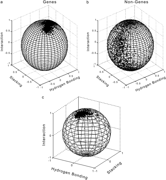
The performance of the model with all the three parameters taken together is shown graphically for the 854 experimentally verified genes (genes where both 5′ and 3′ positions are experimentally verified and function identified) in the E. coli genome as a plot of orientations of predicted cumulated (J) vector over a unit sphere in Fig. 8 a. The clustering of gene vectors (Fig. 8) indicates that genes are characterized by a specific combination of hydrogen-bonding energy, stacking energy, and protein-nucleic acid interaction propensity. For instance, it may be noted from Fig. 6 that genes occur in the first and second octants predominantly. The physicochemical properties of DNA considered in CG2, namely hydrogen-bonding energy and stacking energy together with the z parameter, which correlates with solvation energy and flexibility, seem to embed sufficient information for gene identification. To further gauge the efficacy of the physicochemical model, we deleted all start and stop sites in a genome and tested for gene identification by CG2. The results are shown in Table 4. CG2 identifies gene regions to within ±10 codons with an accuracy exceeding 90%.

FIGURE 8.

(a) Representation of cumulative physicochemical codon vectors on a unit sphere for 854 experimentally verified genes in E. coli and (b) their corresponding frame-shifted nongene sequences. (c) Second view for genes on unit sphere.

TABLE 4.

Accuracy of ChemGenome2.0 in locating the start and stop positions without a prior knowledge of start and stop sites

			Percentage of genes whose start site is identified to within			Percentage of genes whose stop site is identified to within
S.No.	NCBI_ID	Number of experimentally verified genes	±10 bases	±20 bases	±30 bases	±10 bases	±20 bases	±30 bases
1	NC_000117	602	66.0	78.0	83.1	60.8	79.0	85.0
2	NC_000853	1084	91.0	95.0	96.3	87.2	93.1	97.1
3	NC_002570	2143	82.0	90.2	93.3	82.0	89.0	93.0

The CG2 algorithm as described herein has been programmed into a Web-enabled gene prediction software suite that can be accessed at www.scfbio-iitd.res.in/chemgenome/chemgenomenew.jsp. A mirror site has also been created at http://chemgenome.wesleyan.edu. A linux version of the software is also available for free download. A click on the Chemgenome2.0 server opens into a window wherein a user can input the whole genome sequence or a part of the genome of an organism. The sequence can be uploaded or alternatively pasted or typed into the query window of the browser. Acceptable characters are A, G, C, and T. The user can select the minimum ORF length to scan the entire genome. A tabular output displays the strand name and the predicted gene boundaries. A karyogram of the whole genome demarcating protein-coding and noncoding regions is also displayed.

SUMMARY AND CONCLUSIONS

An ab initio model for gene prediction in prokaryotic genomes is proposed based on the assigned j-vectors for each codon and of the orientation of the cumulative J-vectors for a nucleotide sequence element (putative gene). The components of each j-vector correspond to base pair hydrogen bonding, base stacking, and an index representing a propensity for intermolecular interactions. The parameters are calculated from MD simulations and a quantification of the wobble hypothesis. The latter correlates well with MD-calculated solvation energies and flexibility of codon sequences as well as amino acid composition frequencies in ∼175,000 protein sequences in the Swissprot database. Assignment of these three parameters for each codon enables the calculation of the magnitude and orientation of a cumulative three-dimensional vector for a DNA sequence of any length in each of the six genomic reading frames. Analysis of 372 genomes comprising ∼350,000 genes shows that the orientations of the gene and nongene vectors are well differentiated and make a clear distinction feasible between genic and nongenic sequences. Moreover, the success achieved in differentiating genes from nongenes is equivalent to or better than the currently available knowledge-based models trained on the basis of empirical data, presenting a strong support for the possibility of a highly useful physicochemical characterization of DNA sequences from codons to genome.

SUPPLEMENTARY MATERIAL

To view all of the supplemental files associated with this article, visit www.biophysj.org.

References

- 1.Mount, D. W. 2001. Bioinformatics: Sequence and Genome Analysis. Cold Spring Harbor Laboratory Press, Cold Spring Harbor, NY.
- 2.Binnewies, T. T., Y. Motro, P. F. Hallin, O. Lund, D. La, T. Dunn, D. J. Hampson, M. Bellgard, T. M. Wassenaar, and D. W. Ussery. 2006. Ten years of bacterial genome sequencing: comparative-genomics-based discoveries. Funct. Integr. Genomics. 6:165–185. [DOI] [PubMed] [Google Scholar]
- 3.Fickett, J. W. 1996. The gene identification problem: An overview for developers. Comput. Chem. 20:103–118. [DOI] [PubMed] [Google Scholar]
- 4.Claverie, J. M. 1997. Computational methods for the identification of genes in vertebrate genomic sequences. Hum. Mol. Genet. 6:1735–1744. [DOI] [PubMed] [Google Scholar]
- 5.Stormo, G. D. 2000. Gene-finding approaches for eukaryotes. Genome Res. 10:394–397. [DOI] [PubMed] [Google Scholar]
- 6.Mathé, C., M. F. Sagot, T. Schiex, and P. Rouzé. 2002. Current methods of gene prediction, their strength and weaknesses. Nucleic Acids Res. 30:4103–4117. [DOI] [PMC free article] [PubMed] [Google Scholar]
- 7.Zhang, M. Q. 2002. Computational prediction of eukaryotic protein coding genes. Nat. Rev. Genet. 3:698–709. [DOI] [PubMed] [Google Scholar]
- 8.Borodovsky, M. Y., Y. A. Sprizhitskii, E. I. Golovanov, and A. A. Aleksandrov. 1986. Statistical patterns in primary structures of functional regions in the in E. coli genome: III. Computer recognition of coding regions. Mol. Biol. 20:1145–1150. [PubMed] [Google Scholar]
- 9.Borodovsky, M. Y., and J. D. McIninch. 1993. GeneMark: parallel gene recognition for both DNA strands. Comput. Chem. 17:123–153. [Google Scholar]
- 10.Salzberg, S. L., A. L. Delcher, S. Kasif, and O. White. 1998. Microbial gene identification using interpolated Markov models. Nucleic Acids Res. 26:544–548. [DOI] [PMC free article] [PubMed] [Google Scholar]
- 11.Krogh, A., I. S. Mian, and D. Haussler. 1994. A hidden Markov model that finds genes in E. coli DNA. Nucleic Acids Res. 22:4768–4778. [DOI] [PMC free article] [PubMed] [Google Scholar]
- 12.Lukashin, A. V., and M. Borodovsky. 1998. GeneMark.hmm: new solutions for gene finding. Nucleic Acids Res. 26:1107–1115. [DOI] [PMC free article] [PubMed] [Google Scholar]
- 13.Hayes, W. S., and M. Borodovsky. 1998. How to interpret an anonymous bacterial genome: machine learning approach to gene identification. Genome Res. 8:1154–1171. [DOI] [PubMed] [Google Scholar]
- 14.Audic, S., and J. M. Claverie. 1998. Self-identification of protein-coding regions in microbial genomes. Proc. Natl. Acad. Sci. USA. 95:10026–10031. [DOI] [PMC free article] [PubMed] [Google Scholar]
- 15.Baldi, P. 2000. On the convergence of a clustering algorithm for protein-coding regions in microbial genomes. Bioinformatics. 16:367–371. [DOI] [PubMed] [Google Scholar]
- 16.Besemer, J., and M. Borodovsky. 1999. Heuristic approach to deriving models for gene finding. Nucleic Acids Res. 27:3911–3920. [DOI] [PMC free article] [PubMed] [Google Scholar]
- 17.Frishman, D., A. Mironov, H. W. Mewes, and M. Gelfand. 1998. Combining diverse evidence for gene recognition in completely sequenced bacterial genomes. Nucleic Acids Res. 26:2941–2947. [DOI] [PMC free article] [PubMed] [Google Scholar]
- 18.Shmatkov, A. M., A. A. Melikyan, F. L. Chernousko, and M. Borodovsky. 1999. Finding prokaryotic genes by the “frame-by-frame” algorithm: targeting gene starts and overlapping genes. Bioinformatics. 15:874–886. [DOI] [PubMed] [Google Scholar]
- 19.Yada, T., M. Nakao, Y. Totoki, and K. Nakai. 1999. Modeling and predicting transcriptional units of Escherichia coli genes using hidden Markov models. Bioinformatics. 15:987–993. [DOI] [PubMed] [Google Scholar]
- 20.Hannenhalli, S. S., W. S. Hayes, A. G. Hatzigeorgiou, and J. W. Fickett. 1999. Bacterial start site prediction. Nucleic Acids Res. 27:3577–3582. [DOI] [PMC free article] [PubMed] [Google Scholar]
- 21.Delcher, A. L., D. Harmon, S. Kasif, O. White, and S. L. Salzberg. 1999. Improved microbial gene identification with GLIMMER. Nucleic Acids Res. 27:4636–4641. [DOI] [PMC free article] [PubMed] [Google Scholar]
- 22.Besemer, J., A. Lomsadze, and M. Borodovsky. 2001. GeneMarkS: a self-training method for prediction of gene starts in microbial genomes. Implications for finding sequence motifs in regulatory regions. Nucleic Acids Res. 29:2607–2618. [DOI] [PMC free article] [PubMed] [Google Scholar]
- 23.SantaLucia, J., Jr. 1998. A unified view of polymer, dumbbell and oligonucleotide DNA nearest-neighbor thermodymanics. Proc. Natl. Acad. Sci. USA. 95:1460–1465. [DOI] [PMC free article] [PubMed] [Google Scholar]
- 24.Dutta, S., P. Singhal, P. Agrawal, R. Tomer, Kritee, E. Khurana, and B. Jayaram. 2006. A physico-chemical model for analyzing DNA sequences. J. Chem. Inf. Model. 46:78–85. [DOI] [PubMed] [Google Scholar]
- 25.Jayaram, B. 1997. Beyond the wobble: The rule of conjugates. J. Mol. Evol. 45:704–705. [DOI] [PubMed] [Google Scholar]
- 26.Hays, F. A., A. Teegarden, Z. J. Jones, M. Harms, D. Raup, J. Watson, E. Cavaliere, and P. S. Ho. 2005. How sequence defines structure: a crystallographic map of DNA structure and conformation. Proc. Natl. Acad. Sci. USA. 102:7157–7162. [DOI] [PMC free article] [PubMed] [Google Scholar]
- 27.Beveridge, D. L., G. Barreiro, K. S. Byun, D. A. Case, T. E. Cheatham 3rd, S. B. Dixit, E. Giudice, F. Lankas, R. Lavery, J. H. Maddocks, R. Osman, E. Seibert, H. Sklenar, G. Stoll, K. M. Thayer, P. Varnai, and M. A. Young. 2004. Molecular dynamics simulations of the 136 unique tetranucleotide sequences of DNA oligonucleotides. I. Research design and results on d(CpG) steps. Biophys. J. 87:799–813. [DOI] [PMC free article] [PubMed] [Google Scholar]
- 28.Dixit, S. B., D. L. Beveridge, D. A. Case, T. E. Cheatham 3rd, E. Giudice, F. Lankas, R. Lavery, J. H. Maddocks, R. Osman, H. Sklenar, K. M. Thayer, and P. Varnai. 2005. Molecular dynamics simulations of the 136 unique tetranucleotide sequences of DNA oligonucleotides. II: Sequence context effects on the dynamical structures of the 10 unique dinucleotide steps. Biophys. J. 89:3721–3740. [DOI] [PMC free article] [PubMed] [Google Scholar]
- 29.Rudd, K. E. 2000. EcoGene: a genome sequence database for Escherichia coli K-12. Nucleic Acids Res. 28:60–64. [DOI] [PMC free article] [PubMed] [Google Scholar]
- 30.Mehrotra, P. K., and D. L. Beveridge. 1980. Structural analysis of molecular solutions based on quasi-component distribution functions. Application to [H2CO]aq at 25 °C. J. Am. Chem. Soc. 102:4287–4294. [Google Scholar]
- 31.Mezei, M., and D. L. Beveridge. 1986. Structural chemistry of biomolecular hydration: the proximity criterion. Methods Enzymol. 127:21–47. [DOI] [PubMed] [Google Scholar]
- 32.Mezei, M. 1988. Modified proximity criteria for the analysis of the solvation of a polyfunctional solute. Mol. Simul. 1:327–332. [Google Scholar]
- 33.Mezei, M. 2006. MMC: Monte Carlo Program for Computer Simulation of Molecular Solutions. Available from: Mihaly.Mezei@mssm.edu.
- 34.Dixit, S. B., S. Y. Ponomarev, and D. L. Beveridge. 2006. Root mean square deviation probability analysis of molecular dynamics trajectories on DNA. J. Chem. Inf. Model. 46:1084–1093. [DOI] [PubMed] [Google Scholar]
- 35.Swiss-Prot Protein knowledgebase. Available at http://ca.expasy.org/sprot/.
- 36.Gallant, S. I. 1990. Perceptron-based learning algorithm. IEEE Trans. Neural Netw. 2:179–191. [DOI] [PubMed] [Google Scholar]
- 37.Yada, T., Y. Totoki, T. Takagi, and K. Nakai. 2001. A novel bacterial gene-finding system with improved accuracy in locating start codons. DNA Res. 8:97–106. [DOI] [PubMed] [Google Scholar]
- 38.Genbank. Available at ftp://ftp.ncbi.nih.gov/genomes/Bacteria/.
Associated Data
This section collects any data citations, data availability statements, or supplementary materials included in this article.