Significance Analysis of Spectral Count Data in Label-free Shotgun Proteomics^,

Abstract

Spectral counting has become a commonly used approach for measuring protein abundance in label-free shotgun proteomics. At the same time, the development of data analysis methods has lagged behind. Currently most studies utilizing spectral counts rely on simple data transforms and posthoc corrections of conventional signal-to-noise ratio statistics. However, these adjustments can neither handle the bias toward high abundance proteins nor deal with the drawbacks due to the limited number of replicates. We present a novel statistical framework (QSpec) for the significance analysis of differential expression with extensions to a variety of experimental design factors and adjustments for protein properties. Using synthetic and real experimental data sets, we show that the proposed method outperforms conventional statistical methods that search for differential expression for individual proteins. We illustrate the flexibility of the model by analyzing a data set with a complicated experimental design involving cellular localization and time course.

MS-based shotgun proteomics is currently the most commonly used approach for the identification and quantification of proteins in large scale studies (1, 2). A variety of mass spectrometry-driven protein quantification methods have been proposed involving stable isotope labeling of proteins or peptides coupled with MS/MS sequencing, e.g. ICAT (3), stable isotope labeling by amino acids in cell culture (SILAC) (4), and multiplexed quantitation using isobaric tags for relative and absolute quantitation (iTRAQ) (5) (for reviews, see Refs. 6 and 7). The well known limitations of label based-methods include requirements for higher amounts of starting biological material, increased complexity of the experimental protocols, and high costs of reagents (7).

As a result, in recent years, so-called label-free methods have received increasing attention as promising alternatives that automatically waive some of the disadvantages of using stable isotope labeling methods. Popular methods in this area have focused on the analysis of two-dimensional images of ion intensities in the span of retention time and m/z from a LC-MS or LC-MS/MS run where peak intensities are used as the abundance measure (8–11). Despite the rich information contained in the LC-MS data, daunting computational effort needs to be spent on processing the data, including background filtering, peak detection, and alignment (8, 11).

A viable label-free quantitative strategy is spectral counting where the number of spectra matched to peptides from a protein is used as a surrogate measure of protein abundance. Although conceptually simple, recent studies have demonstrated that spectral counting can be as sensitive as ion peak intensities in terms of detection range while retaining linearity (12–20). A number of groups have proposed various types of normalized scores based on transformed spectral counts, including methods that explore weighted scoring by peptide match score (16), normalization by the number of potential peptide matches (17), peptide sequence length, overall experiment-wide abundance (18), or incorporation of the probability of identification into counting (19). Standard statistical tests could also be applied on the raw/transformed counts to analyze the protein expression data (20–22).

Despite published examples of using spectral counting in proteomics, there is a lack of computational and statistical methods for analyzing this type of data that are as well established as the counterparts in gene expression data. These include differential expression analysis such as significance analysis of microarray data (SAM) (23), clustering and classification, and network analysis (24–26). Most studies demonstrating the use of spectral counts have resorted to data-driven corrections of conventional signal-to-noise ratio statistics such as mean-variance model adjustment (27) and detection rate adjustment (20). These adjustments are primarily used to correct the bias in the statistic that favors large differences in highly abundant proteins. However, the technical challenges for modeling quantitative proteomics data are distinct in their own right. First neither ion peak intensity extraction nor spectral counting generates data that can easily be modeled with standard distributional assumptions as with gene expression data sets. This increases the burden of finding the appropriate statistical model and estimation methods. Second because of the limited amount of sample material available or MS instrument availability considerations, comparative profiling of two or more distinct biological conditions is rarely performed in sufficient number of replicates or samples. Lacking the opportunity to observe consistent evidence over multiple samples in homogeneous biological condition makes it difficult to perform robust estimation and inference on model parameters. Unless there are more than four or five replicates generated for each condition permutation-based methods for generating reference distributions will not work well.

Here we propose a general statistical framework for analyzing spectral count data. This method addresses the issue of the appropriate probability distribution for count data as well as tackles the paucity of information due to the absence of replicate samples. The model is based on the use of hierarchical Bayes estimation of generalized linear mixed effects model (GLMM)1 (28) where the spectral counts are considered to be random numbers from a large population of proteins, and hence the model parameters are directly shared within replicates and across proteins. This comprehensive modeling strategy is bound to be more powerful than calculating the signal-to-noise ratio type of differential expression test statistics. These are performed on a per protein basis and referenced to an approximate null distribution especially when the number of replicates is limited.

This report is organized as follows. First the overall modeling framework and its applicability to a wide variety of experimental designs is explained, and its advantages are discussed. Then the performance of the proposed method using synthetic data sets is illustrated with a comparison with methods using signal-to-noise ratio statistics. The comparison focuses on the power to detect differentially expressed proteins at fixed error rates and the property of the detected proteins such as abundance. For a real data analysis example, the experimental data set taken from Pavelka et al. (27) comparing proteome profiles of a yeast strain at two different phases in cell growth is reanalyzed. The enrichment analysis compares the biological functions highlighted by the protein signature detected by the proposed method with the conventional signal-to-noise method, and related computational and statistical issues are discussed. Finally using the published data set of a system-wide survey of the mouse proteome in congestive heart failure (29) the proposed methodology is demonstrated in the presence of experimental design factors. Further discussion of potential improvements on the model and possible extensions concludes the report.

EXPERIMENTAL PROCEDURES

Experimental Data Sets

Three data sets were obtained from two published studies (27, 29). In all cases, no reanalysis of the raw MS data was performed in this work, i.e. the spectral count data were taken as reported in the supplemental materials provided in those publications. A brief description of the data sets is given below.

Yeast Control Data Set—

First Pavelka et al. (27) provided a data set containing four biological replicates of BY4741 strain of yeast grown in media enriched with different nitrogen isotopes (¹⁴N and ¹⁵N). Growing yeast in these two different media is not expected to result in differences in protein expression between these two samples. For each growth condition and each replicate, the LC-MS/MS analysis was performed on 500 μg of protein extract. Proteins were TCA-precipitated, urea-denatured, reduced, alkylated, and digested with Lys-C followed by trypsin digestion. The resulting peptide mixtures were separated using a 12-step multidimensional protein identification technology analysis. MS/MS spectra were collected on an LTQ linear ion trap mass spectrometer (ThermoFinnigan) equipped with a nano-LC electrospray ionization source. Each full MS scan was followed by five MS/MS scans using data-dependent acquisition with the dynamic exclusion option specified as follows: repeat count, 1; repeat duration, 30 s; exclusion duration, 300 s. The peak lists were extracted from RAW files using the extract_ms.exe program with default parameter settings (consecutive scans acquired on the same peptide ion grouped into a single .dta file). The resulting peak lists were searched using SEQUEST against a yeast protein sequence database appended with decoy sequences. Protein level summaries were generated using DTASelect with SEQUEST score thresholds set to achieve a less than 1% false protein identification error rate based on decoy counts. The spectral count for each protein was calculated as the number of .dta files assigned a peptide from that protein with high SEQUEST scores passing DTASelect filtering criteria. In total, the data set contains four technical replicates for each of the two growth conditions (light and heavy isotope media) with 1307 proteins identified at least once in the eight analyses. This data set was used as a control data set for simulation studies.

Yeast Comparative Growth Data Set—

The second data set was also taken from Pavelka et al. (27) and represents four biological replicates of the same BY4741 yeast strain grown up to two different stages of cell growth, namely log and stationary phases. MS/MS spectra were collected and processed as described above. This data set contains 1856 unique proteins identified in any of the eight experiments (four replicates for each of the two growth phases). This data set exhibits a significant difference in protein expression levels between the log and stationary phase and was used in this study for the comparison of functional annotation in a real data analysis scenario.

Mouse Data Set—

The third data set was taken from a published mouse study on the causative effect of impaired calcium ion handling that leads to dilated cardiomyopathy and eventual death (29). Organellar protein fractions (mitochondrial, microsomal, and cytosolic) were extracted from pooled ventricle tissue and separated using centrifugation. 100 μg of protein extract was used in each LC-MS/MS experiment, TCA-precipitated, denatured, reduced, alkylated, and digested sequentially with Lys-C and trypsin. The peptide mixtures were separated using a 12-step multidimensional protein identification technology analysis followed by MS/MS sequencing on an LTQ mass spectrometer equipped with an electrospray ion source. Precursor ions were subjected to data-dependent sequencing with dynamic exclusion enabled (one scan, no repeats, exclude for 90 s). The peak lists (.dta files) were extracted from RAW instrument files using extract_ms.exe with default parameter settings. The peak lists were searched using SEQUEST, and the search results were processed using the STATQUEST analysis program. The spectral count for each protein was calculated as the number of .dta files assigned a peptide from that protein with high confidence. The spectral count profiles of 6190 proteins in phospholamban mutant PLN R9C and wild type mice were compared at three time points in cytosol, microsome, and mitochondria. For each combination of time point and organelle, the spectral count profiles of the mutant and the wild type were paired, adding up to 18 spectral count profiles in total.

Simulation Data Sets

Using the first yeast data set described above, two groups of synthetic data sets were generated. Because the original cell cultures were grown in ¹⁴N- and ¹⁵N-media and then mixed into four pools at a 1:1 ratio before LC-MS/MS analysis, in effect these data had no real signals between the two groups in all proteins. To create synthetic data sets with non-trivial differential expression, the rows of the data matrix (proteins) were shuffled to ensure that the distribution of high and low abundance proteins is uniform across the rows. Then the first 200 proteins in the matrix were selected, and 2-fold changes were inserted to the selected proteins, generating the first synthetic data set (F2). The second synthetic data set (F4) was generated by inserting 4-fold changes to the selected proteins. Inserting a fixed -fold change has been achieved on a protein-by-protein basis. Counts in the replicates grown in ¹⁴N-medium were multiplied by the -fold change if the mean count in the four replicates in ¹⁴N-medium was greater than the mean count in ¹⁵N-medium and vice versa. If a count in the group with smaller mean was 0, a randomly generated Poisson random count was inserted with mean equal to the -fold change itself on the opposite group to bypass the null effect of multiplying 0 by the -fold change.

To investigate the effect of the number of replicates on the power of detecting differentially expressed proteins, additional variants of the two data sets described above were derived by varying the number of replicates used: F2-1rep (taking first replicate for each condition), F2-2rep (taking the first two replicates), and F2-3rep (taking the first three replicates). The same was performed with the 4-fold change data set to form subsets F4-1rep, F4-2rep, and F4-3rep, respectively. For the sake of consistency, the original data with all four replicates for each condition (growth media) were named F2-4rep and F4-4rep, respectively (data provided in supplemental Table 1). In addition, the aggregated counts across the four replicates within each condition were computed and saved as two columns of count sums (F2-sum and F4-sum). This last variant was generated to understand whether generating replicates helps by adding more signals to the total signal or by providing any direct information on the variability across replicates.

Functional Annotation

Interpretation of data was assisted by two annotation tools, FATIGO+ (30) and DAVID (31). These tools were used to assign significantly enriched functional categories to a selected set of proteins. FATIGO+ takes the set of target proteins and the set of background proteins, compares the enrichment of each functional category in the two sets, and reports the statistical significance of enriched functions in the former list. DAVID performs essentially the same operation with the option of specifying the background proteins as the complement of the target protein list among all proteins identified in the particular experiment or as the complement in the population of all known proteins in the public databases. FATIGO+ was utilized wherever the “background” list was well defined, and DAVID was used when it was otherwise.

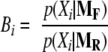
Bayes Factors

A quantity called Bayes factor (32) was used as an indicator of statistical significance of the model parameters, e.g. regression coefficients for differential expression. Bayes factors are essentially likelihood ratios of two competing statistical models where the likelihood of each competing model is averaged over all possible parameter values by numerical integration. Suppose that we observe data X, and we have two models M₁ and M₂ that can describe the observation of X. For each model, we have parameters θ₁ and θ₂, respectively. Then for i = 1 and i = 2, one can calculate the averaged likelihood.

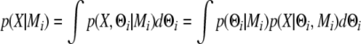1

The Bayes factor is now defined as the ratio of the two averaged likelihoods.

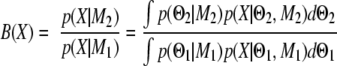2

A large Bayes factor supports the second model M₂ over M₁ for describing the data X. If M₂ is a model with a differential expression coefficient and M₁ is a model without it, a large B indicates statistically significant differential expression.

False Discovery Rate (FDR) Estimation

The rate of false positives in the selection of differentially expressed proteins based on Bayes factors can be estimated using a mixture model-based method of local FDR control (33, 34). Given a log transformed Bayes factor B, the local FDR (denoted as fdr) can be calculated according to Equation 3,

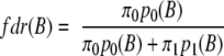3

where p₀(B) and p₁(B) are the proteome-wide distribution of Bayes factor for proteins with trivial and significant differential expression, respectively, and π₀ and π₁ are the corresponding proportion of proteins. Using this method, one can choose a minimum threshold Bayes factor B* that controls the global FDR at a target rate of ∼5% as follows.

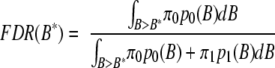4

RESULTS

Statistical Model for Spectral Counts—

For a data set with n samples and p proteins, a model-based method is proposed to select proteins whose absolute abundance changes by a statistically significant amount under different biological conditions. The MS/MS spectral counts of a protein are modeled as observations from the Poisson distribution. This represents a natural choice reflecting the stochastic nature of the peptide sampling process by the mass spectrometer. Similar assumptions are often made in related applications, e.g. in the serial analysis of gene expression (SAGE) approach (35). The expected counts are modeled as a linear function of normalizing factors, treatment or disease status, and other experimental information. Unlike in gene expression data sets, typical proteomics data sets have data over only a few replicates or samples, and as a result, fitting a Poisson regression model for individual proteins separately is often not feasible. The limited sample size can be as restrictive as the example in Fig. 1A, which shows the partial spectral count table for a data set with n = 2.

Fig. 1.

Generalized linear mixed model with hierarchical Bayes for the analysis of spectral count data. The expected counts are normalized by the sequence length of the protein i and the normalizing constant equivalent to the overall abundance of each MS/MS experiment j. In the main text, the sequence length and the normalizing constant are denoted by L_i and N_j, respectively. c₀ is the base-line abundance, and b_0i and b_1i are the protein-specific abundance and differential expression parameters for protein i. Experiment Design Factors may include any discrete levels by which the expected counts may vary, e.g. time points, subcellular localization, etc. A, a subset of the spectral count data matrix without design factors and replicates. B, a subset of the spectral count data matrix with time course and subcellular localization factors. wk, weeks.

To address the challenge of small numbers of replicates, we utilize a statistical methodology called hierarchical Bayes that pools the statistical information on the regression models across proteins. Considering each protein as a member of the population of all identified proteins, we model the regression parameters for each protein as random effects. The random effect terms are the coefficients shared by the replicates within the same protein, allowing one to account for the intrasubject correlation of the data. The random effect terms for the base-line abundance of a particular protein are shared by every sample, and those for the treatment or disease status are shared by the replicates within the same condition.

More specifically, the analysis starts with the observed spectral count data matrix X = [X_ij]. Assuming that X_ij are observations from a Poisson distribution with expected count μ_ij for i = 1, 2, …, p, the expected count matrix is expressed as a GLMM,

5

where μ_ij is the expected count for protein i in replicate j, L_i is the sequence length of protein i, N_j is the normalizing constant of replicate j, c₀ is the base-line abundance, and b_0i and b_1i are the protein-specific abundance and differential expression parameters for protein i. Most importantly, the treatment effect is defined as follows: T_j = 1 if replicate j is in treatment and T_j = 0 otherwise. The first term on the right-hand side of Equation 5 is a fixed normalizing term often referred to as the “offset” in regression analysis. The protein sequence length L_i adjusts for the bias in the count for longer proteins, and the normalizing constant N_j of replicates adjusts for the overall abundance of each replicate or sample (18). For N_j, we use the average count across all identified proteins in sample j to reflect the total abundance of all proteins identified in each MS/MS experiment.

If the treatment effect b_1i is not a statistically significant term, then the model in Equation 5 reduces to the following.

6

The full model (M_F) is denoted in Equation 5, and the reduced model (M_R) is denoted in Equation 6. If the evidence from the spectral count data supports M_F over M_R, the protein is considered as differentially expressed. If the protein is indeed differentially expressed, comparing the goodness of fit by M_F and M_R leads to the selection of differentially expressed proteins. This is because the model with the differential expression parameter fits the data better than the model without it. The exact protein selection method will be described in the next section more precisely.

Given the model setup, the probability distribution for the model parameters are specified as follows. Because M_R is a nested model of M_F, it suffices to write the model specification for M_F. Although the expected spectral counts are expressed in the form of a GLMM, the connection across the model parameters in different proteins has yet to be established. To this end, assume the following.

7

This framework is called hierarchical Bayes because the set of parameters {b_0i} and {b_1i} for all proteins i = 1, 2, …, p are specified as random variables from the Gaussian distribution with inverse γ-distributed variance parameters. Inverse γ distribution refers to the distribution of the reciprocal of the γ random variable with certain shape and scale parameters. Also it is a “conjugate” prior distribution in the sense that the posterior distribution is also an inverse γ distribution. The hierarchical structure in the model specification is known to result in shrinkage estimates that have better statistical properties. This provides the basis for more robust statistical estimation and inference procedures by pooling statistical information across all identified proteins (24), which tends to be helpful in small sample problems. The good property of information pooling has been a well established practice in gene expression data analysis (24, 36). Model parameters are estimated by sample averages of the posterior output from Markov chain Monte Carlo (26, 37) (see supplemental methods for more specific details on the estimation procedure).

Tests for Differential Expression and Multiple Testing Correction—

The strategy for determining whether each protein is differentially expressed between the two conditions is straightforward. For each protein, the Bayes factor (32) was calculated as follows.

8

In Equation 8, the numerator and the denominator are essentially the likelihoods of observing the counts under M_F and M_R, respectively. Thus if this ratio is large, the data support the model with the differential expression parameters over the model without, providing probabilistic evidence that the protein is differentially expressed (see “Experimental Procedures” for details).

Conventionally a Bayes factor greater than 10 suggests a strong evidence for the model in the numerator, and a Bayes factor greater than 30 suggests a very strong evidence for the same model (32). However, these conventional cutoffs may not work efficiently in the high throughput data sets, and appropriate cutoffs have to be chosen in a way that the overall global error is controlled to a desired level. In this work, the distribution of Bayes factors with significant differential expression is discriminated from that without by mixture modeling (see “Experimental Procedures” for details).

Solely applying the Bayes factor threshold, however, does have its own potential drawbacks when there are low quality replicates. Empirically the Bayes factor can be overestimated because of the heterogeneity of counts across replicates rather than the real differential expression. This is especially true for extremely high abundance proteins. In this case, the averaged likelihood in the model without the differential expression parameter (M_R) tends to be penalized more than the model with the parameter (M_F). To address this issue, the selected proteins were required to have a -fold change of no less than 50%. In the subsequent data analysis, of the proteins filtered by this step a small number were found to be in the high abundance range.

Simulation Study—

To assess the performance of the proposed method, it was compared with the conventional signal-to-noise ratio statistics coupled with FDR control. Particularly the variance adjustment of t-statistics by the power law global error model (PLGEM) was reported to have improved the detection of differentially expressed proteins in Pavelka et al. (27); hence that method (PLGEM-StN) was used in place of the conventional t-statistic.

The analysis was performed using a set of synthetic data sets containing 200 proteins with either 2- or 4-fold change embedded in the much large list of proteins identified in the comparative analysis of two biological replicates of yeast (grown in ¹⁴N- and ¹⁵N-media) with no differential expression expected between the replicates (see “Experimental Procedures” for details). The analysis was repeated for data sets containing a varying number of replicates for each of the two conditions (between one and four replicates). The raw spectral counts were converted into normalized spectral abundance factors (27), and the PLGEM-StN model of Pavelka et al. (27) was used to calculate moderated t-statistics and their associated FDR-adjusted p values. The proteins were selected using various cutoffs to examine the power over a wide range of FDRs.

Using the outputs from the two methods, PLGEM-StN and the hierarchical Bayes method (referred to as QSpec from here on) presented here, the comparisons were made based on the power of detection at a fixed FDR. Importantly because the signal-to-noise ratio statistics require the calculation of variance, methods like PLGEM-StN (27) cannot be applied to data sets that have less than three replicates. Therefore the PLGEM-StN analysis was performed for 2- and 4-fold data sets with three or four replicates only, F2-3rep, F2-4rep, F4-3rep, and F4-4rep, respectively. Because the QSpec model does not have this limitation, it was applied on all data sets.

Fig. 2 illustrates the comparison using the synthetic data sets with 2-fold change (Fig. 2, A and B) and 4-fold change (Fig. 2, C and D), respectively. Several trends are apparent. With both methods, PLGEM-StN and QSpec, increasing the number of replicates leads to the selection of a higher number of differentially expressed proteins. Also with the number of replicates fixed, both models are more successful at detecting proteins having higher -fold change (compare corresponding 4- versus 2-fold curves for QSpec and PLGEM-StN models, Fig. 2, A versus C and B versus D, respectively). Comparing the two methods with each other when applied to the same data set, QSpec outperforms the PLGEM-StN across the entire range of FDR values (compare Fig. 2, A versus B and C versus D, for 2- and 4-fold data, respectively). For example, in the F2-4rep data set, QSpec selects 50 proteins (25%) at an FDR of 10%, whereas PLGEM-StN selects only 24 proteins (12.5%). In the F4-4rep data set, QSpec collects 193 proteins (96.5%) at the same FDR level, whereas the other method selects 167 (83.5%). Furthermore the QSpec protein selection from the single replicate data sets, F2-1rep, performs no worse than the PLGEM-StN selection from the three-replicate F2-3rep data set. Similarly the QSpec results in the two-replicate F4-2rep data set are equivalent to the PLGEM-StN results in the three-replicate F4-3rep data.

Fig. 2.

The number of true positive proteins (from the total of 200) identified by QSpec and PLGEM-StN at fixed FDRs in synthetic data sets with known -fold changes and using different number of replicates. A, QSpec, 2-fold change. B, PLGEM-StN, 2-fold change. C, QSpec, 4-fold change. D, PLGEM-StN, 4-fold change. rep, replicate(s).

As an important feature of the model, QSpec performed equally well when applied to the aggregate data sets, F2-sum and F4-sum (with spectral counts from all replicates summed and represented as a single number), as with the original four-replicate F2-4rep and F4-4rep data sets (data not shown). This can be explained by the fact that all the information used to fit the Poisson model is summarized in the count sum (sufficient statistic). More precisely, the Poisson model assumes that the expected count is equal to the variability of the counts (variance) due to its parameterization, so the model does not have a separate variance parameter. The consequences of this inherent assumption are further discussed later.

Because it was found that the real signals accumulate through replicates, the properties of proteins that could not be detected as differentially expressed in the synthetic data sets with only one or two replicates were investigated. One would expect that the area where the gain in statistical power due to replicates is most significant is among low abundance proteins. The ratio of biological signal to the technical noise in low abundance proteins tends to be too low to be accurately characterized using spectral counts in a single shotgun proteomics experiment. Fig. 3 shows the proportion of proteins selected by QSpec among the 200 proteins with spiked signals in the synthetic data sets. Indeed the protein selection achieves greater power in the low abundance range as more replicates are collected and is especially noticeable in the case of proteins with 2-fold change (Fig. 3A).

Fig. 3.

The proportion of true positive proteins (sensitivity of identification) identified by QSpec in the synthetic data sets with 2-fold change (A) and 4-fold change (B) across the range of protein abundance. (x–y) implies counts ranging from x to y. Rep, replicate.

Comparative Growth Analysis—

With the evidence that QSpec outperforms the method of conventional signal-to-noise ratio statistics in simulated settings, the data set from the comparative growth phase analysis (27) was reanalyzed. Before applying QSpec, the distributions of spectral counts in each replicate were analyzed for homogeneity. The spectral counts for one of the replicates (LP3) were vastly higher in many midabundance proteins and lower in low and high abundance proteins relative to other replicates (see supplemental Fig. 1). The degree to which this replicate differed from the others was deemed more than what can be corrected by normalization procedures. For this reason, this replicate was expected to introduce unnecessary heterogeneity in the group logarithmic phase. Therefore, it was removed, and the analysis proceeded with the total of seven replicates. The final data set contained 1508 proteins including 10 contaminants that were excluded from the subsequent analysis.

Analysis with QSpec resulted in the selection of 298 proteins with a Bayes factor above 9.8 (see supplemental Table 2 for details of the analysis). Considering all proteins satisfying this criterion as differentially expressed would introduce on average a 5% or less FDR according to the mixture model-based error estimation (see supplemental Fig. 2). Of the 298 proteins, 121 were overexpressed in the stationary phase, and 177 were overexpressed in the log phase. The GO annotations and their significance measures were given by FATIGO+, and the most significant terms (FDR-corrected p value less than 0.05) located in a reasonably high hierarchy of the GO are shown in Fig. 4A (also see supplemental Table 3 for the entire enrichment analysis results). For comparison, Fig. 4B shows the results of the original analysis presented in Pavelka et al. (27).

Fig. 4.

Venn diagram of the selected proteins from QSpec with all 1508 proteins and PLGEM-StN with the subset of 511 proteins (27). Tables A and B correspond to the significantly enriched gene ontology terms in the protein list identified by QSpec and PLGEM-StN, respectively.

It should be noted that in that work the PLGEM-StN method was applied not to the entire data set of all protein identifications but to the selected subset of 511 proteins that were identified in both the logarithmic and stationary phases. Subsequently the set of 100 proteins with the highest signal-to-noise ratios was selected and categorized using gene ontology of which 34 were overexpressed in the stationary phase and the remaining 66 were overexpressed in the log phase. Among those 100 proteins, 82 were also in the list of 298 proteins selected by QSpec; this implies that the top list from Pavelka et al. (27) was almost completely recovered by QSpec.

Fig. 4 shows that almost all statistically enriched functions reported in the original study were also highlighted in this analysis. Biological processes such as translation and cellular biosynthetic process are the common top significant terms in both QSpec and PLGEM-StN lists of proteins overexpressed in the log phase. Notably the multiple testing-corrected p values were much lower in the QSpec annotation table (higher significance), giving a high confidence explanation for the slowdown of biosynthesis machinery in the stationary phase of cell growth. Furthermore a large number of terms selected only in the QSpec annotation were found to be enriched in the list of proteins overexpressed in the stationary phase, including (especially glycolysis-related) catabolism, cellular respiration, and oxidoreductase activity. This finding extends the biological interpretation beyond what was given in Pavelka et al. (27): as the cell growth process slows down in the stationary phase, the focus of molecular activities shifts to breaking down large molecules into smaller units and releasing energy, potentially creating energy required for chemical reactions in anabolism or more generally the maintenance of the cell.

The overlap of the lists of top differentially expressed proteins selected by QSpec and by PLGEM-StN analysis of the entire list of 1508 proteins was also examined. Using the R implementation by Pavelka et al. (27) (plgem package available from BioConductor), PLGEM-StN selected 319 proteins with the cutoff FDR-adjusted p value less than 0.05. The overlap with the QSpec-selected list (298 proteins) was only 172 proteins with most of the discrepancies appearing in the mid- and low abundance proteins. However, subsequent enrichment analysis of these 319 proteins demonstrated diluted significance of relevant functional terms compared with those selected by QSpec and also by PLGEM-StN with 511 proteins (see supplemental Table 3).

Accounting for Experimental Design—

Thus far the discussion has been limited to two-group comparisons. However, the model can be extended to more flexible study designs, including designs studying subcellular localization (29). Fig. 1B shows a part of an example data matrix of spectral counts of the proteins identified in different cellular compartments at two different time points. The focus here was to investigate whether differentially expressed proteins were identified in specific cellular compartments or at particular time points.

These extra factors (localization and time course) can be coded into the model as additive main effect predictors and additive interaction predictors of expected count as seen in Equation 9,

9

where b→_2i and b→_3i are the coefficient vectors for the main effect and interaction effect terms corresponding to the design factors. Assuming that the study design factors have a finite number of levels, e.g. two cellular compartments or two time points as in Fig. 1B, a total of K factors can be coded in the standard analysis of variance form as follows. Let M_F be the full model with all three sets of terms, i.e. 1) differential expression (treatment effect) b_1i; 2) main effects of design factors b→_2i; and 3) interaction effects of design factors and differential expression b→_3i. For k = 1, 2, …, K, also let M_R-k be the reduced model with the interaction effects between the kth factor and differential expression excluded from the full model, i.e. with every term above preserved but the coefficients for kth factor in b→_3i.

Testing for the differential expression specific to some levels in design factors can be done equivalently using Bayes factors. With K models now to compare with the full model, K Bayes factors are calculated using Equation 8 with the denominator replaced by those averaged likelihoods of reduced models. That is, for k = 1, 2, …, K, Bayes factor can be calculated according to Equation 10.

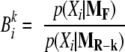10

By comparing the averaged likelihoods in the models with and without the interaction effects between the differential expression and the design factors, one can apply the same minimal threshold filter by Bayes factor. This leads to the selection of proteins whose differential expression is specific to certain cellular compartments or time points in the experiment.

Differential Expression with Time Course and Subcellular Localization Factors—

To demonstrate the use of the proposed methodology in the presence of experimental design factors, it was applied to the mouse data generated for the aforementioned PLN R9C mutant model. To identify proteins over- or underexpressed to varying degrees over time in different organelles, the full model and three reduced models have been fitted with the time factors nested within each organelle as seen in Equations 11–14,

11

12

13

14

where P_j and C_j are indicators for organelle and time course. Then the Bayes factors comparing M_F against the reduced models M_{R-(Cyto-Time)}, M_{R-(Micro-Time)}, and M_{R-(Mito-Time)} effectively test the significance of differential expression specific to time course effects within each organelle (cytosol, microsome, and mitochondria), respectively.

Applying the same criterion of Bayes factor greater than or equal to 10, which gives an approximate FDR of 5% according to the mixture model-based assessment, 444 differentially regulated proteins between mutant and wild type mice in specific time points within any of the three organelles were identified. Subsets of the 444 proteins pertaining to a particular change in expression (up/down-regulation), time point (8, 16, and 24 weeks), and organelle (cytosol, microsome, and mitochondria) were subjected to the functional annotation tool DAVID. Fig. 5A shows the clusters of proteins that were up- and down-regulated in the mutants at specific time points in each organelle. Fig. 5B shows a heat map of differential expression between each pair of mutant and wild type. In this figure, overexpression in PLN R9C mutant is highlighted in yellow, and underexpression is highlighted in blue.

Fig. 5.

Selected proteins and functional annotation in the mouse mutant model data set. A, clustered time course graphs by time points and organelles. Time points (T1, T2, and T3) correspond to week 8, 16, and 24, respectively. B, heat map of differential expression in the nine categories by time point and organelle. Yellow indicates overexpression in the PLN R9C mutant relative to the wild type, and blue indicates underexpression. Gene ontology terms with FDR-adjusted p value less than 0.05 are reported. dw, down; w, weeks.

Overall mitochondrial proteins concerned with muscle development and calcium ion binding showed the most drastic changes with up- and down-regulation in the earlier two time points (8 and 16 weeks). A good number of proteins involved with antioxidant activity and fatty acid metabolism were underexpressed in week 8 consistent with biological interpretation in the original study (29). At the organelle level, cytoskeleton organization- and actin cytoskeleton-related proteins were consistently overexpressed across all time points in cytosol. A cluster composed of endoplasmic reticulum targeting sequence, response to protein stimulus, and protein unfolding protein was highlighted in the up-regulated protein list in mitochondria at week 8. Many of the proteins in this list also appeared in the up-regulated list at week 16 with functions such as muscle protein, contractile fiber, muscle contraction, actin filament depolymerization, and negative regulation of cell organization. These same functions remained significant at week 24 in mitochondria. In the microsome, glucose metabolism was enriched in the down-regulated protein list consistent with antioxidant activities. Oxidative phosphorylation and ion transporter activity remained enriched across the time points in the up-regulated list in this organelle as well as in others. In summary, up-regulated calcium ion binding, cytoskeleton organization, and response to intracellular stress seem to have a strong association with the functional impairment on the cardiac ventricular muscle (see supplemental Table 4 for the selected proteins and their functional annotations).

DISCUSSION AND FUTURE WORK

At present, many studies that utilize spectral counting for relative quantification still rely on simple data analysis methods such as filtering based on -fold change ratios. Such an approach selects proteins based solely on the effect size without incorporating the variability. Therefore it may introduce a number of false positive calls in low abundance proteins where a small difference may result in artificially large -fold change ratios. More recently, a method has been described that improves the conventional signal-to-noise ratio statistics by adjusting the variance terms based on the analysis of the spectral counts across multiple replicates (27). The limiting factor of this method is that it requires a sufficient number of replicates. Because the variability is estimated separately for each protein, the estimates are likely to be coarse when the source of the variance calculation is merely a few data points. Moreover the limited number of or total absence of replicates makes it difficult to find a robust method to assign significance to these statistics and reasonably control global false discovery rates. For example, in the popular method of referencing observed statistics to the permutation distribution, the number of possible permutations is 70 at most when there are four replicates in each comparison group, which gives a low resolution permutation distribution vulnerable to outlying observations.

The method presented here has several advantages. It can be applied to a variety of situations including the comparative experiments that feature no or a few numbers of replicates within each biological condition. In contrast to other methods, by assuming the equal mean and variance relationship, the Poisson model of QSpec faces no issues with the absence of replicates. Because the protein-specific parameters are modeled as random numbers from a common population distribution, the method effectively pools statistical information needed for robust estimation (24) and provides a simple way to filter proteins based on a well established quantity known as Bayes factor (32) with an option of model-based FDR control.

The method can also be extended to more complex experimental designs where proteins are first separated into many fractions. In this instance, one can insert protein fraction-specific parameters in the model to account for the initial separation. In any case, hierarchical Bayes estimation will effectively pool the statistical information across the proteins from different fractions for more robust parameter estimations and attempt to overcome the paucity of information because of the small sample sizes. Another advantage of the method is the flexibility for possible extensions to more complicated data structures. It was demonstrated in this work that the Poisson model can easily incorporate design factors in analysis of variance form, including time course and subcellular localization factors. This class of GLMMs with hierarchical Bayes estimation can be applied to even more general data analysis scenarios. These include longitudinal profiling study without comparative design (no differential expression), replicate analysis where the reproducibility of quantitation is studied by comparing the within and between replicate variability, and protein-protein interaction study with a large number of pulldown experiments where the strength of interaction between pairs of proteins is validated based on the number of spectra corresponding to the interaction partners.

Yet there remain a number of areas for improvements in this modeling strategy. One well known problem with Poisson models is the potential violation of the assumption of the equal mean-variance relationship also termed the overdispersion problem. In data sets with many replicates, for instance, the observed data can include heterogeneous counts across replicates even within the same biological condition. In that case, the Poisson model with conventional assumptions may not work as efficiently. Furthermore using this model aggregating counts over replicates in a data set will produce largely identical results as in the case of applying it to the same data set but with replicates represented in it as separate experiments. In effect, this observation shows the drawback of the plain Poisson model from a different angle in that the model does not make full use of the variability observed in the data efficiently. Several extensions of the model are now being investigated. In addition to using the overdispersed Poisson model, another possibility is to use alternative distributions such as negative binomial models replacing the Poisson model used here. The latter model has a natural connection to Bayesian modeling through mixture model specification.

The discussion in this work was limited to spectral counts that were defined as the number of MS/MS spectra identified for each protein. However, related metrics such as the number of unique peptides are likely to contain additional useful information. Future work should involve detailed analysis of these different protein abundance parameters and their relative performance in different applications. To this end, future efforts should focus on designing multivariate statistical approaches that can effectively combine different abundance metrics leading to improved statistical power of detecting differential proteins. Furthermore such work should examine the effects of various instrument control settings on the accuracy of spectrum counting-based quantification.

Finally the protein inference problem of shotgun proteomics should not be overlooked because it also affects quantification (38). Peptides whose sequence is present in multiple proteins often cannot be unambiguously assigned to a particular protein or protein group in the protein summary file. The spectral counts for peptides shared among multiple proteins or protein isoforms should be appropriately weighted when computing the spectral count for each protein in a method similar to apportioning the probability of a peptide among all its corresponding proteins via peptide-protein weights when computing protein probabilities in ProteinProphet (39). For example, for a peptide identified from n MS/MS spectra and shared between two distinguishable proteins, A and B, its contribution to the spectral count of protein A could be taken as n × N_A^d/(N_A^d + N_B^d) where N_A^d and N_B^d are the spectral counts of proteins A and B, respectively, determined based on distinct (non-shared) peptides only. Note that the analysis presented in this work utilized spectral counts as provided in the original publications. Although less of an issue with yeast, in the mouse data set apportioning spectral counts of shared peptides as described above should provide more accurate protein abundance measures and thus more accurate results of the protein function enrichment analysis.

CONCLUSION

A statistical framework was presented for the significance analysis of differential expression in label-free shotgun proteomics using spectral counts. The statistical methodology developed in this work is a proteome-wide model-based assessment of differential expression using GLMM equipped with a hierarchical Bayes estimation procedure that borrows statistical strengths across all proteins. Unlike the conventional methods using ad hoc data transformation, signal-to-noise ratio, and posthoc data-driven adjustments, the proposed method is more powerful in finding differentially expressed proteins and robust to the variation because of the limited number of biological replicates at individual protein levels. The model showed superior performance in terms of its sensitivity of detection over existing methods. The real data analysis examples also illustrated the important advantages of handling the challenges because of the limited number of replicates and providing flexibility of extension of the model to more complicated study designs. It is expected that the computational framework presented in this work will be useful in a wide range of applications in label-free shotgun proteomics.

REFERENCES

- 1.Domon, B., and Aebersold, R. ( 2006) Mass spectrometry and protein analysis. Science 312, 212–217 [DOI] [PubMed] [Google Scholar]
- 2.Nesvizhskii, A. I., Vitek, O., and Aebersold, R. ( 2007) Analysis and validation of proteomic data generated by tandem mass spectrometry. Nat. Methods 4, 787–797 [DOI] [PubMed] [Google Scholar]
- 3.Gygi, S. P., Rist, B., Gerber, S. A., Turecek, F. Gelb, M. H., and Aebersold, R. ( 1999) Quantitative analysis of complex protein mixtures using isotope-coded affinity tags. Nat. Biotechnol. 17, 994–999 [DOI] [PubMed] [Google Scholar]
- 4.Ong, S. E., Blagoev, B., Kratchmarova, I., Kristensen, D. B., Steen, H., Pandey, A., and Mann, M. ( 2002) Stable isotope labeling by amino acids in cell culture, SILAC, as a simple and accurate approach to expression proteomics. Mol. Cell. Proteomics 1, 376–386 [DOI] [PubMed] [Google Scholar]
- 5.Ross, P. L., Huang, Y. N., Marchese, J. N., Williamson, B., Parker, K., Hattan, S., Khainovski, N., Pillai, S., Dey, S., Daniels, S., Purkayastha, S., Juhasz, P., Martin, S., Bartlet-Jones, M., He, F., Jacobson, A., and Pappin, D. J. ( 2004) Multiplexed protein quantitation in Saccharomyces cerevisiae using amine-reactive isobaric tagging reagents. Mol. Cell. Proteomics 3, 1154–1169 [DOI] [PubMed] [Google Scholar]
- 6.Goshe, M. B., and Smith, R. D. ( 2003). Stable isotope-coded proteomic mass spectrometry. Curr. Opin. Biotechnol. 14, 101–109 [DOI] [PubMed] [Google Scholar]
- 7.Bantscheff, M., Schirle, M., Sweetman, G., Rick, J., and Kuster, B. ( 2007) Quantitative mass spectrometry in proteomics: a critical review. Anal. Bioanal. Chem. 389, 1017–1031 [DOI] [PubMed] [Google Scholar]
- 8.Qian, W. J., Jacobs, J. M., Liu, T., Camp, D. G., and Smith, R. D. ( 2006) Advances and challenges in liquid chromatography-mass spectrometry-based proteomics profiling for clinical applications. Mol. Cell. Proteomics 5, 1727–1744 [DOI] [PMC free article] [PubMed] [Google Scholar]
- 9.Li, X., Yi, E. C., Kemp, C. J., Zhang, H., and Aebersold, R. ( 2005) A software suite for the generation and comparison of peptide arrays from sets of data collected by liquid chromatography-mass spectrometry. Mol. Cell. Proteomics 4, 1328–1340 [DOI] [PubMed] [Google Scholar]
- 10.Jaffe, J. D., Mani, D. R., Leptos, K. C., Church, G. M., Gillette, M. A., and Carr, S. A. ( 2006) PEPPeR, a platform for experimental proteomic pattern recognition. Mol. Cell. Proteomics 5, 1927–1941 [DOI] [PMC free article] [PubMed] [Google Scholar]
- 11.Listgarten, J., and Emili, A. ( 2005) Statistical and computational methods for comparative proteomic profiling using liquid chromatography-tandem mass spectrometry. Mol. Cell. Proteomics 4, 419–434 [DOI] [PubMed] [Google Scholar]
- 12.Liu, H., Sadygov, R. G., and Yates, J. R., III ( 2004) A model for random sampling and estimation of relative protein abundance in shotgun proteomics. Anal. Chem. 76, 4193–4201 [DOI] [PubMed] [Google Scholar]
- 13.Blondeau, F., Ritter, B., Allaire, P. D., Wasiak, S., Girard, M., Hussain, N. K., Angers, A., Legendre-Guillemin, V., Roy, L., Boismenu, D., Kearney, R. E., Bell, A. W., Bergeron, J. J., and McPherson, P. S. ( 2004) Tandem MS analysis of brain clathrin-coated vesicles reveals their critical involvement in synaptic vesicle recycling. Proc. Natl. Acad. Sci. U. S. A. 101, 3833–3838 [DOI] [PMC free article] [PubMed] [Google Scholar]
- 14.McAfee, K. J., Duncan, D. T., Assink, M., and Link, A. J. ( 2006) Analyzing proteomes and protein function using graphical comparative analysis of tandem mass spectrometry results. Mol. Cell. Proteomics 5, 1497–1513 [DOI] [PubMed] [Google Scholar]
- 15.Old, W. M., Meyer-Arendt, K., Aveline-Wolf, L., Pierce, K. G., Mendoza, A., Sevinsky, J. R., Resing, K. A., and Ahn, N. G. ( 2005) Comparison of label-free methods for quantifying human proteins by shotgun proteomics. Mol. Cell. Proteomics 4, 1487–1502 [DOI] [PubMed] [Google Scholar]
- 16.Ishihama, Y., Oda, Y., Tabata, T., Sato, T., Nagasu, T., Rappsilber, J., and Mann, M. ( 2005) Exponentially modified protein abundance index for estimation of absolute protein amount in proteomics by the number of sequenced peptides per protein. Mol. Cell. Proteomics 4, 1265–1272 [DOI] [PubMed] [Google Scholar]
- 17.Colinge, J., Chiappe, D., Lagache, S., Moniatte, M., and Bougueleret, L. ( 2005) Differential proteomics via probabilistic peptide identification scores. Anal. Chem. 77, 596–606 [DOI] [PubMed] [Google Scholar]
- 18.Zybailov, B., Mosley, A. I., Sardiu, M. E., Coleman, M. K., Florens, L., and Washburn, M. P. ( 2006) Statistical analysis of membrane proteome expression changes in Saccharomyces cerevisiae. J. Proteome Res. 5, 2339–2347 [DOI] [PubMed] [Google Scholar]
- 19.Lu, P., Vogel, C., Wang, R., Yao, X., and Marcotte, E. M. ( 2007) Absolute protein expression profiling estimates the relative contributions of transcriptional and translational regulation. Nat. Biotechnol. 25, 117–124 [DOI] [PubMed] [Google Scholar]
- 20.Fu, X., Gharib, S. A., Green, P. S., Aitken, M. L., Frazer, D. A., Park, D. R., Vaisar, T., and Heinecke, J. W. ( 2008) Spectral index for assessment of differential protein expression in shotgun proteomics. J. Proteome Res. 7, 845–854 [DOI] [PubMed] [Google Scholar]
- 21.Zhang, B., VerBerkmoes, N. C., Langston, M. A., Uberbacher, E., Hettich, R. I., and Samatova, N. F. ( 2006) Detecting differential and correlated protein expression in label-free shotgun proteomics. J. Proteome Res. 5, 2909–2918 [DOI] [PubMed] [Google Scholar]
- 22.Xia, Q., Wang, T., Park, Y., Lamont, R. J., and Hackett, M. ( 2007) Differential quantitative proteomics of Porphyromonas gingivalis by linear ion trap mass spectrometry: non-label methods comparison, q-values and LOWESS curve fitting. Int. J. Mass Spectrom. 259, 105–116 [DOI] [PMC free article] [PubMed] [Google Scholar]
- 23.Tusher, V. G., Tibshriani, R., and Chu, G. ( 2001) Significance analysis of microarrays applied to the ionizing radiation response. Proc. Natl. Acad. Sci. U. S. A. 98, 5116–5121 [DOI] [PMC free article] [PubMed] [Google Scholar]
- 24.Parmigiani, G., Garrett, E. S., Irizarry, R. A., and Zeger, S. L. ( 2003) The Analysis of Gene Expression Data, Springer-Verlag, New York
- 25.Do, K. A., Muller, P., and Vannucci, M. ( 2006) Bayesian Inference for Gene Expression and Proteomics, Cambridge University Press, New York
- 26.Segal, E., Friedman, N., Kaminski, N., Regev, A., and Koller, D. ( 2005) From signatures to models: understanding cancer using microarrays. Nat. Genet. 37, S38–S45 [DOI] [PubMed] [Google Scholar]
- 27.Pavelka, N. M., Fournier, M. L., Swanson, S. K., Pelizzola, M., Ricciardi-Castagnoli, P., Florens, L., and Washburn, M. P. ( 2008) Statistical similarities between transcriptomics and quantitative shotgun proteomics data. Mol. Cell. Proteomics 7, 631–644 [DOI] [PubMed] [Google Scholar]
- 28.Zeger, S. L., and Karim, M. R. ( 1991) Generalized linear models with random effects; a Gibbs sampling approach. J. Am. Stat. Assoc. 86, 79–86 [Google Scholar]
- 29.Gramolini, A. O., Kislinger, T., Alikhani-Koopaei, R., Fong, V., Thompson, N. J., Isserlin, R., Sharma, P., Oudit, G. Y., Tivieri, M. G., Fagan, A., Kanna, A., Higgins, D., Huedig, H., Hess, G., Arab, S., Seidman, J. G., Seidman, C. E., Frey, B., Perry, M., Backx, P. H., Liu, P. P., MacLennan, D. H., and Emili, A. ( 2008) Comparative proteomic profiling of a phospholamban mutant mouse model of dilated cardiomyopathy reveals progressive intracellular stress responses. Mol. Cell. Proteomics 7, 519–533 [DOI] [PubMed] [Google Scholar]
- 30.Al-Shahrour, F., Minguez, P., Tarraga, J., Montaner, D., Alloza, E., Vazquerizas, J. M. M., Conde, L., Blaschke, C., Vera, J., and Dopazo, J. ( 2006) BABELOMICS: a systems biology perspective in the functional annotation of genome-scale experiments. Nucleic Acids Res. 34, W472–W476 [DOI] [PMC free article] [PubMed] [Google Scholar]
- 31.Dennis, G., Jr., Sherman, B. T., Hosack, D. A., Yang, J., Gao, W., Lane, H. C., and Lempicki, R. A. ( 2003) DAVID: database for annotation, visualization, and integrated discovery. Genome Biol. 4, P3. [PubMed] [Google Scholar]
- 32.Jeffreys, H. ( 1961) The Theory of Probability, Oxford University Press, Oxford
- 33.Efron, B. ( 2004) Large-scale simultaneous hypothesis testing: the choice of a null hypothesis. J. Amer. Stat. Assoc. 99, 96–104 [Google Scholar]
- 34.Efron, B. ( 2007) Size, power and false discovery rates. Ann. Stat. 35, 1351–1377 [Google Scholar]
- 35.Cai, L., Huang, H., Blackshaw, S., Liu, J. S., Cepko, C., and Wong, W. H. ( 2004) Clustering analysis of SAGE data using a Poisson approach. Genome Biol. 5, R51. [DOI] [PMC free article] [PubMed] [Google Scholar]
- 36.Smyth, G. K. ( 2004) Linear models and empirical Bayes methods for assessing differential expression in microarray experiments. Stat. Appl. Genet. Mol. Biol. 3, Article 3 [DOI] [PubMed]
- 37.Robert, C. P., and Casella, G. ( 2004) Monte Carlo Statistical Methods, Springer, New York
- 38.Nesvizhskii, A. I., and Aebersold, R. ( 2005) Interpretation of shotgun proteomic data. Mol. Cell. Proteomics 4, 1419–1440 [DOI] [PubMed] [Google Scholar]
- 39.Nesvizhskii, A. I., Keller, A., Kolker, E., and Aebersold, R. ( 2003) A statistical model for identifying proteins by tandem mass spectrometry. Anal. Chem. 75, 4646–4658 [DOI] [PubMed] [Google Scholar]
Associated Data
This section collects any data citations, data availability statements, or supplementary materials included in this article.