A general computational method for robustness analysis with applications to synthetic gene networks

Abstract

Motivation: Robustness is the capacity of a system to maintain a function in the face of perturbations. It is essential for the correct functioning of natural and engineered biological systems. Robustness is generally defined in an ad hoc, problem-dependent manner, thus hampering the fruitful development of a theory of biological robustness, recently advocated by Kitano.

Results: In this article, we propose a general definition of robustness that applies to any biological function expressible in temporal logic LTL (linear temporal logic), and to broad model classes and perturbation types. Moreover, we propose a computational approach and an implementation in BIOCHAM 2.8 for the automated estimation of the robustness of a given behavior with respect to a given set of perturbations. The applicability and biological relevance of our approach is demonstrated by testing and improving the robustness of the timed behavior of a synthetic transcriptional cascade that could be used as a biological timer for synthetic biology applications.

Availability: Version 2.8 of BIOCHAM and the transcriptional cascade model are available at http://contraintes.inria.fr/BIOCHAM/

Contact: gregory.batt@inria.fr

1 INTRODUCTION

Robustness can be defined as the capacity of a system to maintain a function in the face of perturbations. Over the years, many studies have demonstrated theoretically and experimentally that robustness is a key property of numerous biological processes, and have proposed mechanisms that promote robustness (e.g. Barkai and Leibler, 1997; Batt et al., 2007; Chaves et al., 2007; Ciliberti et al., 2007; Davidson and Levine, 2008; El-Samad et al., 2005; Gonze et al., 2002; Ingolia, 2004; Shen et al., 2008; Shinar et al., 2007; Stelling et al., 2004b; von Dassow et al., 2000). Robustness is now regarded as one of the fundamental characteristics of biological systems because it allows their correct functioning in presence of molecular noise and environmental fluctuations. Excellent reviews have surveyed the role of biological robustness, and discussed its interesting relations with evolvability of biological systems, modularity of biological networks and the trade-off between robustness and fragility (e.g. Kitano, 2004; Stelling et al., 2004a; Yi et al., 2000). In particular, in the context of synthetic biology, these are key issues to take into account at the design level.

Intuitively, the notion of robustness seems easy to define. One considers (i) a particular system, (ii) a particular function and (iii) a particular set of perturbations, and one assesses how perturbations affect (or not) the given function. However, with the notable exception of Kitano (2007), no general formal definition of robustness has been proposed. The precise definition of robustness is generally highly problem-specific. This makes it difficult to discuss and compare the robustness found in different contexts, or even in similar contexts but computed using different formal definitions of robustness. In Kitano (2007), the mathematical foundations of a theory of biological robustness is proposed, with the aim of providing a unified perspective on robustness.

Although very interesting from a theoretical point of view, Kitano's definition might be too general when applying it to particular problems. Indeed the definition relies on a so-called evaluation function, defined using an unspecified, problem-dependent real-valued performance function. Here, we propose to define the evaluation function using the newly introduced notion of violation degree of temporal logic formulae (Fages and Rizk, 2008). Intuitively, the violation degree reflects the distance between a particular behavior of the perturbed system, given as a numerical timed trace, and the expected reference behavior, expressed by a temporal logic formula. Because (i) temporal logics are expressive languages to formalize temporal behavior of dynamical systems and (ii) the violation degree can be automatically computed, our instantiation of Kitano's definition is both general and computational. The main contribution of our work is that we propose a computational approach for—and an implementation of—the automatic estimation of the robustness that applies to a broad class of dynamical properties and a large variety of possible perturbations. We simply require that the property describing the expected behavior can be expressed in temporal logic and that the behavior of the system can be represented by a numerical trace (possibly obtained by numerical simulation of deterministic or stochastic models).

A second contribution of this work is that we propose two closely related but different notions of robustness that have been used indiscriminately in publications, namely the absolute robustness of a system, representing the average functionality of the system under perturbations, and the relative robustness with respect to a given nominal behavior of the system, quantifying the impact of perturbations on the nominal behavior. We believe that distinguishing these two notions will help to clarify the analysis of robustness of biological systems. Undoubtedly, formal definitions are useful for making this distinction.

The applicability and biological relevance of our approach is illustrated on the analysis of the robustness of the timed response of a synthetic transcriptional cascade built in Escherichia coli. This system presents a high cell-to-cell variability that prevents using it as a biological timer. We look for parameter modifications that improve the robustness of a ‘well-timed’ behavior.

The remainder of this article is organized as follows. In the next section, we provide a brief description of the violation degree notion introduced in Fages and Rizk (2008). In Section 3, we present the proposed method for robustness estimation and its implementation in BIOCHAM 2.8. In Section 4, we detail the application of our method to the analysis of the robustness of the synthetic transcriptional cascade.

2 VIOLATION DEGREE OF TEMPORAL LOGIC PROPERTIES

We first define the Boolean semantics of linear temporal logic (LTL) on timed numerical traces (Section 2.1). Then, we show how using the variable abstraction technique of Section 2.2, we can define a continuous satisfaction degree for temporal logic formulae (Section 2.3) better adapted to a quantitative notion of robustness.

2.1 Temporal logic semantics of numerical traces

In this article, we consider that the behavior of a biological system is described by numerical timed traces. These traces can be obtained either by experimentation on the actual system or by numerical simulation of stochastic or deterministic models. Formally, a numerical trace is a finite sequence of tuples describing system's evolution with time: T=(s₀, s₁,…, s_n), with 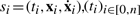being a strictly increasing sequence of time points, and being vectors of state variable values and of their derivatives at time t_i. In Figure 1a, a hypothetical evolution of a protein concentration is represented. The associated trace is T=((0, 6, 1.3), (2, 8, 0.8),…, (24, 5, 0)).

Fig. 1.

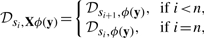
(a) Numerical trace depicting the time evolution of a protein concentration. (b) Satisfaction domain 𝒟_T,ϕ(y) of QFLTL formula ϕ(y)=F([A]>y₁ ∧ F[A]<y₂) and trace T, and LTL formulae ϕ₁, ϕ₂ and ϕ₃, represented in formula space. (c and d) Representation of satisfaction domains for three perturbations p₁, p₂, and p₃. 𝒟_pi denotes 𝒟_{Tpi, ϕ(y)}. In (c), the intersection of satisfaction domains (shaded) is not empty and Rsd^s_ϕ,P=3. The property is satisfied for all perturbations. In (d), the intersection of satisfaction domains is empty and Rsd^s_ϕ,P=∞.

We use LTL to express dynamical properties of biological systems. Temporal logics have been developed to specify the behavior of (usually discrete) dynamical systems (Emerson, 1990). Typical properties include reachability (the system can reach a given state), inevitability (the system will necessarily reach a given state), invariance (a property is always true), response (an event necessarily triggers a specific behavior) and infinite occurrences of events (such as oscillations). Illustrative examples of the expressiveness of temporal logics in systems biology can be found in Antoniotti et al. (2003); Batt et al. (2005); Bernot et al. 2004); Calzone et al. (2006) and Chabrier and Fages (2003). LTL formulae are built using atomic propositions and LTL operators.

In our approach, atomic propositions π express real-valued linear constraints on time, protein concentrations and their derivatives. The infinite set of atomic propositions is denoted by Π.

LTL operators include the usual logical operators, such as negation (¬), logical and (∧), logical or (ν) and implication (→), and specific temporal operators, such as next (X), future (F), globally (G) and until (U). X ϕ, F ϕ, G ϕ and ϕ U ψ, respectively, mean that a property ϕ holds at the next time, at some future time, holds for all future times or holds continuously until another property ψ holds. These operators can be combined to express complex dynamical properties. For example, the trace T represented in Figure 1a satisfies the formula ϕ₁=F([A]>7 ∧ F [A]<3), expressing that at some time point, protein A concentration exceeds 7 and later goes below 3. Because negations can be pushed to atomic propositions with the usual duality properties of operators, and the set of atomic propositions is closed by negation, we consider without loss of generality only negation-free LTL formulae.

The standard semantics of LTL formulae is generally defined with respect to infinite executions, i.e. infinite traces. Because in our case, the traces are finite, the usual semantics of LTL has to be adapted. Let T=(s₀, s₁,…, s_n) be a finite numerical trace, π∈Π be an atomic proposition and ϕ, ψ be LTL formulae. Then the semantics of LTL formulae with respect to finite traces is defined inductively as T ⊧ ϕ iff s₀ ⊧ ϕ, and

• s_i ⊧ π iff satisfies π with the usual semantics,

• s_i ⊧ ϕ ∧ ψ iff s_i ⊧ ϕ and s_i ⊧ ψ,

• s_i ⊧ ϕ ν ψ iff s_i ⊧ ϕ or s_i ⊧ ψ,

• s_i ⊧ Xϕ iff i<n and s_i+1 ⊧ ϕ, or i=n and s_n ⊧ ϕ,

• s_i ⊧ Fϕ iff ∃ j∈[i, n] such that s_j ⊧ ϕ,

• s_i ⊧ Gϕ iff ∀ j∈[i, n], s_j ⊧ ϕ,

• s_i ⊧ ϕUψ iff ∃ j∈[i, n] s. t. s_j ⊧ ψ and ∀ k∈[i, j−1], s_k ⊧ ϕ.

Our semantics of LTL coincides with the standard semantics used on finite traces completed by a self-loop on the last state (Fages and Rizk, 2008). This semantics differs from the neutral semantics of Eisner et al. (2003) for finite traces only for the next operator, which in their definition is always false on the last state, whereas in our case it enjoys the duality property ¬Xϕ=X¬ϕ and either Xϕ or X¬ϕ holds. In practice, the next operator being mainly used to detect local extrema, this difference of interpretation is not significant.

It is worth noticing that when the numerical trace corresponds to a discrete representation of a continuous process, the discrete time semantics that we use may cause that particular events are ‘missed’ independently of the numerical errors that can be made by the numerical integration method. For example, the formula F([A]≥10) interpreted on trace T of Figure 1a and expressing that eventually [A] exceeds 10 might be found true or false depending on the integration step and precision. So care must be taken when checking temporal properties on finite discrete time traces [for a discussion, see Eisner et al. (2003); Fainekos and Pappas (2007) and Maler et al. (2008), and references therein].

2.2 From model checking to constraint solving

The Boolean interpretation of temporal logic is not well adapted to defining a quantitative notion of robustness. Indeed, neither of the two formulae ϕ₂=F([A]>12 ∧ F [A]<3) and ϕ₃=F([A]>14 ∧ F [A]<3) hold for the trace T of Figure 1a. However, intuitively ϕ₂ is closer to satisfaction than ϕ₃, since it only requires that [A] reaches 12 instead of 14.

To provide a formal definition of a continuous degree of satisfaction of LTL formulae, we first consider quantifier-free LTL (QFLTL) formulae with free (non-state) real-valued variables y (Fages and Rizk, 2008). Then, the original model checking problem is transformed into the following constraint solving problem: for which values y does ϕ(y) hold on T? Accordingly, we define for any trace T the satisfaction domain of ϕ(y) as the set of values y for which ϕ(y) holds:

(1)

In the sequel, ϕ(y) will denote the QFLTL formula obtained by variable abstraction from a (QF)LTL formula ϕ.

Interestingly, an LTL formula can be seen as an instance of a QFLTL formula obtained by abstracting the constants appearing in the formula by new variables y∈ℝ^q. For example, to ϕ₁=F([A]>7 ∧ F [A]<3), we associate the formula ϕ(y)=ϕ(y₁, y₂)=F([A]>y₁ ∧ F [A]<y₂). Then we have ϕ₁=ϕ(7, 3). Moreover, one can easily check that for our example trace T, 𝒟_T,ϕ(y1,y2)={y₁≤10 ∧ y₂≥2}, 10 and 2 being, respectively, the maximal and minimal values of [A] in T.

More generally, this variable abstraction/instantiation process allows us to view a LTL formula as a point in the QFLTL formula space ℝ^q, where q is the number of constants appearing in ϕ (or the number of constants that are replaced by variables, if not all constants are abstracted away). In Figure 1b, ϕ₁, ϕ₂, ϕ₃ and 𝒟_T,ϕ are represented in this formula space.

Given any trace T=(s₀, s₁,…, s_n) and formula ϕ(y) we showed in (Fages and Rizk, 2008) that the satisfaction domain 𝒟_T,ϕ(y) can be computed by induction on T and the subformulae of ϕ(y) using the equalities of Proposition 1.

Proposition 1 —

[Computation of satisfaction domains (Fages and Rizk, 2008)]

• 𝒟_T,ϕ(y)=𝒟_s0,ϕ(y),

• 𝒟_si,π(y)={y∈ℝ^q∣π(y) holds with the usual semantics},

• 𝒟_si,ϕ(y)∧ψ(y)=𝒟_si,ϕ(y)∩𝒟_si,ψ(y),

• 𝒟_si,ϕ(y)νψ(y)=𝒟_si,ϕ(y)∪𝒟_si,ψ(y),

• 

• 𝒟_si,Fϕ(y)=∪_j∈[i,n]𝒟_sj,ϕ(y),

• 𝒟_si,Gϕ(y)=∩_j∈[i,n]𝒟_sj,ϕ(y),

• 𝒟_{si,ϕ(y)Uψ(y)}=∪_j∈[i,n](𝒟_sj,ψ(y)∩∩_{k∈[i,j−1]}𝒟_sk,ϕ(y)).

The atomic propositions in ϕ(y) being linear constraints on free variables y, the satisfaction domains are finite unions and intersections of polytopes that can be computed with standard polyhedra libraries. Although generally efficient, these operations require in the worst case a time exponential in the formula space dimension. They are, however, independent on the number of state variables.

2.3 Violation degree

To quantify how far from satisfaction a system's behavior is, we introduce the violation degree vd(T, ϕ) of a formula ϕ with respect to trace T as the distance between the actual specification and validity domain 𝒟_T,ϕ(y) of the QFLTL formula ϕ(y) obtained by variable abstraction:

The violation degree has thus a simple interpretation, since it quantifies by how much a given LTL formula must be changed to hold on a given numerical trace.

Considering again our example in Figure 1b and using the Euclidean distance, we have that vd(T, ϕ₁)=0, meaning that the formula is satisfied by T, and vd(T, ϕ₂)=2 and vd(T, ϕ₃)=4, reflecting that T is further from satisfaction of ϕ₃ than of ϕ₂.

We would like to emphasize that abstracting constants by variables in temporal logic formulae is a means to define a metric on the set of formulae. All set operations and distance computations are made in the corresponding metric space, known as the formula space. It might seem more intuitive to define distances directly between traces. For example, Fainekos and Pappas (2006) use with a similar aim—defining a continuous interpretation of temporal logic formulae on traces—the distance between a given trace T and the set of traces satisfying a formula ϕ. One major advantage of our approach is that the dimensionality of the formula space (number of abstracted constants) is generally much lower than the dimensionality of the trace space (trace length). Performing set operations and distance computation in low-dimensional spaces may strongly affect the practical applicability of these methods. In Donaldson and Gilbert (2008) a similar notion of violation degree has been recently proposed, also based on the definition of a satisfaction domain of temporal logic formulae. However, the computation of the (finite) satisfaction domain is made by sampling the formula space rather than by constraint solving. In this article, we will use the Euclidean distance. However, many other distances can be used (e.g. Manhattan or Chebyshev), depending on the desired interpretation of distance and, as we will see in the next paragraph, on the desired interpretation of robustness.

To define the robustness of a behavior, it is more convenient to reason with a positive notion that describes how good the (possibly perturbed) system performs, i.e. satisfies a dynamical property. To do so, we introduce the notion of continuous satisfaction degree of a formula with respect to a trace T:

(2)

where vd is the violation degree previously introduced. The satisfaction degree is normalized such that it ranges between 0 and 1, with a satisfaction degree equal to 1 when the property is true and tending toward 0 when the system is far from satisfying the expected property. For some applications, the satisfaction degree might be normalized differently, using a given constant K instead of the ones in Equation (2).

3 ROBUSTNESS DEFINITIONS AND COMPUTATIONS

3.1 Absolute robustness

In this article, we mainly use Kitano's general definition of robustness. In Kitano (2007), the robustness of a property a of a system s with respect to a set of perturbations P is defined as the average of an evaluation function D_a^s of the system over all perturbations p∈P, weighted by the perturbation probabilities prob(p):

(3)

One should emphasize that this definition is very general and can be used in many cases. Unfortunately, Kitano does not provide much information on how to define the so-called evaluation function D_a^s of the system. This function should determine if the system still maintains its function under a perturbation and to what degree. The evaluation function needs to be defined for each specific problem in an ad hoc manner and re-implemented for the computation of the robustness. A central contribution of this article is to demonstrate that using the notion of satisfaction degree presented previously, one can provide a general computational framework based on temporal logic and Kitano's definition that can be used to evaluate the robustness of broad types of dynamical properties and perturbations.

Formally, the robustness of the system is defined as:

(4)

where ϕ is the specification of the functionality in temporal logic and T_p is the trace representing the behavior of the system under perturbation p. This notion of robustness corresponds to a mean functionality, that is, describes on average how the system behaves under perturbations. To illustrate this, consider the plots 1 and 2 of Figure 2 that describe the performance D_a^s—or equivalently in our case, the satisfaction degree—of two hypothetical systems in the face of perturbations p. Because these two plots have the same average, the robustness of these two systems would be equal for evenly distributed perturbations. For example, in a bioengineering context, if the ‘property’ reflects the quantity of some product exported by cells, these two systems will indeed produce on average the same quantity of the desired product.

Fig. 2.

Systems having same absolute robustness (1 and 2) or same relative robustness (1 and 3), assuming evenly distributed perturbations. Performance functions of Systems 1 and 2 have same the average, whereas the performance function of System 3 is half of the one of System 1.

This notion of robustness has been used in Ingolia (2004), Ma et al. (2006) and von Dassow et al. (2000) to study the influence of large parameter variations on the Drosophila segment polarity pattern formation. Ma et al. (2006) used a Boolean criteria requiring a ‘pattern penality function’ pen(x(t)) to be below a given threshold θ^*=0.0125 at 600 and 800 min. The QFLTL formula ϕ(θ)=G(time∈[600, 800]→pen(x(t))≤θ) states that the penalty function must be below θ in the entire time interval, and the satisfaction degree of a system's behavior T_p and ϕ(θ^*) provides a quantitative measure of the distance between T_p and the reference behavior.

3.2 Relative robustness

When comparing plots 1 and 2 of Figure 2, it appears that the consequences of perturbations of the nominal behavior are not the same, with T₀ the nominal behavior. In System 1, perturbations degrade the system's performance more severely than in System 2. So, with a different meaning of robustness, one could say that System 2 is more robust than System 1. These two robustness interpretations (as average behavior or as impact of perturbations on nominal behavior) have been indiscriminately used in the literature (see e.g. Davidson et al., 2003; von Dassow et al., 2000). To reflect this second interpretation, let us define the relative robustness of a system with respect to a nominal behavior as the system's robustness divided by its nominal performance, that is, by the satisfaction degree of the reference behavior.

(5)

where T_p^* denotes the unperturbed, nominal behavior of the system. In Figure 2, one can distinguish the relative robustness of Systems 1 and 2 with respect to their nominal performance, reflecting that the performance is more impacted by perturbations in System 1 than in System 2. The performance function of System 3 equals half of the performance function of System 1. Consequently, these systems have the same relative robustness with respect to their nominal performance, although they have different absolute robustness.

Gonze et al. (2002) studied the influence of low molecule numbers on circadian oscillation periods. Stochastic simulation results are compared with the behavior of a corresponding deterministic model. The period is defined as the time interval separating two successive upward crossings of the mean value of protein or mRNA concentrations. One can study such oscillations with our approach using, for example, the QFLTL formula F(x<m∧X(x>m)∧time=t₁∧F(x<m∧X(x>m)∧time=t₂))∧t₂−t₁<b, expressing that the maximal time between two successive upwards crossing events is less than b, with m the mean value of x, that needs to be computed beforehand. More complex temporal behaviors, such as the existence of 13 mitotic cycles followed by G2 arrest (Calzone et al., 2007), could be expressed similarly and subsequently analyzed using our approach.

3.3 Robust satisfaction degree

Using the notion of satisfaction domain, we can also define the distance from robust satisfaction of a property ϕ with respect to a set of perturbations P as dist(∩_p𝒟_Tp, ϕ). This distance reflects the minimal change in the formula such that it holds for all perturbations. Then, we define the robust satisfaction degree as:

(6)

This notion allows us to distinguish whether it is possible to relax the specification to have it satisfied for all perturbations or not. In the case of Figure 1c, one can guarantee that the system always presents a (possibly suboptimal) behavior. Moreover, the closest property robustly satisfied (i.e. such that can provide interesting hints for the system's design: because , it suggests that only the first value in ϕ (i.e. the maximum of [A] in T) needs to be modified.

In Batt et al. (2007), an approach is presented to check that a (model of a) synthetic transcriptional cascade satisfies a given input/output steady state property for sets of parameters. More precisely, it was required for all parameters in a given set, that if the inducer concentration is low (u_aTc<100), then at steady state the fluorescence is low (x_eyfp<500), and if the inducer concentration is high (u_aTc>400), then so is the steady state fluorescence (x_eyfp>500000). When considering the QFLTL formula ϕ(m, M)=u_aTc<100→FG(x_eyfp<m)∧u_aTc>400→FG(x_eyfp>M), it is additionally possible to find the set of properties satisfied by all parameters. This can be done by computing the intersection of all satisfaction domains ∩_p𝒟_Tp,ϕ. The robust satisfaction degree of the property ϕ(m, M) provides an indication of how close to robust satisfaction our requirement is.

3.4 Implementation

For the computation of R^s_ϕ,P, R^s,p*_ϕ,P and Rsd^s_ϕ,P, one needs to distinguish whether the set of perturbations is finite (e.g. gene knockouts) or infinite (e.g. normally distributed parameter variations). In the first case, the values can be computed exactly, whereas in the second case, they can be estimated by sampling the perturbation set for sufficiently many perturbations.

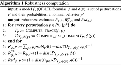
The following algorithm is implemented in version 2.8 of the freely available tool BIOCHAM, a modeling environment for the analysis of biological systems (Calzone et al., 2006). Given an ODE model f, a set P of perturbations of initial conditions or parameters, and (QF)LTL properties ϕ and ϕ(y), the tool computes the robustness, the relative robustness and the robust satisfaction degree of the property with respect to the given perturbations. The computation of the trace T_p is done by numerical integration. The computation of the satisfaction domain 𝒟_Tp,ϕ(y) is made by induction on the formula structure, using for each subformula a direct implementation of the definition. Polytopes operations are implemented in BIOCHAM using a standard polyhedral library (Bagnara et al., 2008).

4 APPLICATION TO ROBUSTNESS ANALYSIS OF A TRANSCRIPTIONAL CASCADE

We consider the design of a synthetic transcriptional cascade that could be used for the temporal sequencing of events in synthetic biology applications. This cascade has been build by Hooshangi and colleagues (2005) and here we investigate the robustness of a desired behavior, and the possibilities to make it more robust. To do so, after having introduced the system, we formalize the expected behavior, develop a model of the system taking into account the observed variability and apply the method presented previously to investigate the robustness of the desired property.

4.1 System description

We consider a cascade of transcriptional inhibitions built in E. coli (Hooshangi et al., 2005). The network is represented in Figure 3a. It is made of four genes: tetR, lacI, cI and eyfp that code, respectively, for three repressor proteins, TetR, LacI and CI, and the fluorescent protein EYFP. The fluorescence of the system, due to the protein EYFP, is the measured output. The system can be controlled by the addition or removal of a small diffusible molecule, aTc, in the growth media. More precisely, aTc binds to TetR and relieves the repression of lacI. The aTc concentration thus serves as a controllable input to the system. It is intuitively clear that the output (i.e. the fluorescence) of the system at steady state will be low for low inputs (i.e. aTc concentration), and high for high inputs. Moreover, it has been shown that the time response of the system to an inducer addition is characterized by a rapid increase of the fluorescence, preceded by a significant lag phase. Unfortunately, a high cell-to-cell variability has also been observed. The heterogeneity of the cell responses makes it difficult to use this system as a biological timer, for example for developmental programs as suggested in Hooshangi et al. (2005). In this context, as for many synthetic biology applications, having even a low proportion of cells sending a signal too early or too long might compromise the correct functioning of the whole system. Our goal here is to precisely investigate the possibilities to obtain a robustly ‘well-timed’ system, that is to ensure that all cells will indeed change state in a given time window.

Fig. 3.

Synthetic transcriptional cascade. (a) TetR represses lacI, LacI represses cI and CI represses eyfp. aTc controls the repression of lacI by TetR. The fluorescence of the protein EYFP is the output. (b) Graphical representation of a ‘well-timed’ behavior: fluorescence remains below 10³ until time t₁, exceeds 10⁵ after time t₂ and switches between low and high levels in Δ_t time. One expects that t₁>150, t₂<450 and Δ_t<150. Crosses represent experimental data from Hooshangi et al. (2005).

4.2 Specifying the expected behavior

Here, we consider that the system is well-timed if the fluorescence remains below 10³ for at least 150 min, then exceeds 10⁵ after at most 450 min, and switches rapidly from low to high levels, that is, in less than 150 min. These specifications are consistent with the experimentally observed behavior of the cell population. These specifications are graphically represented in Figure 3b and can be formalized in temporal logic as follows:

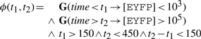which is abstracted into

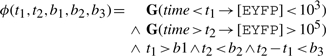for the computation of validity domains and satisfaction degree in a given trace.

4.3 Modeling the system's variability

There are many ways to model cell variability (see for example Manninen et al., 2006). Our goal here is to construct a simple model such that the predicted behavior and standard deviation are in agreement with the available experimental data. We first develop a simple ODE model similar to Batt et al. (2007) but using Hill functions, with parameters fitted to experimental data (Figures 4a and B). These parameter reference values are denoted by p^* in the sequel. Second, we consider various ways to model cell variability, including stochastic differential equations with either additive or multiplicative noise and random parameter variations with (log)normal distributions. We have obtained a good qualitative and quantitative agreement between the predicted and observed mean and standard deviation for log-normally distributed parameters, as shown in Figure 5a and b. So we selected these log-normal parameter distributions as our ‘perturbation model’. Using either stochastic differential equations or normally distributed parameters, we have not been able to find an agreement between model predictions and experimental observations (data not shown). This could be partially explained by the very high cell-to-cell variability. In particular, the observed coefficient of variation reaches 1.4 at some time point, meaning that the standard deviation is higher than the mean.

Fig. 4.

(a) ODE model of the transcriptional cascade. The concentrations of protein LacI, CI, EYFP and of aTc are denoted by x_lacI, x_cI, x_eyfp and u_aTc, respectively. The concentration of the constitutively expressed protein TetR is assumed constant. (b) Reference parameter values p^* and (c) parameter distributions modeling system's variability. σ is a noise intensity parameter vector.

Fig. 5.

(a) Temporal evolution of the fluorescence following addition of aTc. Crosses, dotted line and solid line represent experimental data from Hooshangi et al. (2005), predictions obtained using the ODE model with reference parameters p^*, and average of 5000 numerical simulations of the ODE model with log-normally distributed parameters, respectively. (b) Temporal evolution of the coefficient of variation of the fluorescence following addition of aTc. Crosses and solid line represent coefficient of variations obtained from experimental data in Hooshangi et al. (2005) and from 5000 numerical simulations of the ODE model with log-normally distributed parameters with mean p^*, respectively. (c) Numerical simulations of the ODE model with log-normally distributed parameters with mean p^*. (d) Distribution of satisfaction degrees for 5000 numerical traces of the perturbed transcriptional cascade model. The corresponding robustness is .

4.4 Improving robustness of the desired behavior

Having specified the ‘well-timed’ behavior and found an ODE model and a perturbation model, we wondered whether the system is robustly well-timed, and to what degree. When considering 5000 log-normally distributed parameter values in the 16 D parameter space, we estimated the robustness of the system as : the specification is not robustly satisfied. As expected, the property holds for the reference parameter values p^* (i.e. sd(T_p^*, ϕ)=1), and consequently the robustness and absolute robustness are equal (). The distribution of the satisfaction degree is represented in Figure 5d, showing that although the majority of timed traces satisfies the specification, this is not always the case. On average, each numerical simulation lasts 150 ms, and each satisfaction degree computation lasts 50 ms (∼500 time points/trace; Dual Core, 2 GHz, 2 GB RAM). For this application and in all our computations, the limiting factor is numerical simulation.

As said earlier, for most synthetic biology applications, a more robust timer would be needed. Can we find other parameters so as to improve the robustness of the system with respect to similar parameter perturbations? To do so, we use the state-of the-art non-linear optimization tool CMAES that uses a covariance matrix adaptation evolution strategy Hansen and Ostermeier (2001), with the robustness as optimization criteria (i.e. as fitness function). We found the following parameter values: 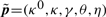, with

The comparison between original parameters p^* and so-called optimized parameters reveals that the EYFP production rate and the Hill coefficients η have been significantly increased. Given that one wants to ensure a fast transition between the low and high states, these parameters were obvious targets for optimizations. Because tuning Hill coefficients is experimentally difficult, we looked for and found parameters with unchanged Hill coefficients that ensure a robust well-timed behavior.

Numerical integrations illustrate that the expected behavior is indeed more robustly obtained (compare Figures 5c and 6a). Interestingly, the coefficient of variation suggests that cell-to-cell variability will be significantly decreased when the time constraints hold (for time<150) and is significantly increased otherwise (for 150<time<450, see Figure 6b). It would be interesting to study whether this feature appears systematically for parameter variations improving the robustness of the desired behavior. This could reveal trade-offs between robustness and fragility (Kitano, 2004).

Fig. 6.

Numerical simulations of the ODE model with 5000 log-normally distributed parameters with mean . (a) Temporal evolution of the fluorescence following addition of aTc. (b) Temporal evolution of the coefficient of variation of the fluorescence. Crosses and solid line represent coefficient of variations obtained from experimental data in Hooshangi et al. (2005) and from numerical simulations, respectively.

4.5 Parameter influence on robust behavior

To obtain a more comprehensive picture of the variations of the robustness of the expected behavior, we sample the parameter space for large parameter variations, and for each parameter, we compute the robustness.

More precisely, we consider grids on the parameter space centered on the reference parameter values p^* and corresponding to ±10-fold parameter variations of either two parameters (κ_eyfp and γ; 2D grids) or eight parameters (κ⁰, κ, γ, and u_aTc; 8D grids). Then, for each grid point—taken as reference value for relative robustness computations—we estimate the robustness of the network behavior when all 16 parameters vary. Note that we consider the initial aTc concentration as a parameter. The γ parameter corresponds to a scaling factor of all degradation parameters γ_lacI, γ_cI and γ_eyfp, with γ^*=1. It is used to assess the impact of growth rate variations, affecting similarly all protein dilution rates, and consequently, all degradation rates. Robustness is estimated based on 50 perturbations (i.e. parameters), or less in case of fast convergence.

For the 2D grid, results can be visually displayed. In Figure 7, the satisfaction degree, the robustness and the relative robustness are represented in the (κ_eyfp, γ) parameter space. It appears that the constraints on γ are much tighter than the constraints on κ_eyfp. Both for the satisfaction degree and for the robustness, γ has to remain in a narrow interval, whereas κ_eyfp simply has to exceed some value. This result can be explained by the fact that high production rates of the fluorescent protein helps the system to have a fast and marked response, whereas variations in protein degradation rates γ have subtle effects on the behavior, since it lowers the concentration of the fluorescent protein and of its repressor. It seems that the nominal behavior, and even more the average behavior, is rather fragile to growth rate variations.

Fig. 7.

(a) Satisfaction degree, (b) robustness and (c) relative robustness represented in the (κ_eyfp, γ) parameter space.

The robustness landscape appears like a blurred version of the satisfaction degree landscape. This corresponds to the fact that parameter variations corresponding to cell-to-cell variability used for computing the robustness are generally smaller than parameter perturbations considered when exploring the parameter space. However, one should also stress that the robustness takes into account parameter variations in all dimensions and with particular distributions (here log-normal, with various noise intensities σ). Thus, Figure 7b is not merely a blurred version of Figure 7a.

In Figure 7c, it appears that the relative robustness that quantifies how different the average behavior is from the nominal one, efficiently identifies regions where the satisfaction degree changes significantly. In the context of system design, this information is of great interest. This could be compared with the sensitivity of satisfaction degree with respect to parameter perturbations. However, contrary to the sensitivities, the relative robustness takes into account a given perturbation model.

The preceding analysis is naturally not possible when considering parameter variations in higher dimensions. To carry the analysis on 8D grids, we use a variance-based global sensitivity method (Saltelli et al., 2004). When a measure (in our case the robustness) is affected by variations of several parameters, one can statistically assess the importance of the variations of each parameter by computing its sensitivity index:

These sensitivity indices and higher order sensitivity indices quantify how the variations of a parameter P_i or a group of parameters contribute to the variance of R.

We consider 8D grids defined as follows. Each grid is defined by three parameter values (p_i¹, p_i² and p_i³) in each dimension. These values—or more precisely their log—are obtained by dividing evenly the parameter domain [ln(p_i/10), ln(10p_i)] in three subintervals and by choosing randomly a value in each subinterval. The first and most significant second-order sensitivity indices are given in Table 1. They correspond to average values obtained on three similarly defined grids (∼20 hr per 8D grid).

Table 1.

First and most significant second order sensitivity indices defined for the robustness with respect to large parameter variations and computed on 8D grids.

First order sensitivity indices		Second order sensitivity indices
Sγ	20.2%	Sκeyfp,γ	8.7%
Sκeyfp	7.4%	SκcI,γ	6.2%
SκcI	6.1%	SκcI0,γ	5.0%
Sκ0lacI	3.3%	SκcI0,κeyfp	2.8%
Sκ0cI	2.0%	SκcI,κeyfp	1.8%
SκlacI	1.5%	Sκ0eyfp,γ	1.5%
Sκ0eyfp	0.9%	Sκ0cI,κcI	1.1%
SuaTc	0.4%	Sκ0cI,κlacI	0.5%
Total first order	40.7%	Total second order	31.2%

The analysis of the first-order sensitivity indices corroborates our previous finding that γ variations have a very strong impact on the robust behavior of the cascade. The variations of this parameter alone are responsible for 20% of the robustness variations. In contrast, aTc variations seem to have a very low impact on the cascade behavior. Although it might seem in contradiction with the ultrasensitivity of the input/output behavior (Hooshangi et al., 2005), it simply indicates that the aTc concentrations used for inducing the cascade are high enough to make the network insensitive to even large aTc variations.

A surprizing outcome of this analysis is the very different importance of variation in the basal and regulated EYFP production rates, κ⁰_eyfp and κ_eyfp (Table 1). Given that the specification imposes similar constraints on the ‘low’ and ‘high’ EYFP levels, and that these levels are under mild approximations proportional to the ratio κ⁰_eyfp/γ_eyfp and κ_eyfp/γ_eyfp, respectively, one could have expected similar sensitivity indices for κ⁰_eyfp and κ_eyfp. In fact the low EYFP levels also depend—and in a non-linear way—on the steady state value of CI, itself proportional to κ_cI/γ_cI. Because κ_cI variations have strong effects on robust behavior of the cascade, our results suggest that when uninduced, the basal production of EYFP is due to an incomplete repression of the promoter by CI, explaining the high effect of κ_cI variations, rather than a constitutive leakage of the promoter, explaining the low effect of κ_eyfp⁰ variations. This hypothesis is also consistent with the second-order sensitivity indices we found: S_κcI, γ>S_κ⁰eyfp,γ.

The analysis of second-order sensitivity indices indicates that joint variations of production and degradation rates play a significant role in robustness variations. This comes with no surprise, since as said earlier, the ratios κ_i/γ_i largely determine the steady state levels of the proteins.

5 DISCUSSION

We have presented a general and computational framework for the definition of the robustness of biological functions with respect to a set of perturbations. This framework is general because it applies (i) to any biological function expressible in the temporal logic LTL, an expressive language for specifying dynamical behaviors widely used in computer science and engineering, and (ii) to any perturbation set, provided that the behaviors of the perturbed system can be obtained as numerical timed traces, for example by numerical integration of ODEs. In this setting, the computation of robustness is fully automated and is implemented in the free software BIOCHAM (Calzone et al., 2006). When formalizing the robustness notion, we found that several definitions can be proposed. One can notably distinguish absolute robustness, quantifying the average performance of a perturbed system, from relative robustness, quantifying performance degradation/improvement due to perturbations. To illustrate the applicability of our approach and demonstrate its biological relevance, we considered the possibility to improve the robustness of the timed response of a transcriptional cascade to an addition of inducer. The significant cell-to-cell variability makes it difficult to use this system as a reliable biological timer for synthetic biology applications. We found parameter modifications for which a desired timed behavior is robustly obtained. Moreover, we explored the impact of possibly large parameter variations on the robustness of the desired behavior. Using global sensitivity analysis, we obtained several interesting results that could potentially help for the optimization of the system.

Central to our approach is the notion of satisfaction degree of temporal logic formulae. In systems and synthetic biology, many computational approaches use a rather simple measure of the performance of the system, either for parameter searching, robustness computation or local and global sensitivity analysis. Finding a relevant measure of the system performance limits the applicability of the above-mentioned approaches. Examples of such measures are the gain of a response, and the perturbation of a steady state or of the period of oscillations (Felix and Wagner, 2008; Feng et al., 2004; Gonze et al., 2002). In contrast, using the satisfaction degree as a performance measure allows us to take advantage of the expressivity of temporal logics and consequently to significantly broaden the applicability of these techniques. In Rizk et al. (2008), we showed that using the satisfaction degree, one can efficiently find parameter values for which complex dynamical behaviors are observed. In this article, we show how using the same notion, one can define and estimate the robustness of any dynamical behavior expressible in LTL with respect to a set of perturbations, and how one can apply global sensitivity analysis to find the effect of parameter variations on the robustness of any LTL specification of an expected behavior. Other approaches have been proposed that use temporal logic to define robustness of biological systems (Batt et al., 2007; Shen et al., 2008). However, these approaches use a Boolean interpretation of temporal logic that mboxis not well-adapted to defining a quantitative notion of robustness.

The relations between robustness and evolvability, and between robustness and modularity have been extensively studied in systems biology (Ciliberti et al., 2007; Kitano, 2004). In synthetic biology, however, not much work has focused on robustness analysis. For obvious reasons, achieving a robust behavior despite cell variability and environmental fluctuations is a central issue in synthetic biology. Because large synthetic networks are very likely to be modular (Chin, 2006; McDaniel and Weiss, 2005), one could envision an approach in which each module is designed to robustly present a given behavior such that one has some guarantee that when included in a more complex system the module still functions as expected. In this context, input/output robustness (Shinar et al., 2007) and insulation (Vecchio et al., 2008) are notions of particular interest.

REFERENCES

- Antoniotti M, et al. Model building and model checking for biochemical processes. Cell Biochem. Biophys. 2003;38:271–286. doi: 10.1385/CBB:38:3:271. [DOI] [PubMed] [Google Scholar]
- Bagnara R, et al. The Parma Polyhedra Library: toward a complete set of numerical abstractions for the analysis and verification of hardware and software systems. Sci. Comput. Program. 2008;72:3–21. [Google Scholar]
- Barkai N, Leibler S. Robustness in simple biochemical networks. Nature. 1997;387:913–916. doi: 10.1038/43199. [DOI] [PubMed] [Google Scholar]
- Batt G, et al. Validation of qualitative models of genetic regulatory networks by model checking: analysis of the nutritional stress response in Escherichia coli. Bioinformatics. 2005;21(Suppl.1):i19–i28. doi: 10.1093/bioinformatics/bti1048. [DOI] [PubMed] [Google Scholar]
- Batt G, et al. Robustness analysis and tuning of synthetic gene networks. Bioinformatics. 2007;23:2415–2422. doi: 10.1093/bioinformatics/btm362. [DOI] [PubMed] [Google Scholar]
- Bernot G, et al. Application of formal methods to biological regulatory networks: extending Thomas' asynchronous logical approach with temporal logic. J. Theor. Biol. 2004;229:339–347. doi: 10.1016/j.jtbi.2004.04.003. [DOI] [PubMed] [Google Scholar]
- Calzone L, et al. BIOCHAM: an environment for modeling biological systems and formalizing experimental knowledge. Bioinformatics. 2006;22:1805–1807. doi: 10.1093/bioinformatics/btl172. [DOI] [PubMed] [Google Scholar]
- Calzone L, et al. Dynamical modeling of syncytial mitotic cycles in drosophila embryos. Mol. Syst. Biol. 2007;3:131. doi: 10.1038/msb4100171. [DOI] [PMC free article] [PubMed] [Google Scholar]
- Chabrier N, Fages F. Symbolic model checking of biochemical networks. In: Priami C, editor. Proceedings of Computational Methods in Systems Biology (CMSB'03). Vol. 2602. Berlin: Springer; 2003. pp. 149–162. of Lecture Notes in Computer Science. [Google Scholar]
- Chaves M, et al. Geometry and topology of parameter space: investigating measures of robustness in regulatory networks. J. Math. Biol. 2007;104:13591–13596. doi: 10.1007/s00285-008-0230-y. [DOI] [PMC free article] [PubMed] [Google Scholar]
- Chin JW. Modular approaches to expanding the functions of living matter. Nat. Chem. Biol. 2006;2:304–311. doi: 10.1038/nchembio789. [DOI] [PubMed] [Google Scholar]
- Ciliberti S, et al. Innovation and robustness in complex regulatory gene networks. Proc. Natl Acad. Sci. USA. 2007;104:13591–13596. doi: 10.1073/pnas.0705396104. [DOI] [PMC free article] [PubMed] [Google Scholar]
- Davidson EH, Levine MS. Properties of developmental gene regulatory networks. Proc. Natl Acad. Sci. USA. 2008;105:20063–20066. doi: 10.1073/pnas.0806007105. [DOI] [PMC free article] [PubMed] [Google Scholar]
- Davidson EH, et al. Reglatory gene networks and the properties of the developmental process. Proc. Natl Acad. Sci. USA. 2003;100:1475–1480. doi: 10.1073/pnas.0437746100. [DOI] [PMC free article] [PubMed] [Google Scholar]
- Donaldson R, Gilbert D. A model checking approach to the parameter estimation of biochemical pathways. In: Heiner M, Uhrmacher A, editors. Proceedings of the Fourth International Conference on Computational Methods in Systems Biology (CMSB'08). Vol. 5307. Berlin: Springer; 2008. pp. 269–287. of Lecture Notes in Computer Science. [Google Scholar]
- Eisner C, et al. Proceedings of Fifteenth Computer-Aided Verification conference (CAV'O3). Vol. 2725. Springer; 2003. Reasoning with temporal logic on truncated paths; pp. 27–39. of Lecture Notes in Computer Science. [Google Scholar]
- El-Samad H, et al. Surviving heat shock: Control strategies for robustness and performance. Proc. Natl Acad. Sci. USA. 2005;102:2736–2741. doi: 10.1073/pnas.0403510102. [DOI] [PMC free article] [PubMed] [Google Scholar]
- Emerson EA. Temporal and modal logic. In: van Leeuwen J, editor. Handbook of Theoretical Computer Science. B. Cambridge: MIT Press; 1990. pp. 995–1072. Formal Models and Sematics. [Google Scholar]
- Fages F, Rizk A. On temporal logic constraint solving for the analysis of numerical data time series. Theor. Comput. Sci. 2008;408:55–65. [Google Scholar]
- Fainekos GE, Pappas GJ. Robustness of temporal logic specifications. In: Havelund K, et al., editors. Proceedings of International the Workshop on Formal Approaches to Software Testing and Runtime Verification, (FATES/RV'06). Vol. 4262. Berlin: Springer; 2006. pp. 178–192. of Lecture Notes in Computer Science. [Google Scholar]
- Fainekos GE, Pappas GJ. Robust sampling for MITL specifications. In: Raskin J.-F, Thiagarajan P, editors. Proceedings of the Fifth International Conference on Formal Modeling and Analysis of Timed Systems, (FORMATS'07). Vol. 4763. Berlin: Springer; 2007. pp. 147–162. of Lecture Notes in Computer Science. [Google Scholar]
- Felix M-A, Wagner A. Robustness and evolution: concepts, insights and challenges from a developmental model system. Heredity. 2008;100:132–140. doi: 10.1038/sj.hdy.6800915. [DOI] [PubMed] [Google Scholar]
- Feng X-J, et al. Optimizing genetic circuits by global sensitivity analysis. Biophys. J. 2004;87:2195–2202. doi: 10.1529/biophysj.104.044131. [DOI] [PMC free article] [PubMed] [Google Scholar]
- Gonze D, et al. Robustness of circadian rhythms with respect to molecular noise. Proc. Natl Acad. Sci. USA. 2002;99:673–678. doi: 10.1073/pnas.022628299. [DOI] [PMC free article] [PubMed] [Google Scholar]
- Hansen N, Ostermeier A. Completely derandomized self-adaptation in evolution strategies. Evol. Comput. 2001;9:159–195. doi: 10.1162/106365601750190398. [DOI] [PubMed] [Google Scholar]
- Hooshangi S, et al. Ultrasensitivity and noise propagation in a synthetic transcriptional cascade. Proc. Natl Acad. Sci. USA. 2005;102:3581–3586. doi: 10.1073/pnas.0408507102. [DOI] [PMC free article] [PubMed] [Google Scholar]
- Ingolia NT. Topology and robustness in the drosophila segment polarity network. PLoS Biol. 2004;2:e123. doi: 10.1371/journal.pbio.0020123. [DOI] [PMC free article] [PubMed] [Google Scholar]
- Kitano H. Biological robustness. Nat. Rev. Genet. 2004;11:826–837. doi: 10.1038/nrg1471. [DOI] [PubMed] [Google Scholar]
- Kitano H. Towards a theory of biological robustness. Mol. Syst. Biol. 2007;3:137. doi: 10.1038/msb4100179. [DOI] [PMC free article] [PubMed] [Google Scholar]
- Ma W, et al. Robustness and modular design of the drosophila segment polarity network. Mol. Syst. Biol. 2006;2:70. doi: 10.1038/msb4100111. [DOI] [PMC free article] [PubMed] [Google Scholar]
- Maler O, et al. Checking temporal properties of discrete, timed and continuous behaviors. In: Avron A, et al., editors. Pillars of Computer Science, Essays Dedicated to B. Trakhtenbrot. Vol. 4800. Springer; 2008. pp. 475–505. of Lecture Notes in Computer Science. [Google Scholar]
- Manninen T, et al. Developing Itô stochastic differential equation models for neuronal signal transduction pathways. Comp. Biol. Chem. 2006;30:280–291. doi: 10.1016/j.compbiolchem.2006.04.002. [DOI] [PubMed] [Google Scholar]
- McDaniel R, Weiss R. Advances in synthetic biology: on the path from prototypes to applications. Curr. Opin. Biotechnol. 2005;16:476–483. doi: 10.1016/j.copbio.2005.07.002. [DOI] [PubMed] [Google Scholar]
- Nickovic D, Maler O. AMT: a property-based monitoring tool for analog systems. In: Raskin J.-F, Thiagarajan PS, editors. Proceedings of conference on Formal Modeling and Analysis of Timed Systems (FORMAT'07). Vol. 4763. Berlin: Springer; 2007. pp. 304–319. of Lecture Notes in Computer Sciences. [Google Scholar]
- Rizk A, et al. On a continuous degree of satisfaction of temporal logic formulae with applications to systems biology. In: Heiner M, Uhrmacher A, editors. Proceedings of the Fourth International Conference on Computational Methods in Systems Biology (CMSB'08). Vol. 5307. Berlin: Springer; 2008. pp. 251–268. of Lecture Notes in Computer Science. [Google Scholar]
- Saltelli A, et al. Sensitivity Analysis in Practice: A Guide to Assessing Scientific Models. New York: Wiley Press; 2004. [Google Scholar]
- Shen X, et al. Architecture and inherent robustness of a bacterial cell-cycle control system. Proc. Natl Acad. Sci. USA. 2008;105:11340–11345. doi: 10.1073/pnas.0805258105. [DOI] [PMC free article] [PubMed] [Google Scholar]
- Shinar G, et al. Input-output robustness in simple bacterial signaling systems. Proc. Natl Acad. Sci. USA. 2007;104:19931–19935. doi: 10.1073/pnas.0706792104. [DOI] [PMC free article] [PubMed] [Google Scholar]
- Stelling J, et al. Robustness of cellular functions. Cell. 2004a;118:675–685. doi: 10.1016/j.cell.2004.09.008. [DOI] [PubMed] [Google Scholar]
- Stelling J, et al. Robustness properties of circadian clock architectures. Proc. Natl Acad. Sci. USA. 2004b;101:13210–13215. doi: 10.1073/pnas.0401463101. [DOI] [PMC free article] [PubMed] [Google Scholar]
- Vecchio DD, et al. Modular cell biology: retroactivity and insulation. Mol. Syst. Biol. 2008;4:161. doi: 10.1038/msb4100204. [DOI] [PMC free article] [PubMed] [Google Scholar]
- von Dassow G, et al. The segment polarity network is a robust developmental module. Nature. 2000;406:188–192. doi: 10.1038/35018085. [DOI] [PubMed] [Google Scholar]
- Yi T, et al. Robust perfect adaptation in bacterial chemotaxis through integral feedback control. Proc. Natl Acad. Sci. USA. 2000;97:4649–4653. doi: 10.1073/pnas.97.9.4649. [DOI] [PMC free article] [PubMed] [Google Scholar]