Enrichment constrained time-dependent clustering analysis for finding meaningful temporal transcription modules

Abstract

Motivation: Clustering is a popular data exploration technique widely used in microarray data analysis. When dealing with time-series data, most conventional clustering algorithms, however, either use one-way clustering methods, which fail to consider the heterogeneity of temporary domain, or use two-way clustering methods that do not take into account the time dependency between samples, thus producing less informative results. Furthermore, enrichment analysis is often performed independent of and after clustering and such practice, though capable of revealing biological significant clusters, cannot guide the clustering to produce biologically significant result.

Result:We present a new enrichment constrained framework (ECF) coupled with a time-dependent iterative signature algorithm (TDISA), which, by applying a sliding time window to incorporate the time dependency of samples and imposing an enrichment constraint to parameters of clustering, allows supervised identification of temporal transcription modules (TTMs) that are biologically meaningful. Rigorous mathematical definitions of TTM as well as the enrichment constraint framework are also provided that serve as objective functions for retrieving biologically significant modules. We applied the enrichment constrained time-dependent iterative signature algorithm (ECTDISA) to human gene expression time-series data of Kaposi's sarcoma-associated herpesvirus (KSHV) infection of human primary endothelial cells; the result not only confirms known biological facts, but also reveals new insight into the molecular mechanism of KSHV infection.

Availability: Data and Matlab code are available at http://engineering.utsa.edu/∼yfhuang/ECTDISA.html

Contact: yufei.huang@utsa.edu

Supplementary information: Supplementary data are available at Bioinformatics online.

1 INTRODUCTION

Time series DNA microarray experiments simultaneously monitor the expression profiles of thousands of genes continuously over the course of a biological process of interest. Using this technology, a large amount of genome-wide time-series expression data measuring, for instance, yeast cell cycle (Spellman et al., 1998) and Megakaryocytic differentiation (Fuhrken et al., 2007), has been accumulated and made available, calling for computational techniques including clustering to extract meaningful information from this data. While standard clustering algorithms, such as hierarchical clustering (Eisen et al., 1998), self-organizing maps (Tamayo et al., 1999) and two-way clustering (Alon et al., 1999), have been successful at finding transcriptional modules or genes that are co-regulated for a small, specific set of static microarray data, these algorithms are less effective when applied to large and/or time-series datasets due to two well-recognized limitations. First, standard clustering algorithms assign each gene to a single cluster, while many genes in fact belong to multiple transcriptional modules (Bittner et al., 1999; Cheng and Church, 2000); second, each transcriptional module may only be active in a few experiments (Cheng and Church, 2000; Getz et al., 2000; Ihmels et al., 2002) or a sub-period of entire time course. In fact, our general understanding of cellular processes leads us to expect transcriptional module to have shared gene components and be active at a specific period of time and/or under a specific experimental condition (Madeira and Oliveira, 2004). In light of this, the goal of this article is to identify temporal transcription modules (TTMs), which are defined as sub-sets of genes co-regulated only under certain time period of a specific experimental condition but behaving differently for the rest.

Solution for the concerned problem comes naturally within the framework of biclustering (Califano et al., 2000; Cheng and Church, 2000; Gasch and Eisen, 2002; Getz et al., 2000; Owen et al., 2003). While first introduced in 2000 (Cheng and Church, 2000), biclustering aims at identifying a sub-group of genes that show similar activity patterns under a specific sub-set of the experimental conditions (Madeira and Oliveira, 2004). Since unclustered genes and overlapping among clusters are allowed, biclustering approaches are well suited for revealing the important biological fact: first, some genes have distinct behavior; second, many genes in fact belong to multiple transcriptional modules; third, several transcriptional modules might exist under the same experimental conditions; fourth, each transcriptional module may only be active in a few experiments and involve a sub-set of genes. Numerous biclustering algorithm have been proposed (Madeira and Oliveira, 2004), including Block Clustering (Hartigan 1972), δ-biclusters (Cheng and Church, 2000), Plaid Model (Lazzeroni and Owen 2002), cMonkey (Reiss et al., 2006), Gibbs sampling (Sheng et al., 2003) and the signature algorithm (SA) (Ihmels et al., 2002). SA was shown to be able to identify a large number of existing and new TMs when applied to a large dataset of the yeast gene expression profile. The efficiency and efficacy were further improved by the iterative signature algorithm (ISA), which was proposed in a subsequent study (Bergmann et al., 2003). Based on ISA, variations including PISA and EDISA were also introduced to analyze, for example, 3D gene-condition-time datasets (Kloster et al., 2005; Supper et al., 2007).

Despite the success of biclustering algorithms such as ISA, there are two main limitations to be resolved for analyzing time-series data. First, at the model level, most existing approaches including ISA and CC-TSB (Zhang, 2005), do not model explicitly temporal changes of samples, thus, when treating time-series data, samples are essentially treated as independent samples. Consequently, these algorithms will not be able to retrieve a TTM, or can not retrieve a TTM accurately, i.e. the resulted modules consisting of samples that are not continuous in time. Although several algorithms such as (Ji and Tan, 2005) and e-CCC-Biclustering (Madeira and Oliveira, 2005) indeed consider the sequential connection between time points, they only consider one adjacent samples and therefore will fail when noise exists at a certain point of a module. Second, most of these biclustering approaches are based on local models with heuristic choice of a fixed set of model parameters for all clusters, rather than choosing different parameters for each individual cluster, providing no guarantee of optimality from either a statistical or a biological perspective. Although extensive study has been performed on validating biological significance of the biclustering results using, for instance, gene ontology enrichment analysis (Prelic et al., 2006), the validation is a process independent of and after biclustering, thus exerting no impact on optimality of biclustering results.

We seek in this article to overcome these limitations to produce temporal transcriptional modules that are biologically most enriched. To this end, first, rather than assuming a constant transcription module or a module existing at all time points, a more realistic scenario is considered where a module is defined on a specific period of time, i.e. a TTM. To develop an algorithm for TTM discovery, a rigorous mathematical definition is provided. This definition also serves as an objective function, on which an effective time-dependent iterative signature algorithm (TDISA) is developed that iteratively refines the modules contents and time periods. In order to retrieve the time information, a sliding time window is introduced to incorporate the dependency between time samples. Second, to obtain biologically enrichment TTMs, an enrichment constrained framework (ECF) is developed by restricting the parameters of TDISA to take the values corresponding to the biologically optimal results. Under this framework, the biological optimality of identified modules are assessed according to an enrichment score obtained from existing knowledge database (Ashburner et al., 2000; Subramanian et al., 2005), and only modules have largest scores are reported. We call this algorithm the enrichment constrained time-dependent iterative signature algorithm (ECTDISA).

2 METHOD

2.1 Mathematical definitions

LetY ∈ℝ^G×T represents the series microarray data matrix that consists of expression of G genes sampled at T consecutive time instances. Given a pair of thresholds (τ_T, τ_G), and a window width W=2L+1, a TTM is defined by a set of genes G_m and a set of times T_m.

(1)

Where ρ is a measurement of distance and the smaller it is, the more similar it indicates, |G_m| is the number of gene components in the gene set G_m, Y_gt refers to the expression value of gene g at time t and Y_g(t−L:t+L)=[Y_g(t−L), Y_g(t−L+1),…, Y_g(t+L−1), Y_g(t+L)] is the expression profile of a gene g inside a window centered at time t with window width W=2L+1.〈Y_{Gm(t−L:t+L)}〉=[〈Y_Gm(t−L)〉, 〈Y_Gm(t−L+1)〉,…,〈Y_Gm(t+L−1)〉, 〈Y_Gm(t+L)〉], where, is the center of the gene set G_m at time t_i.

The first inequality in (1) defines a TTM in gene domain, i.e. a gene that belongs to the gene set G_m should behave similarly to the center of the module during the given time period of the module T_m. The second inequality defines the TTM in time domain. Particularly, for each time point t_i of the module all genes in the module G_m should behave similarly to the center of the module. However, because of the existence of dependence between time samples, the second inequality is introduced with a sliding window. This is different from existing definition of a module in other biclustering algorithms. For time-series data, it is reasonable to assume if a module is activated at this sample time, it is also likely to be activated in the previous and next sample time, and vice versa. Since the adjacent samples could also help to make decision on the current sample, instead of using a single point, imposing a sliding window in the mathematical definition would help stabilize the search process and eventually help to acquire a consistent result. It is clear now that the definition (1) defines a time-varying transcription module. With this definition, the objective is to design an algorithm that can determine the gene set G_m and time period T_m that satisfy this definition.

2.2 TDISA

Theoretically, modules embedded in the data matrix could be completely retrieved by testing all the possible sets {G_m, T_m} for their compliance with Equation (1), However, since the number of such sets scales exponentially with the number of genes and sample times, such an exhaustive approach is computationally infeasible (Bergmann et al., 2003). We therefore propose in this section an efficient TDISA.

The steps of TDISA can be summarized as follows:

• Step 1: a first gene is randomly selected and s genes that have the largest Pearson correlation with the first gene were added to form the initial gene set;

• Step 2: retain all the t_is that satisfies (2) by measure the convergence of G_m inside a sliding window with width W = 2L+1:

  (2)
• Step 3: retain all the genes that satisfy (3) by measure its similarity with the center of this gene set 〈Y_Gm T_m〉 inside the time period T_m:

  (3)

  where T_m is calculated from the previous step, and 〈Y_Gm T_m〉 can be calculated from previous iteration.

• Step 4: iterate between steps 2 and 3 until convergence, i.e. the gene set G_m and time sets T_m no longer change with iterations.

To find another module, the algorithm restarts but in step 1 genes in all previous initial sets are masked and a new gene set is generated from the remaining genes. The method of generating initial gene set is adapted based on the work of (Bergmann et al., 2003; Lazzeroni and Owen 2002; Supper, et al., 2007), and in all our computations, the size of initial gene set is set to s = 30. Detailed discussion about the impact of initial gene sets can be found in the Supplementary Material. Also note the algorithm defined by (1), though simpler, is not a fully dependent algorithm in that the sample time information inside the window is not fully utilized. This issue is discussed more details and a possible remedy is also proposed in the Supplementary Material.

2.3 Enrichment constrained TTM

Note that the content of a TTM module generated by TDISA depends on (τ_T, τ_G). Even from the same initial gene set, different modules are resulted for different parameter settings. A natural question in which one among all possible modules is the best or the optimal result. In Supplementary Material, we investigated the impact of the changes of the parameters, which underscores the need for optimal parameters. Optimality can be defined from a statistical perspective as a model selection problem. Instead, given the biological nature of the problem, we approach the optimality from a biological viewpoint. Specifically, we want to identify the module that is biologically most meaningful or enriched. Given an enrichment measure or score S(M(τ_T, τ_G)), which is calculated based on prior biological knowledge and whose detail will be discussed in the next section, the optimal TTM M* can be defined mathematically by:

with

where ‘arg max’ represents the argument maximization operation and it identifies the optimal parameters (τ_T^*, τ_G^*) that bare the largest enrichment score. This definition essentially constrains the parameters to be the ones that produce the most biologically enriched module. As a result, we coin the optimal module as enrichment constrained TTM and the proposed algorithm as enrichments constrained TDISA (ECTDISA).

2.4 Definition of the enrichment score

Prior biological knowledge, in the form of biological function, process, motif, pathway and gene compartment, has become widely available (Prelic et al., 2006). Currently, one of the largest organized collections of gene annotations is provided by Gene Ontology Consortium (Ashburner et al., 2000). Such knowledge is also available in some other format including KEGG, DAVID and Gene Set Enrichment Analysis (GSEA) (Dennis et al., 2003; Kanehisa et al., 2008; Subramanian et al., 2005). They have been widely used to interpret and validate various computational analyses.

Since our goal is to produce biologically most significant results according to existing knowledge, we need to first define a measure to gauge the degree of significance. Then the TDISA can be constrained by selecting the thresholds that maximize this measure. To this end, the idea pursued in (Tanay et al., 2002) is adopted in our approach and the score is constructed to measure whether a specific gene function category (or pathways, etc., depending on the adopted knowledge database) is overly represented in an identified module. Particularly, the enrichment score is proposed as (4):

(4)

where, P_Cj, M is the P-value of the enrichment of gene category C_j in the module M(τ_T, τ_G), which can be calculated by Fisher's exact test; and |G_m| is the number of genes in module M(τ_T, τ_G).

This enrichment score is actually the summation of the P-values of all the gene-category enrichment in negative log scale with also a penalty on the number of genes in the module. Generally, this score is larger when more gene categories are significantly enriched; however, when using Fisher's exact test, larger modules tend to produce more significant enrichment result and so a penalty is introduced to penalize a large module.

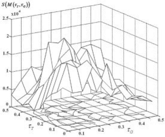
Provided with the above enrichment score, the optimal thresholds are determined to maximize the score. Figure 1 depicts an example of the score versus the threshold to search the optimal thresholds, 2D grids are introduced to discretize search space and then exhaustive search is conducted on the grid point to determine the optimal solution. Other more sophisticated numerical optimization approaches could also be applied to enhance the efficiency. However, since we have good prior knowledge about the value range of the parameters, this simple 2D grid search is proven to be effective. (An efficient way to calculate P-value of Fisher's exact test is available in the Supplementary Material.)

Fig. 1.

Plot of enrichment score versus parameters and illustrations of 2D grids search of the optimal parameters. The horizontal axes stand for (τ_T, τ_G), and the vertical axis stands for the enrichment score S(M(τ_T, τ_G)). For the 2D grid search, starting from the same initial input gene set, different modules will be identified for every different parameters (τ_T, τ_G) on the grid point and the optimal module M* would be the one that has the largest enrichment score.

3 RESULT

3.1 Simulation

ECTDISA was first validated on simulated data. This data was constructed to mimic a microarray experiment that measures the expression profiles of 1000 genes at 15 sample times. Five TTMs, which may share same genes and fall into the coherent model (multiplicative model) (Madeira and Oliveira, 2004), were embedded, each containing 30–50 genes and lasting for a period of 4–10 time points. (Figs 4–6 are achieved when simulated temporal modules last for 8–10 samples. Similar conclusion could be drawn from experiment where modules last for a period of 4–6 samples, whose result is available in Supplementary Material.)

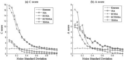
Fig. 4.

Performance VS Noise standard deviation. Performance of TDISA and K-means in terms of A score P_A and C score P_C for different noise level. ECTDISA and ECISA perform much better than ISA and K-means.

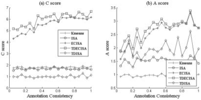
Fig. 6.

Impact of the consistence between prior knowledge and module. The consistent rate in horizontal axis is defined as the percentage of common genes that shared by the embedded module and the corresponding annotation gene category. This figure shows that the performance of ECTDISA when annotated gene category is not consistent with the embedded modules, i.e. not all genes involved in an annotated pathway behaves similarly. Simulation result shows ECTDISA is very robust towards the annotation files.

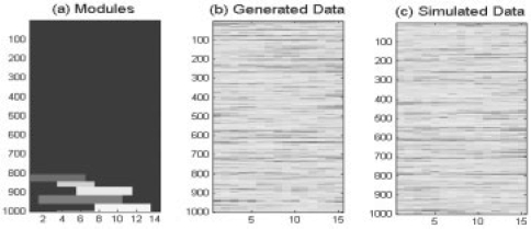
The module templates are shown in Figure 2a.

Fig. 2.

Data Generation. (a) Five TTMs are randomly generated. (b) Expression data is generated accordingly. (c) Reshuffle to get simulated data.

The data pattern of each module was generated according to an AR (1) model:X_mt=0.9X_m(t−1)+ε_mt, where, X_mt represents the expression level of module m at time t, ε_mt ∼ Normal (0, 1²). After this, the expression level of gene g at time t, can be simulated as:

.where, Normal (0, 1²). Then, each row of matrix X is multiplied with a random number that is generated from Normal (0, 0.4²); this is used to simulate the difference in expression strength among genes. Finally, Gaussian additive noise was applied (Fig. 2b), rows was shuffled to simulate real biological data, as Figure 2c.

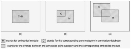
Meanwhile, a simulated annotation database was also constructed according to embedded modules. The database contains 10 gene categories, and each gene category contains a set of genes. There are five gene categories corresponding to five embedded modules, and the other five gene categories contain randomly selected genes. This is to simulate the reality that annotation database may contain both informative and uninformative knowledge. Regarding generating the gene categories that are corresponding to an embedded module, different strategies were applied (Fig. 3).

Fig. 3.

Simulated annotation database. (a) Ideal annotation database: annotated gene category contains exactly the same genes as embedded module. This is the case when we have ideal annotation databases. (b) Incomplete database: only parts of genes in an embedded module are annotated. This is the case when not all genes are annotated. (c) Incomplete and noised database: annotated gene category and the corresponding embedded module have overlap. It implies that not all genes are annotated; some annotations might be inaccurate or unsuitable to the specific data. This is a common case.

In order to evaluate the performance of ECTDISA, we introduce two measurements: A score P_A and C score P_C, i.e.

where |M| is the number of identified clusters, |T| is the number of true embedded modules in the data matrix, P_Tj, M_m is the enrichment P-value of a true embedded module T_j in the identified cluster

A score P_A is defined as the average of the largest enrichment scores of all the identified clusters. It indicates how likely a cluster identified by ECTDISA is a real embedded module. C score P_C is defined as the average of the largest enrichment scores of all the embedded true modules. P_C indicates whether all embedded modules are identified accurately by ECTDISA. In the following experiments, to obtain an A score or C score for any tested algorithm at any test condition, the algorithm is run on independent datasets until a stable score can be achieved.

In the first experiment, we evaluated impact of the noise effect on the performance of ECTDISA. A score P_A and C score P_C of ECTDISA were evaluated under different noise variance and they were also compared with those of the ISA algorithm (Bergmann et al., 2003) and K-means algorithm, which is a simple and widely used one way clustering approach. K-means clustering result is obtained by collecting all resulting modules from running K-means clustering 10 times using k = {1, 2,…,10}. In order to illustrate the contributions of time dependency and enrichment frame work, respectively, we also construct an algorithm ECISA, which use ECF to optimize parameters of ISA but without considering time dependency. We used an ideal annotation database as Figure 3a. Five additional functional categories were also constructed, each containing 30–50 randomly selected genes. The results were shown in Figure 4. We noticed that both C and A scores of ECTDISA, ISA and ECISA decreases with increase of noise level. Compared with ISA, ECTDISA and ECISA have much better performance, especially when noise level is low; while the performance of ECISA and ECTDISA are quite similar, which suggests that the improvement mainly accounts for ECF on this occasion. We also notice that even when the noise is close to 0, K-means cannot achieve satisfactory C and A scores, and its performance stays almost constant with noise level. This suggests that K-means cannot retrieve TTMs.

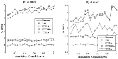
Next, we evaluated the impact of annotation database. First, we considered a scenario where only a fraction of genes in a module have functional annotation, for example, only 30% genes, while the rest have no annotation. The annotation is generated by strategy 2 in Figure 3b. The results were shown in Figure 5. Though ECTDISA tends to perform better when having complete prior knowledge, it still can provide good performance when only 30% of genes are annotated. This experiment demonstrated the ability of ECTDISA to uncover function of un-annotated genes based on expression and partial prior knowledge.

Fig. 5.

Impact of prior biological knowledge. When noise SD is 0.3, the two plots show the performances of the four algorithms when annotation file is not complete, i.e. not all genes are annotated. The horizontal axis represents the percentage of annotated genes. It shows, although more complete annotation can help to identify modules more accurately, the algorithm ECTDISA can still perform very well without complete annotations.

Then, we considered another more realistic situation, where embedded modules are not consistent with prior knowledge, i.e. annotation is incomplete and contains error, or not suitable to the specific data. We simulated the scenario by only assigning a function category to a fraction of genes in an embedded module and replace the other genes by randomly selected genes. This corresponds to strategy 3 in Figure 3c. The results were shown in Figure 6. We see that compared with ECISA, ECTDISA can retrieve modules more accurately especially when annotation database is not highly consistent with embedded modules, which is also a real situation. This implies the ability of ECTDISA to uncover new modules from functional related known modules. To summarize, it can be seen that, first, compared with ISA, time dependency does improve A score of the clustering significantly (Figs 4–6). This implies time dependency reduces significantly false positive components. Second, when the annotation database is not ideal (or consistent with real embedded module), ECTDISA outperforms ECISA in terms of both A and C scores, especially when annotation database is highly noisy (Fig. 6).

3.2 Test on yeast cell cycle dataset

We applied ECTDISA algorithm to the yeast cell cycle data in Spellman et al. (1998) obtained with equal sampling rate. The result is compared with ISA with GO enrichment analysis (Table 1). It can be seen that, although ECTDISA identifies less number of modules than ISA does, more GO terms are significantly enriched in ECTDISA result, which indicates that ECTDISA uncovers more significant functions. Further, on average, there are more GO terms significantly enriched in each module for ECTDISA than for ISA. It means that ECTDISA is more efficient in uncovering significant functions. To sum up, although ISA algorithm has been shown to be able to identify a number of biologically meaningful modules on the same data, ECTDISA apparently performs much effectively and more efficiently by uncovering a wider range of biological functions with less number of modules.

Table 1.

Comparison of ECTDISA and ISA on yeast cell cycle data

	Number of	Number of	Average number of
	identified	significantly enriched	significantly enriched GO Terms
	modules	GO Term (P-value	in each module
		< 10−10	P-value <10−10
ISA	192	179	0.93
ECTDISA	64	210	3.28

Detailed result is available in the Supplementary Material.

In Figure 12 of the Supplementary Material, we also observe both temporal and constant modules. For instance, a constant module (C59) apparently has a cyclic behavior, and is enriched by GO term ‘cell cycle’, and C48 is a temporal module significantly enriched with GO:002613 (P-value < 10⁻³⁴. A 10-fold cross validation is also conducted to evaluate ECTDISA's ability of finding meaningful transcription modules, and the detailed result is available in the Supplementary Material.

3.3 Test on Kaposi's sarcoma-associated herpesvirus infection data

We applied the ECTDISA algorithm to analyze the human time series microarray data derived from Kaposi's sarcoma-associated herpesvirus (KSHV) infection of human primary endothelial cells (Gao et al., 2003). The data were produced with Affymetrix Human Genome U133A Chips, consisting of the expression sample at time t=[0, 1, 3, 6, 10, 16, 24, 36, 54, 78] (hour) after infection. Since priority was given to earlier states, sample times were unevenly chosen.

3.3.1 Preprocessing and post processing

The 19 142 features (probe set ID) of total 22 383 have corresponding official gene symbol; 19 142 features with corresponding gene symbols are further merged into 11 945 genes by taking the maximum value of all corresponding probe set IDs. An intensity filter (the intensity of a gene should be above 100 in at least one sample), and a variance filter (the inter-quartile range of log2-intensities should be at least 0.2) were then applied to select 3825 differentially expressed genes along with their expression profile in original scale. Normalization is further applied to make all remaining genes contributing equally to the algorithm.

For the similarity measure ρ, Euclidean distance is applied to the first order time difference of expression profile rather than normalized data, which was introduced as a measure of trend of expression. Clustering was applied on time difference because we believe co-regulated genes should have similar trend instead of similar expression level.

Post-processing concerns merging similar modules (which is defined in the Supplementary Material). If two modules are consider similar, then the one has a smaller enrichment score will be eliminated. Since the parameters might be different for modules identified, there are modules in final result that are very similar in shape but not in enrichment scores and the gene contents. We believe that such modules reflect different biological functional groups and thus should be considered as different.

3.3.2 Result

The canonical pathways of the Molecular Signatures Database was adopted as prior knowledge (Subramanian et al., 2005), based on which enrichment score is calculated by Fisher's exact test. The optimal module was obtained by searching the 2D grids (τ_T, τ_G) for τ_T=[0.05:0.05:0.5], τ_G=[0.05:0.05:0.5]. The window size of the ECTDISA was W =3. After post processing, 48 modules were identified and normalized expression levels of the modules are shown in Figure 8 of the Supplementary Material. The top enriched pathways for M48 were enlisted in Table 2.

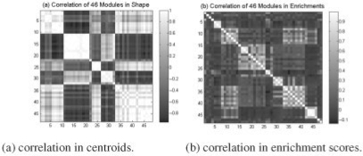
Fig. 8.

Correlation of modules. The figures shows the 2-way K-means clustering results of the correlations.

Table 2.

The most enriched three pathways in 48th module (M48)

Pathway name	Pathway annotation	−Lg(p)
HIFPATHWAY	Under normal conditions, hypoxia inducible factor HIF-1 is degraded; under hypoxic conditions, it activates transcription of genes controlled by hpoxic response elements	3.81
DREAMPATHWAY	The transcription factor DREAM blocks expression of the prodynorphin gene, which encodes the ligand of an opioid receptor that blocks pain signaling	3.6
BLADDER_CANCER	Genes involved in bladder cancer	3.40

For complete result, please refer to Supplementary Material.

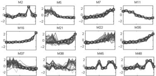
From the figures, we noticed that ECTDISA can uncover not only temporal transcriptional, but also constant time modules. The features of temporal module were clearly shown by the result. The 21st module (M21) in Figure 7 depicts a very good example, where genes of the module behave quite differently in first four samples but share a common trend afterwards. Similar behavior can be captured in most of the modules including M5, M22 and M37. However, at the same time, we also noticed that ECTDISA is not restricted for just temporal modules; a number of constant modules such as M2, M11 and M16 were also successfully retrieved, where genes behave similarly from the beginning to the end.

Fig. 7.

Selected modules (M2, 5, 7, 11, 16, 21, 22, 35, 37, 38, 45, 48).

We also observed that several modules are very similar in shape (e.g. M7, M16 and M35); however, a close examination of pathway enrichment revealed that these modules were enriched by different annotated pathways. To further examine this phenomenon, the correlations of centroids of modules and those of the enrichment scores were calculated and a 2-way K-means clustering of the correlations are displayed in Figure 8. Although Figure 8a suggests that a lot of modules are similar in shape, Figure 8b, in contrast, reveals that they are not similar in enrichement score and are actually enriched by different pathways, thus potentially reflecting different biological facts. Shape is not the only important factor to identify an informative module, it is also of crucial importance to select the right size (threshold) that can better address the related biological problem. ECTDISA can capture all these similar modules because it searches using different parameters. If (τ_T, τ_G) are fixed (like ISA), only one module in this group (M7, M16 and M35) can be identified and all other equivalent informative modules might be lost.

Among all the modules, the expression pattern of cellular genes in module M48 is relatively tight, and has an overall increased expression trend except the last time point (78 hpi) when KSHV undergoes full lytic replication (Gao et al., 2003; Yoo et al., 2005). This module consists of 13 enriched pathways (Table 1; for details, please refer to Supplementary Material), several of which have previously been shown to be upregulated following KSHV infection, including the HIF PATHWAY, IL6PATHWAY, ST_STAT3_ PATHWAY and ETS PATHWAY (Carroll et al., 2006; Punjabi et al., 2007; Xie et al., 2005; Ye et al., 2007). The fact that these pathways are clustered together and behave in tight range suggesting that they might be regulated by similar mechanism(s). However, further experimental examination is needed to confirm these observations.

4 DISCUSSION

ECTDISA is a new approach to analyze large-scale time-series gene microarray datasets. We discuss next a few distinct features of ECTDISA.

First, a sliding time window is used to consider the time dependency between samples by adding information from time adjacent samples and constraining the continuity of modules in time dimension. The use of this time window is based on the fact that the information from previous and latter samples could help make decision for a current sample. The window size W = 2L + 1 defines how much information from adjacent points you want to include into the analysis of a local time sample. The amount should be directly dependent on the sample interval and the changing speed of cell state. Presumably, if sample intervals are long and cell state changes fast, which result in less correlated samples, a smaller window should be used and vice versa. As a result of this sliding window, time-dependent modules that are only co-expressed for a short period of time can be uncovered. However, it does not exclude ECTDISA's ability to also retrieve modules of long-time span; many such modules can be observed in Figure 5.

Second, enrichment analysis is used as a guidance of module search, which helps to identify modules that are most likely to be biologically meaningful by choosing the optimal parameters for the algorithm. Embedded modules might not be identified accurately due to ad hoc choice parameters (τ_T, τ_G). ECF essentially serves as a result filter by removing thousands of modules that are not considered significant according to prior knowledge, keeping only a considerably small number of significant ones. The idea of obtaining an enrichment result has been a focus of recent computational biology research. Compared with the wide-used GSEA, this work represents an effort to extend such concept to clustering analysis. An interesting result that we want to emphasize is that, the ECTDISA is not sensitive to the selection of previous knowledge; even when the genes are not all annotated, and the annotated modules are not highly consistent with embedded modules, such annotation can still help. Moreover, as suggested by Figure 8, ECTDISA can further divide the co-expressed modules into functional sub-groups.

Third, when annotation database is not highly consistent with real modules, wrong decision could be made in ECF and thus it will be of crucial importance to provide only accurate result to ECF. We showed that time dependency can also help reduce the impact of inconsistency (Figs 5 and 6) and this is also the case when real data was analyzed. These experiments suggest that ECTDISA is a useful tool for uncovering gene functions.

4.1 Limitations

First, an optimal window size is still open questions. For the specific dataset used here, we reasonably assume that the dependency between each pair of adjacent samples is the same even though the samples are unevenly placed. The case of unequally sampling rate is apparently a very complicated issue deserving more investigation. We provide more discussion on the issue and proposed a possible solution in the Supplementary Material. Second, a potentially better approach to define the enrichment score is to consider only the top several enriched gene categories. Third, the efficiency of the search of optimal parameters can be further improved by employing sophisticated numerical optimization algorithms. They will be the focus of our future work.

Funding: NSF (grant CCF-0546345 to Y.H.); National Institutes of Health (grants CA096512 and CA124332 to S.-J.G.).

Conflict of Interest: none declared.

REFERENCES

- Alon U, et al. Broad patterns of gene expression revealed by clustering analysis of tumor and normal colon tissues probed by oligonucleotide arrays. Proc. Natl Acad. Sci. USA. 1999;96:6745–6750. doi: 10.1073/pnas.96.12.6745. [DOI] [PMC free article] [PubMed] [Google Scholar]
- Ashburner M, et al. Gene ontology: tool for the unification of biology. The Gene Ontology Consortium. Nat. Genet. 2000;25:25–29. doi: 10.1038/75556. [DOI] [PMC free article] [PubMed] [Google Scholar]
- Bergmann S, et al. Iterative signature algorithm for the analysis of large-scale gene expression data. Phys Rev. E Stat. Nonlin. Soft. Matter Phys. 2003;67:031902. doi: 10.1103/PhysRevE.67.031902. [DOI] [PubMed] [Google Scholar]
- Bittner M, et al. Data analysis and integration: of steps and arrows. Nat. Genet. 1999;22:213–215. doi: 10.1038/10265. [DOI] [PubMed] [Google Scholar]
- Califano A, et al. Analysis of gene expression microarrays for phenotype classification. Proc. Int. Conf. Intell. Syst. Mol. Biol. 2000;8:75–85. [PubMed] [Google Scholar]
- Carroll PA, et al. Latent Kaposi's sarcoma-associated herpesvirus infection of endothelial cells activates hypoxia-induced factors. J. Virol. 2006;80:10802–10812. doi: 10.1128/JVI.00673-06. [DOI] [PMC free article] [PubMed] [Google Scholar]
- Cheng Y, Church GM. Biclustering of expression data. Proc. Int. Conf. Intell. Syst. Mol. Biol. 2000;8:93–103. [PubMed] [Google Scholar]
- Dennis G, et al. DAVID: Database for Annotation, Visualization, and Integrated Discovery. Genome Biol. 2003;4:3. [PubMed] [Google Scholar]
- Eisen MB, et al. Cluster analysis and display of genome-wide expression patterns. Proc. Natl Acad. Sci. USA. 1998;95:14863–14868. doi: 10.1073/pnas.95.25.14863. [DOI] [PMC free article] [PubMed] [Google Scholar]
- Fuhrken PG, et al. Comparative, genome-scale transcriptional analysis of CHRF-288-11 and primary human megakaryocytic cell cultures provides novel insights into lineage-specific differentiation. Exp. Hematol. 2007;35:476–489. doi: 10.1016/j.exphem.2006.10.017. [DOI] [PubMed] [Google Scholar]
- Gao SJ, et al. Productive lytic replication of a recombinant Kaposi's sarcoma-associated herpesvirus in efficient primary infection of primary human endothelial cells. J. Virol. 2003;77:9738–9749. doi: 10.1128/JVI.77.18.9738-9749.2003. [DOI] [PMC free article] [PubMed] [Google Scholar]
- Gasch AP, Eisen MB. Exploring the conditional coregulation of yeast gene expression through fuzzy k-means clustering. Genome Biol. 2002;3 doi: 10.1186/gb-2002-3-11-research0059. RESEARCH0059. [DOI] [PMC free article] [PubMed] [Google Scholar]
- Getz G, et al. Coupled two-way clustering analysis of gene microarray data. Proc. Natl Acad. Sci. USA. 2000;97:12079–12084. doi: 10.1073/pnas.210134797. [DOI] [PMC free article] [PubMed] [Google Scholar]
- Hartigan JA. Direct clustering of a data matrix. J. Am. Stat. Assoc. (JASA) 1972;67:123–129. [Google Scholar]
- Ihmels J, et al. Revealing modular organization in the yeast transcriptional network. Nat. Genet. 2002;31:370–377. doi: 10.1038/ng941. [DOI] [PubMed] [Google Scholar]
- Ji L, Tan KL. Identifying time-lagged gene clusters using gene expression data. Bioinformatics. 2005;21:509–516. doi: 10.1093/bioinformatics/bti026. [DOI] [PubMed] [Google Scholar]
- Kanehisa M, et al. KEGG for linking genomes to life and the environment. Nucleic Acids Res. 2008;36:D480–D484. doi: 10.1093/nar/gkm882. [DOI] [PMC free article] [PubMed] [Google Scholar]
- Kloster M, et al. Finding regulatory modules through large-scale gene-expression data analysis. Bioinformatics. 2005;21:1172–1179. doi: 10.1093/bioinformatics/bti096. [DOI] [PubMed] [Google Scholar]
- Lazzeroni L, Owen A. Plaid models for gene expression data. Statist. Sinica. 2002;12:61–86. [Google Scholar]
- Madeira SC, Oliveira AL. Biclustering algorithms for biological data analysis: a survey. IEEE/ACM Trans. Comput. Biol. Bioinform. 2004;1:24–45. doi: 10.1109/TCBB.2004.2. [DOI] [PubMed] [Google Scholar]
- Madeira SC, Oliveira AL. Proceedings of the 5th Workshop on Algorithms in Bioinformatics (WABI'05). Mallorca, Spain: 2005. A Linear Time Biclustering Algorithm for Time Series Gene Expression Data; pp. 39–52. [Google Scholar]
- Owen AB, et al. A gene recommender algorithm to identify coexpressed genes. C. elegans. Genome Res. 2003;13:1828–1837. doi: 10.1101/gr.1125403. [DOI] [PMC free article] [PubMed] [Google Scholar]
- Prelic A, et al. A systematic comparison and evaluation of biclustering methods for gene expression data. Bioinformatics. 2006;22:1122–1129. doi: 10.1093/bioinformatics/btl060. [DOI] [PubMed] [Google Scholar]
- Punjabi AS, et al. Persistent activation of STAT3 by latent Kaposi's sarcoma-associated herpesvirus infection of endothelial cells. J. Virol. 2007;81:2449–2458. doi: 10.1128/JVI.01769-06. [DOI] [PMC free article] [PubMed] [Google Scholar]
- Reiss DJ, et al. Integrated biclustering of heterogeneous genome-wide datasets for the inference of global regulatory networks. BMC Bioinformatics. 2006;7:280. doi: 10.1186/1471-2105-7-280. [DOI] [PMC free article] [PubMed] [Google Scholar]
- Sheng Q, et al. Biclustering microarray data by Gibbs sampling. Bioinformatics. 2003;19(Suppl 2):ii196–ii205. doi: 10.1093/bioinformatics/btg1078. [DOI] [PubMed] [Google Scholar]
- Spellman PT, et al. Comprehensive identification of cell cycle-regulated genes of the yeast Saccharomyces cerevisiae by microarray hybridization. Mol. Biol. Cell. 1998;9:3273–3297. doi: 10.1091/mbc.9.12.3273. [DOI] [PMC free article] [PubMed] [Google Scholar]
- Subramanian A, et al. Gene set enrichment analysis: a knowledge-based approach for interpreting genome-wide expression profiles. Proc. Natl Acad. Sci. USA. 2005;102:15545–15550. doi: 10.1073/pnas.0506580102. [DOI] [PMC free article] [PubMed] [Google Scholar]
- Supper J, et al. EDISA: extracting biclusters from multiple time-series of gene expression profiles. BMC Bioinformatics. 2007;8:334. doi: 10.1186/1471-2105-8-334. [DOI] [PMC free article] [PubMed] [Google Scholar]
- Tamayo P, et al. Interpreting patterns of gene expression with self-organizing maps: methods and application to hematopoietic differentiation. Proc. Natl Acad. Sci. USA. 1999;96:2907–2912. doi: 10.1073/pnas.96.6.2907. [DOI] [PMC free article] [PubMed] [Google Scholar]
- Tanay A, et al. Discovering statistically significant biclusters in gene expression data. Bioinformatics. 2002;18(Suppl 1):S136–S144. doi: 10.1093/bioinformatics/18.suppl_1.s136. [DOI] [PubMed] [Google Scholar]
- Xie J, et al. Kaposi's sarcoma-associated herpesvirus induction of AP-1 and interleukin 6 during primary infection mediated by multiple mitogen-activated protein kinase pathways. J. Virol. 2005;79:15027–15037. doi: 10.1128/JVI.79.24.15027-15037.2005. [DOI] [PMC free article] [PubMed] [Google Scholar]
- Ye FC, et al. Kaposi's sarcoma-associated herpesvirus promotes angiogenesis by inducing angiopoietin-2 expression via AP-1 and Ets1. J. Virol. 2007;81:3980–3991. doi: 10.1128/JVI.02089-06. [DOI] [PMC free article] [PubMed] [Google Scholar]
- Yoo SM, et al. Early and sustained expression of latent and host modulating genes in coordinated transcriptional program of KSHV productive primary infection of human primary endothelial cells. Virology. 2005;343:47–64. doi: 10.1016/j.virol.2005.08.018. [DOI] [PMC free article] [PubMed] [Google Scholar]
- Zhang Y, et al. Proceedings of the International Conference on Information Technology: Coding and Computing (ITCC'05) - Volume I - Volume 01. Las Vegas, Nevada, USA: 2005. A Time-Series Biclustering Algorithm for Revealing Co-Regulated Genes. IEEE Computer Society. [Google Scholar]