A model of higher accuracy for the individual haplotyping problem based on weighted SNP fragments and genotype with errors

Abstract

Motivation: In genetic studies of complex diseases, haplotypes provide more information than genotypes. However, haplotyping is much more difficult than genotyping using biological techniques. Therefore effective computational techniques have been in demand. The individual haplotyping problem is the computational problem of inducing a pair of haplotypes from an individual's aligned SNP fragments. Based on various optimal criteria and including different extra information, many models for the problem have been proposed. Higher accuracy of the models has been an important issue in the study of haplotype reconstruction.

Results: The current article proposes a highly accurate model for the single individual haplotyping problem based on weighted fragments and genotypes with errors. The model is proved to be NP-hard even with gapless fragments. Based on the characteristics of Single Nucleotide Polymorphism (SNP) fragments, a parameterized algorithm of time complexity O(nk₂2^k₂ + m log m + mk₁) is developed, where m is the number of fragments, n is the number of SNP sites, k₁ is the maximum number of SNP sites that a fragment covers (no more than n and usually smaller than 10) and k₂ is the maximum number of the fragments covering a SNP site (usually no more than 19). Extensive experiments show that this model is more accurate in haplotype reconstruction than other models.

Availability: The program of the parameterized algorithm can be obtained by sending an email to the corresponding author.

Contact: jxwang@mail.csu.edu.cn

1 INTRODUCTION

The different DNAs between two individuals’ genomes account for about 0.5% of the whole genome sequence (Levy et al., 2007), and these differences make the two individuals different from each other in figures, diseases susceptibilities and other phenotypes. A single nucleotide polymorphism (SNP) is a change of a single nucleotide in a given position of the genome sequence with a frequency not <1% in a given population. There are millions of SNPs in the human genome (The International HapMap Consortium, 2005; Venter et al., 2001). SNPs are believed to be the major genetic cause to human phenotypic variability.

It is widely accepted that at a given SNP site, there are only two possible nucleotides, one usually occurs in more than 90% individuals of a population and is called major allele, and the other is called minor allele. For briefness, a SNP is represented by 0, or 1, instead of a nucleotide (A, C, G or T), where ‘0’ denotes the major allele (at the SNP site), and ‘1’ denotes the minor allele.

The human genome is made up of 23 pairs of chromosomes. A sequence of SNP alleles on one of a pair of chromosomes is called a haplotype, which can be denoted by a string over {0, 1}. A sequence of conflated (unordered pair of) SNP alleles at each SNP site of a pair of homologous chromosomes is called a genotype. A genotype can be represented by a string over {0, 1, 2}, where ‘0’ (resp. ‘1’) indicates that both SNPs are ‘0’ (resp. ‘1’) at the same SNP site of the pair of chromosomes, and ‘2’ indicates that at the same SNP site, the SNP on one of the pair of chromosomes is ‘0’, while on the other of the pair is ‘1’.

In Figure 1, the haplotypes of the individual are (A, C, G, T) and (G, C, C, T), which can be denoted by ‘0100’ and ‘1110’. The genotype is (A/G, C/C, G/C, T/T), which can be denoted by ‘2120’.

Fig. 1.

Haplotypes

In finding susceptibility loci for complex diseases, haplotype-based methods are more powerful and robust than the methods based on individual SNPs (Akey et al., 2001). However, determining haplotypes using biological techniques is both time consuming and expensive, and is much harder than determining individual SNPs or genotypes. Therefore, to reduce the cost of determining haplotypes, effective computational methods have been in demand.

There have been many computational models for the haplotyping problem (Adkins, 2004; Bonizzoni et al., 2003; Zhang et al., 2006), and they generally fall into two classes: individual haplotyping and population haplotyping. The individual haplotyping problem is concerned with assembling a pair of haplotypes from an individual's aligned DNA fragments, while the population haplotyping problem is to infer the haplotypes of a sample of people in a population from their genotypes.

This current article is focused on the individual haplptyping problem and aimed at studying highly accurate model and developing effective computational algorithms for the problem. The article is organized as follows. In Section 2, we introduce the individual haplotyping problem and propose a new model based on weighted SNP fragments and genotype with errors. We prove that the individual haplotyping problem under this model is NP-hard. To effectively solve the problem under this model, we develop in Section 3 an exact parameterized algorithm for the problem. Section 4 presents experimental results and discussions. The article is concluded by Section 5.

2 FORMULATION AND PROBLEMS

2.1 The individual haplotyping problem

For large-scale haplotyping, a set of aligned SNP fragments from a pair of chromosomes can be generated by DNA shotgun sequencing or other sequencing experiments. The individual haplotyping problem (Lancia et al., 2001) is aimed at partitioning the set of SNP fragments into two subsets, each determining a haplotype.

To formulate the problem, we introduce some notations and concepts, similar to those used in Xie and Wang (2007).

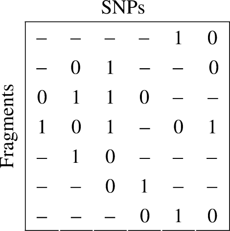
In the following discussion, m aligned SNP fragments coming from a pair of chromosomes with n SNP sites are represented by an m×n SNP matrix M over the alphabet {0, 1, −}, in which each row corresponds to a fragment and each column corresponds to a SNP site. The SNP allele of the ith fragment at the jth SNP site is denoted by the entry M_i,j of M at the ith row and the jth column, and the entry M_i,j takes value ‘−’ if either the ith fragment does not cover the jth SNP site or the corresponding SNP allele of the ith fragment cannot be determined with enough confidence.

We say that the ith row covers the jth column if either M_i,j≠‘−’, or there are two indices k and r such that k<j<r and both M_i,k and M_i,r are not ‘−’.

The set of (ordered) rows covering the jth column is denoted by R_s(j). The first column that the ith row covers is denoted by l(i), and the last column that the ith row covers is denoted by r(i).

As an example, in the SNP matrix in Figure 2, row 2 covers columns 2, 3, 4, 5 and 6, and R_s(5)={1, 2, 4, 7}.

Fig. 2.

A SNP matrix.

If M_i,j takes the value ‘0’ and M_k,j takes the value ‘1’, or M_i,j takes the value ‘1’ and M_k,j takes the value ‘0’, we say that the ith row and the kth row of M conflict at the column j. If two rows of M do not conflict at any column, we say that they are compatible.

If the rows of a SNP matrix M can be partitioned into two subsets such that the rows in each subset are all compatible, then we say that the SNP matrix M is feasible.

Obviously, a SNP matrix M is feasible if and only if there are two haplotypes such that every row of M is compatible with one of the two haplotypes. In this case, we say that the SNP matrix M can be derived from the two haplotypes.

Since a row of M comes from one of a pair of chromosomes, if there are no DNA sequencing errors, we can always derive M from the haplotypes of the pair of chromosomes. However, DNA sequencing errors are unavoidable and it is hard to decide which copy of chromosome a SNP fragment comes from. This has made the individual haplotyping problem complicated.

Based on different optimal criteria, various computational models have been proposed for the problem. Some typical models include (Lancia et al., 2001; Lippert et al., 2002): Minimum fragment Removal (MFR), Minimum SNPs Removal (MSR) and Minimum Error Correction (MEC). Among these models, MEC is considered to have most biological meaning. MEC is also called Minimum Letter Flips (MLF) (Greenberg et al., 2004) and has been extended to include different extra information.

A DNA sequencer can provide a confidence level for each base, which is the probability that the base was correctly read (Zhao et al., 2005). The confidence levels for an m×n SNP matrix M can be represented as an m×n weight matrix W, in which the element W_i,j of W at row i and column j is the confidence level of the value M_i,j. We also define W_i,j=0 if M_ij= ‘−’. By including a weight matrix, Greenberg et al. (2004) introduced the weighted minimum letter flips (WMLF) model, and Zhao et al. (2005) formulated it as follows:

Weighted Minimum Letter Flips (WMLF): Given a SNP matrix M and the corresponding weight matrix W, flip a number of elements in M (‘0’ into ‘1’ and vice versa) so that the resulting matrix is feasible and the sum of the elements in W corresponding to the flipped elements in M is minimized.

An individual's genotype can be phased relatively easily. Wang et al. (2005) extended the MEC model as follows:

MEC with Genotype Information (MEC/GI): Given a SNP matrix M and a genotype G, flip a minimum number of elements in M (‘0’ into ‘1’ and vice versa) so that the resulting matrix can be derived by two haplotypes that make up the genotype G.

In general, WMLF and MEC/GI are superior to MEC (or MLF) in the accuracy of haplotype reconstruction. However, WMLF does not take genotype information into account, and MEC/GI does not consider the errors in a genotype and the confidence levels of DNA bases. In fact, there are always genotyping errors. In order to improve the accuracy of haplotype reconstruction, we propose a new model in the next subsection.

2.2 WMLF incorporating genotyping uncertainty

There are two broad categories of genotyping errors (Kang et al., 2004): operational errors and genotype scoring errors. Recently, the operational errors have decreased significantly in high-throughput genotyping due to biological technology advances. On the other hand, genotype scoring errors are still a significant challenge for automated scoring softwares (Kang et al., 2004), and research on kernel algorithms for genotype scoring remains a hot spot (Carvalho et al., 2007; Xiao et al., 2007). Limited by scoring softwares, genotyping errors are unavoidable (Kang et al., 2004; Zhu, 2006). Therefore, incorporating genotyping uncertainty will help the process of reconstructing haplotypes.

To incorporate genotyping uncertainty, Kang et al. (2004) introduced GenoSpectrum. Considering n SNPs of a individual, a GenoSpectrum F is a 3×n matrix as given in Figure 3, where for each j, 1≤j≤n,f_0,j,f_1,j,f_2,j are the likelihood that the individual's genotype at the jth SNP site is 0, 1 and 2, respectively.

Fig. 3.

GenoSpectrum.

Let H[j] and G[j] denote the jth character of a haplotype H and a genotype G, respectively.

DEFINITION 1. —

Let M be an m × n SNP matrix and let F be a 3 × n GenoSpectrum. The most likely genotype G_M,F of M with respect to F is defined to be the genotype whose values satisfy the following conditions for all j:

Roughly speaking, G_M,F[j] gives an index h so that the value f_h,j shows the degree of consistency of the jth column of the SNP matrix M and the jth column of the GenoSpectrum F. In particular, if all elements in the jth column of M are ‘−’, then the SNP matrix M provides no information for the jth SNP site. Thus, the largest value f_k,j in the jth column of F, where k=G_M,F[j], shows the degree of confidence that the ‘most likely’ genotype of the jth SNP site is k. If there are both 0's and 1's in the jth column of M, then G_M,F[j]=2 and the value f_2,j is the degree of confidence that the jth column in the SNP matrix M and the jth column in the GenoSpectrum F are consistent. Finally, if the jth column in the SNP matrix M contains exactly one value q from {0, 1}, then G_M,F[j]=q and the value f_q,j is the degree of confidence that the jth column in the SNP matrix M and the jth column in the GenoSpectrum F are consistent.

DEFINITION 2. —

Let M be an m × n SNP matrix and let F be a 3 × n GenoSpectrum. The distance d(M, F) between M and F is defined as follows:

By the above discussion on the most likely genotype G_M,F of M with respect to F, we can see, intuitively, that the distance d(M,F) measures the degree of inconsistency between the SNP matrix M and the GenoSpectrum F.

DEFINITION 3. —

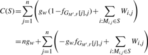
Let M be an m × n SNP matrix, W be an m × n weight matrix corresponding to M, F be a 3 × n GenoSpectrum, g_w be a weighted coefficient, S be an element subset of M (i.e. S⊆{M_i,j|1≤i≤m,1≤j≤n}), and M^′ be the SNP matrix derived from M by flipping the elements in S. The flipping cost of S based on g_w, M, W and F is defined as follows:

Since the value d(M′,F) measures the degree of inconsistency between the SNP matrix M′ and the GenoSpectrum F, the flipping cost C(S) of a subset S of elements in the SNP matrix M is measured in terms of two metrics: the degree of inconsistency between the resulting SNP matrix M′ and the GenoSpectrum F (i.e. d(M′,F)), and the degree of confidence that is decreased during flipping the elements in S (i.e. ∑_Mi,j∈SW_i,j). The weighted coefficient g_w is used to adjust the relationship between these two metrics.

Based on Definitions 2 and 3, the following equation holds true:

(1)

In the following, we propose a new computational model for the individual haplotyping problem.

WMLF/GS:

(Weighted Minimum Letter Flips with GenoSpectrum)

Given an m×n SNP matrix M, an m×n weight matrix W, a 3×n GenoSpectrum F and a weighted coefficient g_w, find a subset S of elements in M and flip the elements in S (‘0’ into ‘1’ and vice versa) so that the resulting matrix is feasible and the flipping cost of the subset S based on g_w, M, W and F is minimized.

It is easy to see that when the weighted coefficient g_w is set to 0, the WMLF/GS problem degenerates into the WMLF problem.

Let WMLF/GS(g_w,M,W,F) denote a solution to the WMLF/GS problem, i.e. an element subset S of M that minimizes C(S) under the condition that after flipping the elements in S,M is feasible.

THEOREM 1. —

The WMLF/GS problem is NP-hard even if its SNP matrix is gapless.

PROOF. —

The WMLF problem can be reduced from the weighted max-cut problem, which is a well-known NP-hard problem (Zhao et al., 2005). Similarly, the WMLF/GS problem can be reduced from the weighted max-cut problem.

The weighted max-cut problem is defined as follows: given a undirected graph G=(V,E) and a positive edge weight function w:E→ℝ₊, find a partition (V₁,V₂) of V such that the sum of the weights of the edges with one end in V₁ and the other end in V₂ is maximized. For briefness, the sum of the weights of the edges with one end in V₁ and the other end in V₂ will be called the cut weight of (V₁, V₂), and the weight of an edge (i,j) is denoted by w(i,j).

As an example, consider the graph G in Figure 4(a). Let V₁={1,4} and V₂={2,3}. Then the cut weight of (V₁, V₂) is 0.5+0.2+0.3+0.6=1.6. It can be easily verified that this cut has a maximum weight.

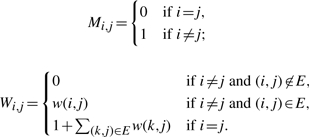
Given a undirected graph G=(V,E) with n vertices and a positive edge weight function w, where, without loss of generality, the vertices are named as 1, 2,…, n. We can construct an n×n SNP matrix M and a n×n weight matrix W as follows:

The 3×n GenoSpectrum F can be constructed as follows: for j=1,…,n,f_0,j=f_1,j=0, f_2,j=1. Let g_w be any positive number.

According to the rules above, the SNP matrix M and the corresponding matrix W constructed from the undirected weighted graph G in Figure 4a are given in Figure 4b (with the weight values given in the brackets), and the GenoSpectrum F is given in Figure 4c.

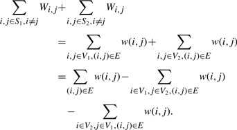
In general, for the SNP matrix M constructed above, the ith row represents the ith vertex of G, and a partition of V corresponds to a partition (S₁=V₁,S₂=V₂) of the rows of M. Let k be 1 or 2. To make the rows in S_k compatible with each other and minimize the sum of the weights of the flipped elements, for each row i∈S_k, all the elements of other rows in S_k at column i should flip from 1 to 0, in order not to conflict with row i at column i. Therefore, the minimum sum of the weights of the flipped elements is equal to ∑_{i,j∈Sk, i≠j}W_i,j. Consequently, we have:

Let the set of the flipped elements above be S. After flipping the elements in S the distance between M and F is 0. Therefore, C(S) is minimized if and only if the cut weight of (V₁,V₂) is maximized. This completes the proof of the theorem. ▪

In fact, most models for the individual haplotyping problem are NP-hard. To obtain exact solutions to these models, some dynamic programming and branch-and-bound algorithms have been proposed. For larger problem instances, these exact algorithms become infeasible, and heuristic algorithms have been used instead. However, heuristic algorithms usually cannot ensure accuracy. Recently, fixed-parameter tractability theory has been used to design practical exact algorithms for certain NP-hard problems with great success. For the MFR and MSR problems, Xie et al. (2007) and Xie and Wang (2007) have proposed parameterized algorithms by taking the advantage of the characters of SNP fragments. In the following section, we will use the technique to develop a parameterized algorithm for the WMLF/GS problem.

Fig. 4.

(a) A weighted graph. (b) A SNP matrix corresponding to the weighted graph in (a), with weighted values given in brackets. (c) A GenoSpectrum corresponding to the weighted graph in (a).

3 METHODS

In Xie and Wang (2007) and Xie et al. (2007), we have observed the following properties of DNA sequence fragment data. Due to technical limits, the sequencing instruments such as ABI 3730 and MageBACE in most big sequencing centers can only sequence DNA fragments whose length is usually not more than 1200 nucleotide bases. Since the SNP density is about 1 SNP per 1 kb, the maximum number of SNP sites that a fragment can cover is small.

Moreover, in DNA sequencing experiments, the fragment coverage is also small. In both Celera's whole-genome shotgun assembly of the human genome and the human genome project of the International Human Genome Sequencing Consortium, the fragment average coverage is about five (International Human Genome Sequencing Consortium, 2001; Venter et al., 2001). Although the fragment covering rate varies along the whole genome, the fragment coverage plot in Huson et al. (2001) about the fragment data of the human genome project of Celera's shows that the number of fragments covering a site is bounded by 19. Therefore, compared with the total number of fragments, the number of fragments that cover a SNP site is very small.

Based on the observations above, as in Xie and Wang (2007), we introduce the (k₁,k₂) parameterized condition.

DEFINITION 4. —

The (k₁,k₂) parameterized condition: a single fragment covers at most k₁ SNP sites, and the number of fragments that cover a SNP site is bounded by k₂.

As to the corresponding SNP matrix M, the (k₁,k₂) parameterized condition means that each row of M covers at most k₁ columns and each column of M is covered by at most k₂ rows.

For an m×n SNP matrix M, the parameters k₁ and k₂ can be obtained by scanning all rows of M. In the worst case, k₁=n and k₂=m. But as to the fragment data of Celera's human genome project, k₂ is no more than 19 (Huson et al., 2001).

3.1 A parameterized algorithm for WMLF/GS

In this subsection, the SNP matrix M is preprocessed as follows: sort the rows in M in ascending order such that for any two rows i₁ and i₂, if i₁<i₂, then l(i₁)≤l(i₂), which is similar to the preprocessing in Xie et al. (2007) and Xie and Wang (2007).

For a solution to the WMLF/GS problem for a SNP matrix M, after flipping the corresponding elements, all the rows of M can be partitioned into two classes H₀ and H₁, such that every two rows in the same class are compatible.

DEFINITION 5. —

Let R be a subset of rows in a SNP matrix M. A partition function P on R maps each row in R to one of the values {0, 1}.

Suppose that R contains h>0 rows, a partition function P on R can be denoted by an h-digit binary number in {0, 1}, where the ith digit is the P value of the ith row in R. If R=∅, we also define a unique partition function P, which is denoted by −1.

Recall that R_s(j) denotes the set of rows in the SNP matrix M that cover the jth column. For briefness, a partition function defined on R_s(j) is called a partition function at column j. For a SNP matrix M satisfying the (k₁,k₂) parameterized condition, there are at most 2^k₂ different partition functions at column j.

Let R be a set of rows of the matrix M, and P be a partition function on R. For a subset R′ of R, the partition function P′ on R′ obtained by restricting P on the subset R′ is called the projection of P on R′, and P is called an extension of P′ on R.

For briefness, let M(j) denote the set of all non-empty elements from column 1 to column j in M, and M[:,j] (W[:,j], or F[:,j]) denotes the SNP matrix (resp. the weighted matrix, or the GenoSpectrum) consisting of the first j columns of M (resp. W, or F).

DEFINITION 6. —

Fix a j. Let P be a partition function on a row set R. Defined V_E[P,j] to be any subset S of elements of M that satisfies the following conditions:

1. For each element M_r,k in S, 1≤k≤j}.

2. After flipping the elements of S, there is a partition (H₀,H₁) of all rows in M such that any two rows in the same class do not conflict at any column from 1 to j, and for any row i∈R, row i is in the class H_q if and only if P(i)=q, for q∈{0,1}.

DEFINITION 7. —

Fix a column index j. Let g_w be a weighted coefficient, M^′=M[:,j], W^′=W[:,j], F^′=F[:,j], P be a partition function at column j, and the collection of all possible subsets V_E[P,j] be 𝒱. Defined E[P,j]=min_S∈𝒱C(S) and S_E[P,j] to be any subset in 𝒱 that satisfies C(S_E[P,j])=E[P,j], where C(S) and C(S_E[P,j]) are the flipping costs of S and S_E[P,j], respectively, based on g_w, M^′, W^′, and F^′.

From Definitions 6 and 7, it is easy to verify that the following equation holds true:

(2)

where P is a partition function at column n that minimizes E[P,n].

Given a V_E[P,j], let M′ be the SNP matrix derived from M[:,j] by flipping the elements in V_E[P,j], and be the set of the elements of M that are in column l and in V_E[P,j]. Let denote , where G_M′,F[:,j][l] is the value at column l of the most likely genotype of M′, and f_{GM′, F[:, j][l],l} is the value of the element in F[:,j] at row G_M′,F[:,j][l] and column l. From Equation (1), the flipping cost of V_E[P,j] based on g_w, M[:,j], W[:,j] and F[:,j] can be calculated as follows: .

Given a partition function P at column j, the rows covering column j can be partitioned into (H₀,H₁) by P according to the following rule: for each row i∈R_s(j), i∈H_q if P(i)=q. In order to make the rows in the same class not conflict at column j, the values at column j of some rows may have to be flipped. For q∈{0, 1}, let v_q=0 or 1. For any row i∈H_q, if M_i,j=v_q, M_i,j is to be flipped. In consequence, we obtain a set Flips of flipped elements, and C_j(Flips)=∑_q=0,1∑_{i:i∈Rs(j), P(i)=q, Mi,j=vqWi,j−gwfGM′, F[:, j][j],j}, where M′ is the SNP matrix derived from M[:,j] by flipping the elements in Flips. Obviously, M′ is feasible.

Let g(v₀,v₁) be a map such that: if v₀=v₁=0, g(v₀,v₁)=1; if v₀=v₁=1, g(v₀,v₁)=0; and if v₀≠v₁, g(v₀,v₁)=2. Based on Definition 1, It is easy to see that G_M′,F[:,j][j]=g(v₀,v₁).

For k,v=0,1, let w(P,j,k,v) denote

Let Minor(P,j,0) and Minor(P,j,1) denote the value of v₀ and the value of v₁ that minimize w(P,j,0,v₀)+w(P,j,1,v₁)−g_w f_g(v0,v1),j, respectively. Let Flips(P,j) denote the set of the flipped elements {M_i,j∣M_i,j=Minor(P,j,P(i))}.

Fix a P and a j, it is obvious that is the minimum if and only if . Therefore, the following equations hold true.

(3)

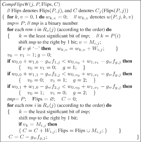
(4)

Figure 5 gives a function CompFlipsW(j,P,Flips,C) to compute Flips(P,j) and C_j(Flips(P,j)), whose time complexity is O(k₂) for a SNP matrix M satisfying the (k₁,k₂) parameterized condition.

In order to present our algorithm, we need to extend the above concepts from one column to two columns as follows. Let the set of all rows that cover both columns j₁ and j₂ be R_c(j₁,j₂).

Fig. 5.

CompFlipsW.

DEFINITION 8. —

Fix a j. Let g_w be a weighted coefficient, M^′=M[:,j], W^′=W[:,j], F^′=F[:,j], P^′ be a partition function on R_c(j,j+1), and the collection of all possible subsets V_E[P^′,j] be 𝒱. Defined B[P^′,j]=min_S∈𝒱C(S) and S_B[P^′,j] to be any element in 𝒱 that satisfies C(S_B[P^′,j])=B[P^′,j], where C(S) and C(S_B[^′,j]) are the flipping costs of S and S_B[P^′,j], respectively, based on g_w, M^′, W^′ and F^′.

Given a j and a partition function P^′ on R_c(j,j+1). If E[P,j] and S_E[P,j] are known for each extension P of P^′ on R_s(j), B[P^′,j] and S_B[P^′,j] can be calculated by the following equations:

(5)

(6)

Inversely, for any partition function P on R_s(j), because R_c(j−1,j) is a subset of R_s(j), the project P^′ of P on R_s(j) is unique. When S_B[P^′,j−1] and B[P^′,j−1] are known, E[P,j] and S_E[P,j] can be calculated according to the following equations, whose correctness can be proved similarly as that for Equations (3) and (4).

(7)

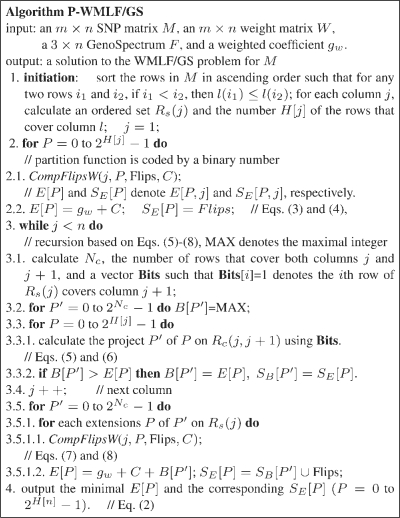
(8)

Based on Equations (2)-(8), the solution to the WMLF/GS problem for a SNP matrix M can be obtained as follows: first, E[P,1] and S_E[P,1] are obtained according to Equations (3) and (4) for all partition functions P at column 1; second, B[P′,1] and S_B[P′,1] can be obtained by using Equations (5) and (6) for all partition functions P′ on R_c(1,2); third, E[P,2] and S_E[P,2] can be obtained by using Equations (7) and (8) for all partition functions P on R_s(2); and so on. Finally, E[P,n] and S_E[P,n] can be obtained for all partition functions P at column n. Once E[P,n] and S_E[P,n] for all possible P are known, a solution to the WMLF/GS problem for M can be obtained by using Equation (2). See Figure 6 for the details of our P-WMLF/GS algorithm.

Fig. 6.

P-WMLF/GS algorithm.

THEOREM 2. —

If an m×n SNP matrix M satisfies the (k₁,k₂) parameterized condition, the P-WMLF/GS algorithm solves the WMLF/GS problem in time O(nk₂ 2^k₂+mlog m+mk₁) and space O(mk₁2^k₂+nk₂).

PROOF. —

Given an m×n SNP matrix M satisfying the (k₁,k₂) parameterized condition, consider the following data structure: each row keeps the first and the last column that the row covers, i.e. its left and right value, and its values at the columns from its left column to its right column. In such a data structure, M takes space O(mk₁). It is easy to see that R_s takes space O(nk₂), H takes space O(n), E and B take space O(2^k₂) and S_E and S_B take space O(mk₁₂^k₂). In summary, the space complexity of the algorithm is O(mk₁₂^k₂+nk₂).

Now we discuss the time complexity of the algorithm. In Step 1, sorting takes time O(mlogm). All R_ss can be obtained by scanning the rows only once, which takes time O(mk₁). For any column j, because no more than k₂ rows cover it, H[j]≤k₂, the function CompFlipsW takes time O(k₂), and Step 2 takes time O(k₂ 2^k₂). In Step 3.1, scanning R_s(j) and R_s(j+1) simultaneously can obtain N_c and Bits, and takes time O(k₂). Step 3.2 takes time O(2^k₂), and Step 3.3 takes time O(k₂ 2^k₂). In Step 3.5, for each P′, there are 2^H[j]−N_C extensions of P′ on R_s(j). Given P′, an extension of P′ can be obtained by a bit-or operation in time O(1), because after the sorting in Step 1, the rows that cover column j, but do not cover column j−1 are all behind the rows in R_c(j−1,j). In all, Step 3.5 takes time O(k₂ 2^{N_c 2k₂−N_c}). Then Step 3 is iterated n−1 times and takes time O(nk₂₂^k₂). Step 4 takes time O(2^k₂). In summary, the time complexity of the algorithm is O(nk₂₂^k2+mlogm+mk₁). This completes the proof of the theorem. ▪

4 EXPERIMENTAL RESULTS

We compare three models WMLF/GS, MEC/GI and WMLF for the individual haplotyping problem. For WMLF/GS, we adopt our P-WMLF/GS algorithm; for MEC/GI, we adopt Wang et al.'s genetic algorithm GA-MEC/GI (Wang et al., 2005); and for WMLF, we adopt Zhao et al.'s dynamic clustering algorithm DC-WMLF (Zhao et al., 2005). In the experiments, we compare the running time and the reconstruction rate of haplotypes (Wang et al., 2005) of these three algorithms. The reconstruction rate of haplotypes is defined as the ratio of the number of the SNP sites that are correctly inferred out by an algorithm to the total number of the SNP sites of the haplotypes.

The haplotype data can be obtained by two methods (Wang et al., 2005): the first is to get real haplotypes from public domain, and the second is to generate simulated haplotypes by computers. In our experiments, the real haplotypes were obtained from the file genotypes_chr1_CEU_r21_nr_fwd_phased.gz,¹ which was issued in July 2006 by the International HapMap Project (2005). The file contains 120 haplotypes on chromosome 1 of 60 individuals of the CEU with each haplotype containing 193 333 SNP sites. From the 60 individuals, select a individual at random. Then beginning with a random SNP site, a pair of haplotypes of a given length can be obtained from the haplotypes of the selected individual.

The simulated haplotypes can be generated as follows (Panconesi and Sozio, 2004; Wang et al., 2005). At first a haplotype h₁ of length n is generated at random, then another haplotype h₂ of the same length is generated by flipping every character of h₁ with a probability of d.

As to fragment data, to the best of our knowledge, real DNA fragments data in the public domain are not available, and references Wang et al. (2005) and Panconesi and Sozio (2004) used computer-generated simulated fragment data. After obtaining a pair of real or simulated haplotypes, in order to make the generated fragments have the same statistical features as the real data, a widely used shotgun assembly simulator Celsim (Myers, 1999 is invoked to generate m fragments whose lengths are between lMin and lMax. At last the output fragments are processed to plant reading errors with probability e_s and empty values with probability p.

In our experiments, the parameters are as follows: fragment coverage rate c=10, the difference rate between two haplotypes d=20%, the minimal length of fragment lMin=3, the maximal length of fragment lMax=7 and empty values probability p=2%.

The weight matrix W corresponding to the fragments is generated by the method of Zhao et al. (2005): the entries of w are normally distributed with mean μ and variance σ²=0.05. For a correct SNP site, μ=0.9, and for an error SNP site, μ=0.8.

The genotype without error can be obtained from the pair of haplotypes produced above. Since the genotyping error in biological assay is about 1% (Xiao et al., 2007), we plant some errors in the genotype (Zhu 2006) by changing the value of every char of the genotype with a probability e_g as follows: if the value is ‘0’ or ‘1’, it is changed to ‘2’; if the value is ‘2’, it is changed to ‘0’ or ‘1’ randomly. The GenoSpectrum F is generated as follows. For the column j at which the genotype is k: when k is correct, if k=0 (or 1),f_0,j (or f_1,j) is normally distributed with mean μ=0.9 and variance σ²=0.05, f_1,j (or f_0,j)=0, f_2,j=max(0, 1−f_0,j) (or max(0, 1−f_1,j); if k=2, f_2,j is normally distributed with mean μ=0.9 and variance σ²=0.05, and f_0,j and f_1,j, are normally distributed with mean μ=0.05 and variance σ²=0.05; when k is error, suppose the correct genotype at column j is i, then f_k,j and f_i,j are normally distributed with variance 0.05 and means 0.8 and 0.2, respectively. For the remained element of F at column j, let it be max(0, 1−f_i,j−f_k,j).

We ran our experiments on a Linux server (4 Intel Xeon 3.6GHz CPU and 4GByte RAM) with the length of haplotype n, the number of fragments m (m=2×n×c/(lMax+lMin)), the reading error probability e_s and the genotype error e_g varied. The data of the following tables and figures are the average over 100 repeated experiments.

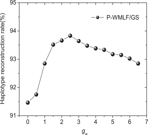
To select a appropriate weighted coefficient g_w, we change g_w from 0 to 6.5, and examine the haplotype reconstruction rate of P-WMLF/GS on the simulated data with n=80, e_s and e_g be randomly selected from 0 to 5%. The experiment result is illustrated by Figure 7. Figure 7 shows that when g_w=2.5, i. e. 1/4 of c, P-WLMF/GS achieves the highest haplotype reconstruction rate. In the following experiments, we set g_w=2.5.

Fig. 7.

The performance of P-WMLF/GS with g_w varying.

When e_s varies from from 3 to 7% and e_g varies from 0 to 7%, we test the three algorithms on both the real haplotype data and the simulated haplotype data with n=100 and m=200. The experiment results are presented in Table 1, in which the experiment results on the real haplotype data are put outside brackets, and the experiment results on the simulated haplotype data are enclosed in brackets. As shown in Table 1, the haplotype reconstruction rate of WMLF/GS and MEC/GI are decreasing with the increasing of e_s and e_g. Since WMLF does not consider the genotype information, its haplotype reconstruction rate is not related with e_g, but is decreasing with the increasing of e_s. Although there are errors planted in the genotype information, the false-genotype alleles are much less than the true-genotype alleles, and the positive impact suppresses the negative impact of the genotype information. For using the genotype information, MEC/GI gets higher haplotype reconstruction rate than WMLF, which is illustrated in Table 1. Anyway, the experiment results on both the real and the simulated haplotype data show consistently that, in the reconstruction rate of haplotypes, WMLF/GS model is about 4% more accurate than MEC/GI model and is about 12% more accurate than WMLF model.

Table 1.

Comparison of the haplotype reconstruction rate of the algorithms with e_s and e_g varying

	Haplotype reconstruction rate (%)
eg	es=3%			es=5%			es=7%
(%)	WMLF/GS	MEC/GI	WMLF	WMLF/GS	MEC/GI	WMLF	WMLF/GS	MEC/GI	WMLF
0	94.6 (94.7)	90.5 (90.7)	80.5 (80.4)	94.2 (94.0)	89.6 (90.5)	79.8 (80.1)	93.6 (93.7)	90.1 (90.3)	80.1 (79.6)
3	94.3 (93.8)	90.2 (89.5)	81.1 (80.3)	92.1 (93.7)	88.3 (89.3)	80.2 (80.0)	92.1 (93.1)	88.6 (88.9)	79.0 (79.5)
5	95.0 (93.8)	89.6 (88.7)	80.0 (80.5)	93.5 (93.2)	89.7 (88.5)	79.3 (80.0)	91.6 (92.6)	87.5 (87.4)	80.0 (79.7)
7	93.9 (93.3)	87.5 (88.7)	79.8 (80.9)	92.9 (93.2)	88.4 (87.9)	79.9 (80.2)	92.8 (93.0)	87.4 (87.3)	80.1 (80.0)

The data not enclosed in brackets are the experiment results on the real haplotype data, and the date enclosed in brackets are the experiment results on the simulated haplotype data. All experiments are repeated 100 times with n=100 and m=200.

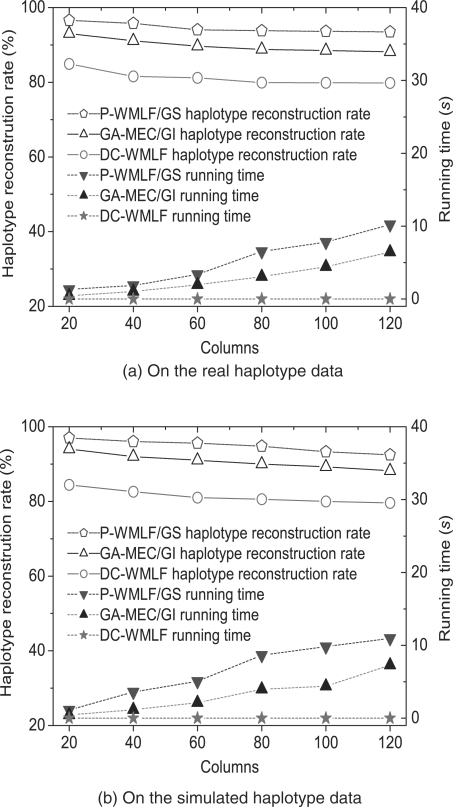
As shown in Figure 8, when e_s=e_g=5%, the experiments on both the real and the simulated haplotype data with n increasing from 20 to 120 also show that P-WMLF/GS is the most accurate algorithm in haplotype reconstruction rate. In Figure 8, the left Y-axis shows the reconstruction rate of haplotypes, and the right Y-axis shows the running time. Figure 8a shows the experiment results on the real haplotype data, and Figure 8b shows the experiment results on the simulated haplotype data. When n increases, the haplotype reconstruction rate of the three algorithms decreases, and their running time increases accordingly. In Figure 8a, when n=20, the haplotype reconstruction rates of P-WMLF/GS, GA-MEC/GI and WMLF are 96.6, 93.0 and 84.9%, respectively; and their running time are 1.3, 0.4 and 0.0007 s. When n increases to 120, their haplotype reconstruction rates decrease to 93.5, 88.1 and 79.8%; and their running time increases to 10.2, 6.5 and 0.008 s. The experiment results in Figure 8b are similar. Although P-WMLF/GS is the slowest among the three algorithms, with the fragment coverage rate fixed, the running time of P-WMLF/GS is a linear function of n, which is very acceptable. The running time of P-WMLF/GS is about 10 s when n=120.

Fig. 8.

The performance comparison of the algorithms when n increases.

5 CONCLUSION

Haplotyping plays an increasingly important role in some regions of genetics such as locating of genes, designing of drugs and forensic applications. The typical computational models of individual haplotyping problem are MFR, MSR, MEC and the variations of MEC. By including the confidence levels a DNA sequencer provides and the genotyping uncertainty, the current article proposes a new computational model WMLF/GS, and proves it to be NP-hard. Based on the fact that the maximum number of fragments covering a SNP site is small (usually no more than 19, Huson et al. (2001)), the current article proposed a parameterized algorithm P-WMLF/GS to solve the WMLF/GS problem. With the fragment maximum length k₁ and the maximum number k₂ of fragments covering a SNP site, the P-WMLF/GS algorithm can solve the WMLF/GS problem in time O(n k₂ 2^{k₂+mlogm+mk₁}) and in space O(m k₁ 2^k₂+nk₂). Extensive experiments show that WMLF/GS has higher haplotype reconstruction rate than other models, and that P-WMLF/GS algorithm is practical.

REFERENCES

- Adkins RM. Comparison of the accuracy of methods of computational haplotype inference using a large empirical dataset. BMC Genet. 2004;5:22. doi: 10.1186/1471-2156-5-22. [DOI] [PMC free article] [PubMed] [Google Scholar]
- Akey J, et al. Haplotypes vs single marker linkage disequilibrium tests: what do we gain? Eur. J. Hum. Genet. 2001;9:291–300. doi: 10.1038/sj.ejhg.5200619. [DOI] [PubMed] [Google Scholar]
- Bonizzoni P, et al. The haplotyping problem: an overview of computational models and solutions. J. Comp. Sci. Technol. 2003;18:675–688. [Google Scholar]
- Carvalho B, et al. Exploration, normalization, and genotype calls of high-density oligonucleotide SNP array data. Biostatistics. 2007;8:485–499. doi: 10.1093/biostatistics/kxl042. [DOI] [PubMed] [Google Scholar]
- Greenberg HJ, et al. Opportunities for combinatorial optimization in computational biology. INFORMS J. Comput. 2004;16:211–231. [Google Scholar]
- Huson DH, et al. Comparing assemblies using fragments and mate-pairs. In. In: Gascuel O, Moret BME, editors. Lecture Notes in Computer Science. Vol. 2149. Berlin/Heidelberg: Springer; 2001. pp. 294–306. Proceedings of the 1st International Workshop on Algorithms in Bioinformatics. [Google Scholar]
- International Human Genome Sequencing Consortium. Initial sequencing and analysis of the human genome. Nature. 2001;409:860–921. doi: 10.1038/35057062. [DOI] [PubMed] [Google Scholar]
- Kang H, et al. Incorporating genotyping uncertainty in haplotype inference for single-nucleotide polymorphisms. Am. J. Hum. Genet. 2004;74:495–510. doi: 10.1086/382284. [DOI] [PMC free article] [PubMed] [Google Scholar]
- Lancia G, et al. SNPs problems, complexity and algorithms. In. In: auf der Heide FM, editor. Lecture Notes in Computer Science. Vol. 2161. Berlin/Heidelberg: Springer; 2001. pp. 182–193. Proceedings of Annual European Symposium on Algorithms (ESA) [Google Scholar]
- Levy S, et al. The diploid genome sequence of an individual human. PLoS Biology. 2007;5:e254–e254. doi: 10.1371/journal.pbio.0050254. [DOI] [PMC free article] [PubMed] [Google Scholar]
- Lippert R, et al. Algorithmic strategies for the single nucleotide polymorphism haplotype assembly problem. Brief. Bioinform. 2002;3:1–9. doi: 10.1093/bib/3.1.23. [DOI] [PubMed] [Google Scholar]
- Myers G. A dataset generator for whole genome shotgun sequencing. In. In: Lengauer T, Schneider R, Bork P, Brutlag DL, Glasgow JI, Mewes HW, Zimmer R, editors. California: AAAI Press; 1999. pp. 202–210. Proceedings of the 7th International Conference on Intelligent Systems for Molecular Biology. [PubMed] [Google Scholar]
- Panconesi A, Sozio M. Fast hare: a fast heuristic for single individual SNP haplotype reconstruction. In. In: Jonassen I, Kim J, editors. Lecture Notes in Computer Science. Vol. 3240. Berlin/Heidelberg: Springer; 2004. pp. 266–277. Proceedings of the 4th International Workshop on Algorithms in Bioinformatics. [Google Scholar]
- The International HapMap Consortium. A haplotype map of the human genome. Nature. 2005;437:1299–1320. doi: 10.1038/nature04226. [DOI] [PMC free article] [PubMed] [Google Scholar]
- Venter JC, et al. The sequence of the human genome. Science. 2001;291:1304–1351. doi: 10.1126/science.1058040. [DOI] [PubMed] [Google Scholar]
- Wang RS, et al. Haplotype reconstruction from SNP fragments by minimum error correction. Bioinformatics. 2005;21:2456–2462. doi: 10.1093/bioinformatics/bti352. [DOI] [PubMed] [Google Scholar]
- Xiao Y, et al. A multi-array multi-SNP genotyping algorithm for affymetrix SNP microarrays. Bioinformatics. 2007;23:1459–1467. doi: 10.1093/bioinformatics/btm131. [DOI] [PubMed] [Google Scholar]
- Xie M, Wang J. An improved (and practical) parameterized algorithm for the individual haplotyping problem mfr with mate-pairs. Algorithmica. 2007 DOI 10.1007/s00453-007-9150-2, http://www.springerlink.com/content/p2202u8wrnr65117/
- Xie M, et al. Research on parameterized algorithms of the individual haplotyping problem. J. Bioinform. Comput. Biol. 2007;5:795–816. doi: 10.1142/s0219720007002710. [DOI] [PubMed] [Google Scholar]
- Zhang XS, et al. Models and algorithms for haplotyping problem. Curr. Bioinform. 2006;1:105–114. [Google Scholar]
- Zhao YY, et al. Haplotype assembly from aligned weighted SNP fragments. Comput. Biol. Chem. 2005;29:281–287. doi: 10.1016/j.compbiolchem.2005.05.001. [DOI] [PubMed] [Google Scholar]
- Zhu WS. Statistical Methods for Haplotype Analysis with Genotyping Errors. Changchun: Northeast Normal University; 2006. Ph. d. thesis. [Google Scholar]