A Genetic Analysis of Mortality in Pigs

Abstract

An analysis of mortality is undertaken in two breeds of pigs: Danish Landrace and Yorkshire. Zero-inflated and standard versions of hierarchical Poisson, binomial, and negative binomial Bayesian models were fitted using Markov chain Monte Carlo (MCMC). The objectives of the study were to investigate whether there is support for genetic variation for mortality and to study the quality of fit and predictive properties of the various models. In both breeds, the model that provided the best fit to the data was the standard binomial hierarchical model. The model that performed best in terms of the ability to predict the distribution of stillbirths was the hierarchical zero-inflated negative binomial model. The best fit of the binomial hierarchical model and of the zero-inflated hierarchical negative binomial model was obtained when genetic variation was included as a parameter. For the hierarchical binomial model, the estimate of the posterior mean of the additive genetic variance (posterior standard deviation in brackets) at the level of the logit of the probability of a stillbirth was 0.173(0.039) in Landrace and 0.202(0.048) in Yorkshire. The implications of these results from a breeding perspective are briefly discussed.

LITTER size has been under selection in the Danish pig breeding program since the early 1990s and this resulted in considerable increase in total number born and also in the proportion of stillborn piglets (Sorensen et al. 2000; Su et al. 2007). A number of studies have reported genetic variation for mortality with heritabilities ranging from 0.03 to 0.12. These studies have either assumed normality of the sampling model for mortality (e.g., van Arendonk et al. 1996) or based inferences on a variety of threshold models (e.g., Roehe and Kalm 2000; Arango et al. 2006), and critical investigations of the quality of fit of the models used were not reported.

Mortality data, regarded as a trait of the mother, show typically a large proportion of zeros (many litters do not have stillborn piglets). Formal genetic analyses of mortality in pigs accounting for this feature of the data are not available in the literature and this article attempts to fill this gap. The focus here is to study the quality of fit and predictive ability of a number of models and to investigate whether they provide statistical evidence for genetic variation for mortality. The statistical genetic analysis involves fitting various hierarchical models involving three discrete distributions: the Poisson, the binomial, and the negative binomial.

The statistical analysis of counts based on discrete parametric distributions has a long and rich history (Johnson and Kotz 1969). In the case of unbounded counts, Poisson regression models are standard, whereas for bounded counts, when the response can be viewed as the number of successes out of a fixed number of trials, regression models based on the binomial distribution are often used (Hall 2000). A restriction of the Poisson model is that it imposes equality of mean and variance. Typically the distribution of counts is overdispersed. In the case of the binomial model the only free parameter is the probability of success, which results in a functional relationship between the mean and the variance. Several possible alternatives have been suggested to obtain more flexible models. For example, the negative binomial distribution has two parameters and allows the mean and variance to be fitted separately (Lawless 1987). An application of the negative binomial model in animal breeding can be found in Tempelman and Gianola (1996, 1999). In the same spirit, a robust alternative to the binomial model is the beta-binomial, which is a mixture of binomials where the unequal probabilities of success vary according to a beta-distribution. In general, hierarchical specifications are needed to explain extra variation that is not accounted for by the sampling model of the data. These involve assigning a distribution to the parameters of the sampling model, directly, as in the case of the negative binomial or beta-binomial models, or indirectly, by embedding these parameters in a linear structure that includes random effects as explanatory variables.

There are situations where overdispersion is partly associated with an incidence of zero counts that is greater than expected under the sampling model, as in the present study. Hurdle models (Mullahy 1986; Winkelmann 2000) and zero-inflated models are two instances of finite mixture models commonly used to account for this characteristic of the data. In the present work the excess of zeros is studied using zero-inflated models that are described in Johnson and Kotz (1969) and extended by Lambert (1992). Ridout et al. (1998) provide a review of various zero-inflated models; recent applications of zero-inflated Poisson models in animal breeding are in Rodriguez-Motta et al. (2007) and in Naya et al. (2008). Zero-inflated models assume that the population consists of two sets of observations. In the first set, which may include zeros, observations are realizations from a discrete sampling process indexed by unknown parameters (this set is often referred to as the imperfect state); observations from the second set consist only of zeros and the parameter of interest is the proportion of these individuals. This set is often referred to as the perfect state. Either or both sets of parameters may depend on covariates.

This article is organized as follows. material and methods describes the data, details of the models, and their Markov chain Monte Carlo (MCMC) implementation. This is followed by a presentation of the results of the analyses and of MCMC-driven explorative tools for model comparison. The article concludes with a discussion.

MATERIALS AND METHODS

Data:

Data were obtained from an existing database of performance records collected from nuclear farms of Danish Landrace and Danish Yorkshire during the period from May 2002 until December 2004. Pedigrees were traced back five generations or more. For Landrace, the data comprised records from 5178 litters and a pedigree file of 8800 individuals. The Yorkshire data consisted of records from 3938 litters and a pedigree file of 7143 individuals. Sows were kept under commercial conditions and all matings took place using artificial insemination. At farrowing, the total number of piglets born per litter and the number of stillborn piglets per litter were recorded.

Models and posterior distributions:

Zero-inflated models assume that the population consists of two subpopulations but the subpopulation membership is not observed. At the first level of the hierarchy of the zero-inflated model, the probability mass function of the response Y_i (number of stillborn piglets in litter i, i = 1, 2, …, n) is given by

(1)

where Y_i has probability mass function f corresponding to the Poisson, binomial, or negative binomial distribution indexed with parameters θ_i, which is assigned probability mass , and the degenerate distribution supported at zero is given probability mass η_i. The standard (non-zero-inflated) version of the models is obtained setting η_i = 0 for all i, in the expressions above.

Standard calculations show that the mean and variance of the zero-inflated random variable Y_i are given by

and

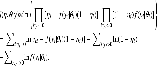
Let , . The loglikelihood takes the form

(2)

For the Poisson model, the probability mass function f in (1), indexed with θ_i = λ_i, is

(3)

with mean and variance .

For the binomial model, with t_i observed, representing the total number born in litter i, the probability mass function is

(4)

where ϕ_i is the probability of a stillborn piglet in litter i. The mean and variance are given by and , respectively. As is well known, with t_i large and ϕ_i small, with their product remaining constant, the binomial distribution converges to the Poisson distribution.

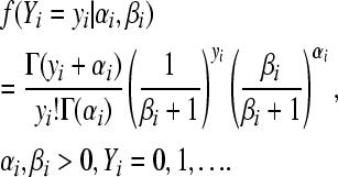
For the negative binomial model, , and

(5)

The mean is and the variance . The negative binomial distribution is the marginal distribution of a Poisson random variable when the rate parameter λ_i has a Gamma distribution with parameters α_i, β_i. In other words, the integral

where

is the probability density function of the Gamma-distribution with parameters α_i, β_i, retrieves (5). The negative binomial model is more flexible than the Poisson and allows for overdispersion. The negative binomial approaches the Poisson with rate parameter α_i/β_i as , with constant.

At the second level of the hierarchy of the model, the following linear structures are assigned. Let the vector logit , where logit is the logit of the probability that the ith observation is a realization from the perfect state. The linear model for logit is

(6)

where b_η is the vector containing effects of herd-year (20 in Yorkshire and 22 in Landrace) and parity (6 in both breeds), u_η is the vector of additive genetic values (7143 in Yorkshire and 8800 in Landrace), and p_η is the vector of permanent environmental effects (3360 in Yorkshire and 4422 in Landrace). The known incidence matrices X, Z, and W associate the relevant vector of location parameters to .

For the Poisson model, define as the vector of the natural logarithm of the Poisson parameter associated with the n litters. As in (6) it is assumed that

(7)

where location parameters and incidence matrices are assigned the same interpretation as in (6). An identical structure was assigned to logit for the binomial model, and to and to for the negative binomial model.

At the third level of the hierarchy the models for the vectors of additive genetic values and permanent environmental effects are assumed to be realizations from the normal distributions

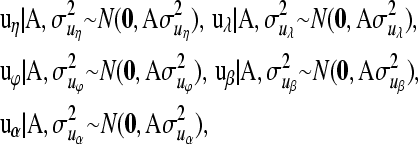where A is the additive genetic relationship matrix, , , , and are additive genetic variance components. Additive genetic values u_η and u_x, x = λ, ϕ, β, α are assumed to be independently distributed. The permanent environmental effects p_z, z = η, λ, ϕ, β, α follow also mutually independent normal distributions , where I is the identity matrix and is the appropriate permanent environmental variance component. The elements of b_z are assumed to follow independent uniform distributions with large absolute values chosen for the bounds.

At the final level of the hierarchy, all variance components where assigned proper uniform distributions with support in the positive real line and large upper bounds.

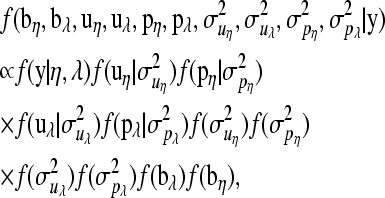
Denote the collection of data by y. For the zero-inflated Poisson model the posterior distribution is

(8)

with

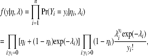and

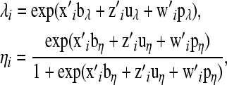where , , and are the ith rows of X, W, and Z, respectively, associated with litter i. The binomial and negative binomial models have the same type of structure as (8).

Model comparison:

The models are compared using the pseudo-log-marginal probability of the data and using a criterion of the model's predictive ability. The pseudo-log-marginal probability of the data is a standard measure of model comparison (Gelfand 1996) and is defined and computed as follows. Consider data vector , where y_i is the ith datum, and y_–i is the vector of data with the ith datum deleted. The conditional predictive distribution has probability mass function

(9)

and can be interpreted as the probability of each data point given the remainder of the data. The actual value of is known as the conditional predictive ordinate (CPO) for the ith observation. The product of CPOs has been proposed as a surrogate for the marginal probability of the data because under mild conditions, the Hammersley–Clifford theorem establishes that the fully conditional distributions uniquely determine the marginal distribution (Besag 1974). The pseudo-log-marginal probability of the data is given by

(10)

and the associated pseudo-Bayes factor (PBF) for comparing two models M₁ and M₂ (Gelfand 1996) is

(11)

A Monte Carlo approximation of the CPO (9) for observation i is given by (Gelfand 1996)

(12)

where N is the number of MCMC draws, M_k is a label for model k, and is the jth draw from the posterior of ϑ_i under model k corresponding to the ith observation.

Each individual CPO, evaluated at Y_i = y_i, yields the probability of observing the datum in question, given the remainder of the observed data and the model. The pseudo-log-marginal probability of the data (10) is a measure of the global fit of a given model. Alternatively, one may be interested in the ability of a given model to predict the proportion of litters showing d stillborn piglets, . One can imagine a situation in which a model generates higher conditional probabilities of each datum than an alternative model, but the latter excels in predicting the proportion of litters showing d stillborn piglets.

Let be the indicator function that takes the value 1 if, for litter i, Y_i = d, and 0 otherwise. Summing over the n litters gives the number of litters in which the number of stillbirths is equal to d. Then the proportion of litters with d stillbirths is a random variable defined as

(13)

The observed proportion of litters with d stillbirths is

(14)

which depends only on the observed data y. A measure of the predictive ability of a model is given by the expected proportion of litters with d stillborn piglets

(15)

which depends on the parameters of the predictive model (it also depends on the total number born in litter i, t_i, in the binomial models).

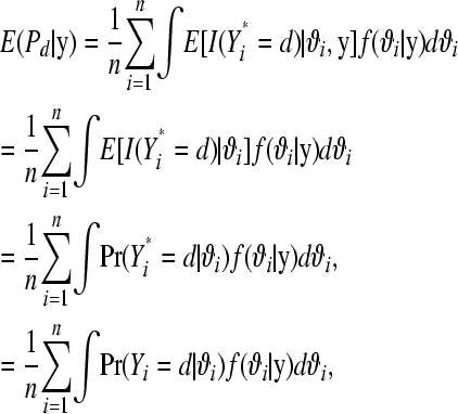
Since parameters are unknown, one can take expectations in (15) conditional on estimates of the η's and θ's or use a posterior predictive analysis (Gelman et al. 1995, 1996) as in subsection MCMC-based analysis. Using the latter approach, uncertainty over the parameters of the model is accounted for by integrating over their posterior distribution. The (posterior) expected proportion of litters with d stillborn piglets is now

(16)

where Y_i* is a random variable with the same probability mass function as Y_i and can be interpreted as a future replication of datum i. The second line follows because by assumption Y_i* is conditionally independent of Y_i given ϑ_i, and the third because . With MCMC, (16) is computed as follows. In the kth MCMC round, k = 1, 2, …, N, for litter i, extract a draw from and compute from (1) setting . Repeat over the n litters and calculate to obtain . Then, averaging over the number of MCMC draws yields a Monte Carlo estimate of .

MCMC implementation:

Posterior distributions of parameters, excluding variance components, are approximated using single-site Metropolis–Hastings updates with random walk proposals. These proposals are uniform distributions centered at the current values, with upper and lower bounds tuned at the values ±0.1σ. For the elements of vector b_x,

for those of vector u_x,

and for p_x,

All variance components are updated using the Gibbs sampler, from scaled inverted χ² distributions.

Convergence of the MCMC chains was studied informally by visual inspection of traceplots of several chosen parameters (not shown). The algorithm showed good mixing properties; we provide Monte Carlo standard errors of estimates of posterior means of chosen parameters to give an idea of the accuracy achieved.

RESULTS

Before reporting results from the Bayesian MCMC analysis based on the various multi-level models described in Models and posterior distributions, results of less formal analyses are shown to illustrate properties of the data and the ability of the various models to capture the most salient features of these properties. The focus here is to compare the quality of fit of nonhierarchical zero-inflated and non-zero-inflated versions within the three models.

Preliminary analysis:

The raw means for total number born for parities 1, 2, 3, 4, and >4 are, respectively, as follows. For Landrace, 13.41, 15.32, 16.13, 16.49, 15.87, and for Yorkshire, 12.33, 14.05, 14.50, 14.55, 14.69. The corresponding raw means for number of stillborn piglets per litter , the raw average squared deviations from the mean across litters, within parities, and the number of litters within parities (S², and n, respectively, in brackets), are, respectively, as follows:

Landrace: 2.35 (5.00;3293), 2.78(6.59; 1110), 3.39(7.64; 492), 3.89(8.87; 181), and 3.95(7.53; 102)

Yorkshire: 1.39(2.98; 2552), 1.45(3.27; 830), 1.94(5.03; 314), 2.53(6.58; 142), and 2.64(7.32; 100).

The averaged squared deviation from the mean is consistently larger than the mean in all parities in both breeds. From these figures, the observed proportion of stillborn piglets in parities 1, 2, 3, 4, and >4 are 0.18, 0.18, 0.21, 0.23, 0.24 in Landrace and 0.11, 0.10, 0.13, 0.17, 0.18 in Yorkshire.

Tables 1 and 2 show observed and predicted proportion of litters with d stillborn piglets (d = 0, 1, 2, 3, 4, > 4) based on all the models for both breeds. The models are as specified in Models and posterior distributions, excluding additive genetic values u and permanent environmental effects p. From a traditional frequentist perspective, these are “fixed effects” models, with parameters herd-years and parity. These models that here are loosely labeled nonhierarchical do not account for the correlated structure of the data due to u and p. The tables report also the loglikelihood, , averaged over the MCMC replicates, as a measure of model fit (e.g., Dempster 1997).

TABLE 1.

Observed (O) (based on Equation 14) and predicted (based on an MCMC implementation of Equation 16) proportion of litters with d stillborn piglets in the Landrace breed, and the average loglikelihood (last row), based on the following models: Poisson (P), zero-inflated Poisson (ZIP); negative binomial (NB), zero-inflated negative binomial (ZINB); binomial (B), zero-inflated binomial (ZIB)

d	O	P	ZIP	NB	ZINB	B	ZIB
0	0.204	0.095	0.199	0.192	0.228	0.091	0.187
1	0.184	0.203	0.177	0.213	0.178	0.198	0.140
2	0.178	0.233	0.206	0.180	0.170	0.235	0.189
3	0.147	0.193	0.172	0.134	0.136	0.200	0.181
4	0.103	0.129	0.115	0.095	0.097	0.134	0.136
>4	0.185	0.147	0.131	0.186	0.191	0.142	0.167
Average loglikelihood		−11350.5	−10745.8	−10629.9	−10612.8	−10877.3	−10553.1

TABLE 2.

Observed (O) (based on Equation 14) and predicted (based on an MCMC implementation of Equation 16) proportion of litters with d stillborn piglets in the Yorkshire breed, and the average loglikelihood (last row), based on the following models: Poisson (P), zero-inflated Poisson (ZIP); negative binomial (NB), zero-inflated negative binomial (ZINB); binomial (B), zero-inflated binomial (ZIB)

d	O	P	ZIP	NB	ZINB	B	ZIB
0	0.384	0.243	0.370	0.379	0.396	0.237	0.373
1	0.239	0.323	0.268	0.252	0.227	0.324	0.194
2	0.160	0.231	0.195	0.153	0.152	0.237	0.189
3	0.092	0.121	0.101	0.089	0.093	0.123	0.129
4	0.051	0.052	0.042	0.051	0.055	0.051	0.068
>4	0.075	0.030	0.024	0.076	0.077	0.028	0.047
Average loglikelihood		−7105.4	−6732.2	−6552.6	−6556.8	−6891.1	−6542.7

The observed number of zeros is severely underpredicted under the nonmixture version of the Poisson and binomial models. The zero-inflated Poisson model provides good predictions for the zero class, but in Landrace underpredicts the proportion of litters with one stillborn piglet and tends to overpredict in parities 2 and 3 in both breeds. The negative binomial model fits the observed data well, with the mixture version showing a slight advantage in Landrace but not in Yorkshire. The binomial model with a single common parameter across litters does not produce good predictions. This changes substantially when extra variation is accounted for by inclusion u and p, as shown in subsection MCMC-based analysis. The results show clearly that within models, in the absence of additive genetic values and permanent environmental effects, the zero-inflated versions provide consistently better fits except for the negative binomial model in Yorkshire; this is also reflected in the comparison between the pairs of loglikelihoods within the three models.

MCMC-based analysis:

Results of the model comparison based on the pseudo-log-marginal probability of the data are shown in Table 3. In both breeds, the data provide very strong support for the hierarchical binomial model. In contrast with the remaining models, the binomial incorporates information on the total number born in each litter. The hierarchical structure of the model at the level of the logit of the probability of a stillborn piglet seems to adequately account for overdispersion without the need for invoking the extra distribution supported at zero.

TABLE 3.

Model comparison for Landrace and Yorkshire based on the sum of the pseudo-log-marginal probability of the data (∑ilnPr(Yi=yi|y−i)) for the following models: Poisson (P), zero-inflated Poisson (ZIP); negative binomial (NB), zero-inflated negative binomial (ZINB); binomial (B), zero-inflated binomial (ZIB)

Breed	P	ZIP	NB	ZINB	B	ZIB
Landrace	−10,775	−10,688	−10,657	−10,630	−10,162	−10,503
Yorkshire	−6,681	−6,572	−6,574	−6,570	−6,358	−6,614

The advantage of the binomial model over the others, in terms of overall fit, is illustrated in more detail in Tables 4 and 5, where the CPOs are averaged for litters with d stillborn piglets . With the exception of the class defined by litters with d = 0 stillborn piglets, the binomial model generates the largest CPOs. The average CPOs of the zero class are a little higher under the zero-inflated binomial model in both breeds.

TABLE 4.

Average CPO (Pr(Yi=d|y−i)) for litters with d stillborn piglets, in Landrace, for the following models: Poisson (P), zero-inflated Poisson (ZIP), negative binomial (NB), zero-inflated negative binomial (ZINB), binomial (B), zero-inflated binomial (ZIB)

d	P	ZIP	NB	ZINB	B	ZIB
0	0.196	0.217	0.213	0.236	0.245	0.262
1	0.235	0.231	0.220	0.195	0.249	0.236
2	0.196	0.194	0.188	0.183	0.203	0.196
3	0.145	0.144	0.143	0.146	0.158	0.156
4	0.103	0.101	0.102	0.107	0.119	0.118
>4	0.048	0.048	0.047	0.049	0.063	0.061

TABLE 5.

Average CPO (Pr(Yi=d|y−i)) for litters with d stillborn piglets, in Yorkshire, for the following models: Poisson (P), zero-inflated Poisson (ZIP), negative binomial (NB), zero-inflated negative binomial (ZINB), binomial (B), zero-inflated binomial (ZIB)

d	P	ZIP	NB	ZINB	B	ZIB
0	0.377	0.432	0.393	0.396	0.405	0.421
1	0.278	0.262	0.262	0.255	0.283	0.255
2	0.162	0.153	0.158	0.160	0.174	0.166
3	0.094	0.089	0.091	0.096	0.110	0.107
4	0.057	0.054	0.054	0.057	0.072	0.068
>4	0.026	0.025	0.023	0.025	0.036	0.029

The figures in Tables 6 and 7 show expected proportion of litters with d stillborn piglets based on the hierarchical models and the observed proportions. The zero-inflated negative binomial hierarchical model has the best predictive ability. There is a remarkable improvement in the quality of predictions of the Poisson and binomial models relative to the nonhierarchical versions.

TABLE 6.

Observed (O) (based on Equation 14) and predicted (based on an MCMC implementation of Equation 16) proportions of litters with d stillborn piglets in Landrace, based on the following models: Poisson (P), zero-inflated Poisson (ZIP); negative binomial (NB), zero-inflated negative binomial (ZINB); binomial (B), zero-inflated binomial (ZIB)

d	O	P	ZIP	NB	ZINB	B	ZIB
0	0.204	0.165	0.175	0.183	0.201	0.166	0.174
1	0.184	0.222	0.219	0.211	0.188	0.216	0.209
2	0.178	0.195	0.192	0.187	0.182	0.191	0.188
3	0.147	0.144	0.142	0.141	0.144	0.145	0.145
4	0.103	0.098	0.098	0.097	0.102	0.102	0.103

TABLE 7.

Observed (O) (based on Equation 14) and predicted (based on an MCMC implementation of Equation 16) proportions of litters with d stillborn piglets in Yorkshire, based on the following models: Poisson (P), zero-inflated Poisson (ZIP); negative binomial (NB), zero-inflated negative binomial (ZINB); binomial (B), zero-inflated binomial (ZIB)

d	O	P	ZIP	NB	ZINB	B	ZIB
0	0.384	0.352	0.386	0.373	0.375	0.349	0.366
1	0.239	0.276	0.262	0.259	0.251	0.273	0.253
2	0.160	0.162	0.154	0.156	0.158	0.164	0.162
3	0.092	0.090	0.085	0.088	0.091	0.093	0.095
4	0.051	0.050	0.047	0.049	0.051	0.052	0.053

In conclusion, the best fitting model (in terms of the pseudo-log-marginal probability of the data) is the hierarchical binomial model, whereas the model that best predicts the proportion of litters showing d stillborn piglets is the zero-inflated negative binomial. These results are a good example of a point made by Rubin (1984). He argued that one may be interested in arriving at more than one inference depending on, for example, whether global fit or prediction of some features of the data capture the relevant scientific objectives of a study.

Statistical evidence for genetic variation for mortality:

The model space is restricted to the globally best fitting model (binomial hierarchical model) and the best predictive model (zero-inflated negative binomial hierarchical model). For the hierarchical binomial model, the MCMC estimates of the means of the posterior distribution of the additive genetic and permanent environmental variances (posterior standard deviations in brackets) are 0.173(0.039) and 0.341(0.034) in Landrace and 0.202(0.048) and 0.566(0.051) in Yorkshire. The sampling uncertainty of the estimates of the posterior means in terms of the Monte Carlo standard errors are 6.0 × 10⁻⁴ and 0.8 × 10⁻⁴ for the additive genetic and permanent environmental variances in Landrace, and 18.54 × 10⁻⁴ and 1.46 × 10⁻⁴ in Yorkshire. Within a given hierarchy, the posterior means indicate that 34 and 26% of the variance is additive genetic in the two breeds.

For the zero-inflated negative binomial hierarchical model, the MCMC estimates of the means of the posterior distribution of the additive genetic and permanent environmental variances (posterior standard deviations in brackets) are, respectively, as follows. In Landrace, at the level of logitη, 0.044(0.019), 1.615(3.643); at the level of lnα, 0.120(0.019), 0.070(0.025); and at the level of lnβ, 0.642(0.313), 2.674(1.654). In Yorkshire, at the level of logitη, 1.136(0.640), 1.114(1.082); at the level of lnα, 0.121(0.036), 0.230(0.052); and at the level of lnβ, 0.627(0.795), 3.550(2.500). There is considerable posterior uncertainty associated with the estimates, with the exception of the additive variance at the level of in both breeds.

The problem is investigated further by computing the pseudo-log-marginal probability of the data under the full model, and under the model where the genetic component of variance is excluded (restricted model). Under the hierarchical binomial model, the pseudo-log-marginal probability of the data in Landrace is – 10, 162 and – 10, 222, under the full and restricted models, respectively. In Yorkshire, these figures are – 6, 358 and – 6, 377. For the zero-inflated negative binomial, in Landrace, these figures are – 10, 657 and – 10, 682, under the full and restricted models, and in Yorkshire, – 6, 574 and – 6, 585. For both models and in both breeds, this analysis supports the existence of genetic variation for mortality.

DISCUSSION

Mortality data in the two breeds of pigs show overdispersion, due to both a high proportion of zeros and heterogeneity induced by covariation among observations. The first source of overdispersion can be accounted for postulating zero-inflated versions of various models for discrete data, and the second invoking a hierarchical structure. In this study we investigated two criteria of the quality of a number of models: global fit and a specific aspect of predictive ability (distribution of stillbirths). Models may not perform equally well under both criteria. Here, a hierarchical zero-inflated negative binomial model was shown to have very good performance on the basis of its ability to predict the distribution of stillborn piglets. On the other hand, the best global fit, measured by the pseudo-log-marginal probability of the data, is obtained with the hierarchical binomial model. The introduction of a hierarchy at the level of the parameters of the model provides flexibility enough to account for both sources of overdispersion, without the need for invoking a mixture as a sampling process. The hierarchical structure provides a natural mechanism to investigate the existence of genetic variation for the trait. Analysis of mortality data based on the binomial hierarchical model and on the zero-inflated negative binomial hierarchical model provided statistical support for the presence of additive genetic variation in both breeds.

From an applied animal breeding perspective, interest may lie in improving survival at weaning rather than focusing on mortality per se. Indeed, Su et al. (2007) showed that a useful strategy to increase number of individuals weaned is to select for number of piglets alive at day 5 after farrowing. This conclusion was based on an approximate analysis invoking multivariate normality as a sampling model for survival rate and number of piglets alive at day 5 after farrowing. This work is less ambitious from a practical perspective and has focused on finding a model that formally accounts for the discrete nature of the data and to study the presence of genetic variation based on such a model. The amount of genetic variation disclosed by the hierarchical binomial model can be exploited to modify the trait by selection and it is of interest to investigate to what extent mortality at birth can be reduced by these means on the basis of this model. The Monte Carlo estimate of the average logit in Landrace is – 1.5265, which is equal to an average probability of a stillborn piglet equal to 18%. The probability of a stillborn piglet among the highest scoring 10% of the individuals on the basis of their additive genetic values is equal to 15%. In Yorkshire, the corresponding figures are 11 and 9%, respectively. The difference between the mean probabilities among selected individuals and the population mean represents expected genetic progress after one cycle of selection. This measure of expected rate of genetic progress is quite consistent with figures for other traits of economic importance.

An extension of the hierarchical binomial model (4) could allow a joint analysis of mortality and litter size, by invoking a model for t, the number of born piglets, rather than doing the analysis of mortality conditioning on it, as was done here. One approach described in Foulley et al. (1987), based on generalized linear models, is to assume that litter size is Poisson distributed and that conditional on litter size, piglet survival, as opposed to mortality, follows a Bernoulli distribution. An alternative is to assume the binomial model (4) for mortality, given litter size t, and to postulate a linear structure for t, along the lines in (6) or (7) with an extra (Gaussian) term to account for residual variation. This would induce normality of the marginal distribution of t, as has been traditionally practiced in analyses of litter size in pigs and mice. Otherwise, t can be assigned a Poisson distribution with parameter λ, whose natural logarithm can be modeled as in (7). In either case, the additive genetic effects at the level of t or of ln λ, and of logit are assumed to follow a multivariate normal distribution. Work along these lines is in progress and results will be reported on a future date.

References

- Arango, J., I. Misztal, S. Tsuruta, M. Culbertson, J. W. Holl et al., 2006. Genetic study of individual preweaning mortality and birth weight in large white piglets using threshold linear models. Livestock Sci. 101 208–218. [Google Scholar]
- Besag, J., 1974. Spatial interaction and the statistical analysis of lattice systems (with discussion). J. R. Statist. Soc. Ser. B 36 192–236. [Google Scholar]
- Dempster, A. P., 1997. The direct use of likelihood for significance testing. Statist. Comput. 7 247–252. [Google Scholar]
- Foulley, J. L., D. Gianola and S. Im, 1987. Genetic evaluation of traits distributed as Poisson-binomial with reference to reproductive characters. Theor. Appl. Genet. 73 870–877. [DOI] [PubMed] [Google Scholar]
- Gelfand, A. E., 1996. Model determination using sampling-based methods, pp. 145–161 in Markov Chain Monte Carlo in Practice, edited by W. R. Gilks, S. Richardson, and D. J. Spiegelhalter. Chapman & Hall, New York.
- Gelman, A., J. B. Carlin, H. S. Stern and D. B. Rubin, 1995. Bayesian Data Analysis. Chapman & Hall, New York.
- Gelman, A., X. L. Meng and H. Stern, 1996. Posterior predictive assessment of model fitness via realized discrepancies (with discussion). Statist. Sinica 6 733–807. [Google Scholar]
- Hall, D. B., 2000. Zero-inflated Poisson and binomial regression with random effects: a case study. Biometrics 56 1030–1039. [DOI] [PubMed] [Google Scholar]
- Johnson, N. L., and S. Kotz, 1969. Distributions in Statistics: Discrete Distributions. Wiley, New York.
- Lambert, D., 1992. Zero-inflated Poisson regression, with an application to defects in manufacturing. Technometrics 34 1–14. [Google Scholar]
- Lawless, J. F., 1987. Negative binomial and mixed Poisson regression. Can. J. Statist. 15 209–225. [Google Scholar]
- Mullahy, J., 1986. Specification and testing of some modified count data models. J. Econometrics 33 341–365. [Google Scholar]
- Naya, H., J. I. Urioste, Y. M. Chang, M. Rodriguez-Motta, R. Kremer et al., 2008. A comparison between Poisson ands zero-inflated Poisson regression models with and application to number of black spots in Corriedale sheep. Genet. Select. Evol. 40 379–394. [DOI] [PMC free article] [PubMed] [Google Scholar]
- Ridout, M. S., C. G. B. Demetrio and J. P. Hinde, 1998. Models for count data with many zeros, pp. 179–192 in Proceedings of the XIX International Biometrics Conference, Cape Town, South Africa.
- Rodriguez-Motta, M., D. Gianola, B. Heringstad, G. J. M. Rosa and Y. M. Chang, 2007. A zero-inflated Poisson model for genetic analysis of number of mastitis cases in Norwegian red cows. J. Dairy Sci. 90 5306–5315. [DOI] [PubMed] [Google Scholar]
- Roehe, R., and E. Kalm, 2000. Estimation of genetic and environmental risk factors associated with pre-weaning mortality in piglets using generalized linear mixed models. Anim. Sci. 70 227–240. [Google Scholar]
- Rubin, D. B., 1984. Bayesianly justifiable and relevant frequency calculations for the applied statistician. Ann. Statist. 12 1151–1172. [Google Scholar]
- Sorensen, D., A. Vernersen and S. Andersen, 2000. Bayesian analysis of response to selection: a case study using litter size in Danish Yorkshire pigs. Genetics 156 283–295. [DOI] [PMC free article] [PubMed] [Google Scholar]
- Su, G., M. S. Lund and D. Sorensen, 2007. Selection for litter size at day five to improve litter size at weaning and piglet survival rate. J. Anim. Sci. 85 1385–1392. [DOI] [PubMed] [Google Scholar]
- Tempelman, R. J., and D. Gianola, 1996. A mixed effects model for overdispersed count data in animal breeding. Biometrics 52 265–279. [Google Scholar]
- Tempelman, R. J., and D. Gianola, 1999. Genetic analysis of fertility in dairy cattle using negative binomial mixed models. J. Dairy Sci. 82 1834–1847. [DOI] [PubMed] [Google Scholar]
- van Arendonk, J. A. M., C. van Rosmeulen, L. L. G. Janss and E. F. Knol, 1996. Estimation of direct and maternal genetic (co)variances for survival within litters of piglet. Livestock Production Sci. 46 163–171. [Google Scholar]
- Winkelmann, R., 2000. Econometric Analysis of Count Data. Springer-Verlag, New York.